Foregrounds for 21cm Observations of Neutral Gas at High Redshift

Abstract

We investigate a number of potential foregrounds for an ambitious goal of future radio telescopes such as the Square Kilometer Array (SKA) and Low Frequency Array (LOFAR): spatial tomography of neutral gas at high redshift in 21cm emission. While the expected temperature fluctuations due to unresolved radio point sources is highly uncertain, we point out that free-free emission from the ionizing halos that reionized the universe should define a minimal bound. This emission is likely to swamp the expected brightness temperature fluctuations, making proposed detections of the angular patchwork of 21cm emission across the sky unlikely to be viable. An alternative approach is to discern the topology of reionization from spectral features due to 21cm emission along a pencil-beam slice. This requires tight control of the frequency-dependence of the beam in order to prevent foreground sources from contributing excessive variance. We also investigate potential contamination by galactic and extragalactic radio recombination lines (RRLs). These are unlikely to be show-stoppers, although little is known about the distribution of RRLs away from the Galactic plane. The mini-halo emission signal is always less than that of the IGM, making mini-halos unlikely to be detectable. If they are seen, it will be only in the very earliest stages of structure formation at high redshift, when the spin temperature of the IGM has not yet decoupled from the CMB.

1 Introduction

We have as yet no direct observational probes of neutral gas beyond the epoch of reionization. One promising technique which has attracted much attention is 21cm tomography of neutral hydrogen (?; ?; ?). 21cm emission and/or absorption from neutral hydrogen at high redshift should exhibit angular fluctuations as well as structure in redshift space. These fluctuations are due to spatial variations in the hydrogen density, ionization fraction, and spin temperature, and may be detectable by future radio telescopes such as the Square Kilometer Array (SKA) and the Low Frequency Array (LOFAR). Although the energy density in 21cm emission is about two orders of magnitude less than the cosmic microwave background (CMB), the extreme smoothness of the CMB both spatially and in frequency space would allow this signal to be teased out. The expected brightness temperature fluctuations on arminute scales is about two orders of magnitude larger than CMB fluctuations. In principle, 21cm tomography would allow us to map out the topology of reionization. This could indirectly constrain the nature of the ionizing sources, telling us whether these sources were faint and numerous or bright and rare. It would thus be an invaluable tool for probing the state of the intergalactic medium during an epoch when traditional probes, such as Ly$\alpha$ absorption, fail (Gunn-Peterson absorption fully saturates at hydrogen neutral fractions $x_{HI}\sim 10^{-4}$).

We present a study of possible foregrounds for these observations. On the arcminute angular scales where the signal is expected to peak, detailed studies of the CMB (involving extrapolation from higher frequencies) tell us that fluctuations in the galactic foreground emission are likely to be relatively unimportant. These galactic foregrounds are fairly well understood and multi-frequency observations should enable us to subtract out both the free-free and synchrotron components (see ? for a detailed discussion). Unresolved extra-galactic radio sources, on the other hand, could give rise to brightness temperature fluctuations which would swamp the expected signal, as discussed by ?. However, this model for source counts was based on surveys with limiting flux densities $\sim 100$mJy at 150 MHz, which were then extrapolated down five orders of magnitude past $\sim 1\mu$Jy (the expected limiting point source sensitivity of SKA). Therefore, as they acknowledge, this estimate of foreground contamination is highly uncertain; a turnover in source counts at lower flux levels could significantly reduce foreground contamination.

We present a minimal estimate of the brightness temperature fluctuations, based on free-free emission from the ionizing sources that reionized the universe (?). We show that brightness temperature fluctuations from these sources exceed the expected signal, making it unlikely that the previously proposed angular 21cm tomography is feasible. We shall show that this estimate is relatively model-independent and depends primarily on the integrated ionizing emissivity.

An inability to detect angular brightness temperature fluctuations need not render 21cm tomography studies powerless. Since the foreground signal is expected to be smooth in frequency space, 21cm spectral features along a pencil-beam slice, corresponding to alternating patches of neutral and ionized hydrogen, could yield invaluable information on the topology of reionization. However, this relies heavily on the lack of foreground spectral contaminants. We investigate two possible contaminants: spectral fluctuations in the foreground due to the frequency-dependent beam, and radio recombination lines from galactic and extragalactic ionized gas. The former can probably be dealt with if the frequency dependence of the beam can be controlled and its side-lobes mapped out. The latter is much more uncertain but is unlikely to be a show-stopper. If, in fact, it does turn out to be important, it will yield the unexpected bonus of new information about the clumping of ionized gas in our galaxy and in the universe as a whole.

In all numerical estimates, we assume a $\Lambda$CDM cosmology where $(\Omega_{m},\Omega_{\Lambda},\Omega_{b}h^{2},h,\sigma_{8h^{-1}})=(0.3,0.7,0.019,0.7,0.9)$.

2 Free-Free Emission from Ionizing Sources as a Foreground

We begin by summarizing the properties of the expected signal; the reader is referred to the literature (?; ?; ?) for details. Consider a patch of IGM, with spin temperature $T_{S}$, which fully fills the beam and has a radial velocity width larger than the bandwidth of the radio telescope. The differential brightness temperature between this patch and the CMB is (?):

$$\delta T_{b}\approx 9.0{\rm mK}h^{-1}\left(\frac{\Omega_{b}h^{2}}{0.02}\right)\left(\frac{1+z}{10}\right)^{1/2}\left(\frac{T_{S}-T_{CMB}}{T_{S}}\right).$$ (1)

Of course, if ionized bubbles exist within this patch then the signal will be diluted by the corresponding filling factor.

Initially, $T_{S}=T_{CMB}$, but over time Ly$\alpha$ photons from the soft UV background emitted by the first stars and quasars will couple the spin temperature of the gas to its kinetic temperature through the Wouthuysen-Field effect. Since initially $T_{K}<T_{CMB}$, neutral hydrogen will be visible for a brief period in absorption until the same Ly$\alpha$ photons also heat the gas through recoil of the scattered Ly$\alpha$ photons and make $T_{S}>T_{CMB}$. At this point the signal is only visible in emission; from equation (1) the brightness temperature is roughly independent of the spin temperature. Hereafter, we shall focus solely on the emission signal.

If linear theory is used to compute expected density fluctuations, the brightness temperature fluctuations peak on arcminute scales and have a rms value of $\langle\delta T_{b}^{2}\rangle^{1/2}\approx 10{\rm mK}$ for a $\Lambda$CDM cosmology (see Fig 1 of ?). To give a sense of the lengthscales involved, a bandwidth $\Delta\nu$ corresponds to a comoving length $L\approx(1+z)cH(z)^{-1}\Delta\nu/\nu=8.6\left(\frac{1+z}{10}\right)^{-3/2}(\Delta\nu/1{\rm MHz})h^{-1}\,{\rm Mpc}$, where $\nu=1.4/(1+z)$Ghz is the observation frequency, and an angular diameter $\Delta\theta$ corresponds to a comoving transverse length $L=\Delta\theta(1+z)/d_{A}(z)\approx 1.9\left(\Delta\theta/1^{\prime}\right)h^{-1}\,{\rm Mpc}$ at z=9.

The contribution of radio-loud AGN and radio galaxies at low flux levels is highly uncertain. We therefore construct a minimal model of the low-frequency radio background from free-free emission by ionizing sources. This background is unavoidable in the sense that a minimal emissivity in ionizing photons is necessary to reionize the universe. We present a brief summary here; refer to ? for details. The free-free luminosity of an ionizing source can be estimated from the fact that the free-free emissivity $\epsilon_{\nu}\propto n_{e}^{2}$ is directly proportional to the recombination rate and thus to the production rate of ionizing photons: $L_{\nu}^{ff}\propto\langle n_{e}^{2}\rangle V\propto\dot{N}^{recomb}\propto(1-f_{esc})\dot{N}_{ion}$. We thus obtain:

$$L_{\nu}^{ff}\approx 1.1\times 10^{27}\left(\frac{\dot{N}_{ion}}{10^{53}{\rm photon\,s^{-1}}}\right)\left(\frac{1-f_{esc}}{0.9}\right){\rm erg\,s^{-1}Hz^{-1}}$$ (2)

where $\dot{N}_{ion}$ is the production rate of ionizing photons, and $f_{esc}$ is the escape fraction of ionizing photons from the host galaxy. For a Salpeter IMF with stars of solar metallicity, $N_{ion}=10^{53}{\rm photons\,s^{-1}}\left({\rm SFR}/1{\rm M_{\odot}yr^{-1}}\right)$. For a given star formation rate (SFR), stars with zero metallicity can be one to two orders of magnitude more effective at producing ionizing photons, since the effective temperature of these stars is higher (?), and the IMF of zero-metallicity stars is often thought to be top-heavy. The escape fraction of ionizing photons is observed to be $f_{esc}\sim 5\%$ in the local universe (?), and thought to decline with redshift (?; ?), although this is highly uncertain (for calculations arriving at the opposite conclusion, see ?). The observed free-free flux is then given by $S_{\rm ff}=L_{\nu}^{\rm ff}(1+z)/4\pi d_{L}^{2}$, or:

$$S_{\rm ff}\approx 1.2\left(\frac{1+z}{10}\right)^{-1}\left(\frac{\dot{N}_{ion}}{10^{53}{\rm photons\,s^{-1}}}\right)\left(\frac{1-f_{esc}}{0.9}\right){\rm nJy}.$$ (3)

Note that the uncertainty in the escape fraction of ionizing photons introduces uncertainties of at most a factor of only a few in the free-free luminosity. Only in the unlikely scenario of virtually all the ionizing photons escaping into the IGM without any photo-electric absorption in the host ISM, would order of magnitude uncertainties creep in as $f_{esc}\rightarrow 1$.

To compute the brightness temperature fluctuations due to these sources, we need to construct a luminosity function. ? followed the star formation model of ?, who assumed that some constant fraction of the gas $f_{*}$ in halos with virial temperatures $T_{vir}>10^{4}$K fragments to form stars, and that each starburst lasts for $\sim 10^{7}$yr. The star formation efficiency parameter $f_{*}$ is tuned for consistency with the observed metallicity of the IGM at z=3, with $f_{*}\sim 1.7-17\%$ corresponding to $Z\sim 10^{-3}-10^{-2}Z_{\odot}$, respectively. With this prescription, $\dot{N}_{ion}\approx 2\times 10^{53}\left(M_{halo}/10^{9}M_{\odot}\right){\rm photons\,s^{-1}}$. Press-Schechter theory can be used to compute the abundance of halos and hence the source counts $dN/dS$. The power spectrum of Poisson fluctuations can then be computed from:

$$C_{l}^{Poisson}=\int_{0}^{S_{c}}dS\frac{dN}{dS}S^{2}$$ (4)

where $S_{c}$ is the minimal flux above which point sources can be identified and removed. The power spectrum due to clustering can be computed from:

$$C_{l}^{clustering}=w_{l}I_{\nu}^{2}$$ (5)

where $w_{l}$ is the Legendre transform of the angular correlation function of sources $w(\theta)$, and $I_{\nu}=\int_{0}^{S_{c}}dS(dN/dS)S$ is the surface brightness of the radio background at frequency $\nu$. The spatial correlation length can be computed from linear theory assuming linear bias; the decrease in the linear growth factor at high-redshift is increased by the number-weighted bias of objects with $T_{vir}>10^{4}$. This results in an angular correlation function $w(\theta)=(\theta/\theta_{o})^{-0.8}$ with a nearly constant angular correlation length $\theta_{o}\sim 2^{\prime}$ independent of redshift for $z>3$ (see Fig. 5 of ?). The rms temperature fluctuations can then be computed from $T_{rms}=\left(l(l+1)C_{l}/4\pi\right)^{1/2}\times c^{2}/2k_{B}\nu^{2}$, where the frequency dependence of the temperature conversion is appropriate in the Rayleigh-Jeans limit. This quadratic frequency dependence implies that the population of free-free emitters only becomes important at low frequencies. Thus, for instance, their existence does not violate any present CMB distortion constraints.

What is the minimal flux $S_{c}$ above which point sources can be identified and removed? The detector noise is: (?):

$$S_{\rm inst}=\frac{2kT_{\rm sys}}{A_{\rm eff}\sqrt{2t\Delta\nu}}\sim 0.3\left(\frac{\Delta\nu}{1\,{\rm MHz}}\right)^{-1/2}\left(\frac{t}{10^{5}\,s}\right)^{-1/2}\,{\rm\mu Jy}$$ (6)

where we have used $A_{\rm eff}/T_{\rm sys}=2\times 10^{8}{\rm cm^{2}K^{-1}}$. On the other hand, the confusion noise is:

$$S_{\rm conf}=\left(C_{l}^{cluster}(S_{c})\theta^{2}\right)^{1/2}\approx 2\left(\frac{S_{c}}{20{\rm nJy}}\right)^{0.3}\left(\frac{\theta}{0.3^{\prime\prime}}\right)^{1.6}{\rm nJy}$$ (7)

Thus, for a 10$\sigma$ detection, the cutoff flux is $S_{c}\sim 20\,{\rm nJy}$. Note that $S_{\rm conf}\propto\left(C_{l}^{cluster}(S_{c})\right)^{1/2}\propto S_{c}^{0.3}$ depends only weakly on the flux cutoff (see Fig. 1 and also Fig. 4 of ?). This is because $C_{l}^{cluster}\propto I_{\nu}^{2}(S_{c})$, and from equation (3) the majority of sources which constitute the free-free background are generally fainter than $\sim 20\,$nJy; removal of rare bright sources has little effect on the mean free-free background $I_{\nu}$. We have assumed unresolved point sources so that $\theta$ is given by the beam resolution; the confusion noise becomes correspondingly larger if the source is extended.

Confusion noise, rather than instrumental noise, is the limiting factor in source identification and removal for free-free sources. The free-free flux is largely frequency-independent. If instrumental noise were the limiting factor, point sources could be identified and removed with higher frequency observations, for which instrumental noise is much lower (for instance, in 10 days a 5$\sigma$ detection of a 16 nJy source at 2 GHz is possible, for a bandwidth $\Delta\nu=1$ GHz). However, since confusion noise is frequency independent, once the confusion limit is reached no further source removal is possible, even with multi-frequency observations.

We compute the Poisson and clustering contributions to the free-free background with the above model. The results are displayed in Figure 1. The 21cm signal is likely to be swamped by Poisson fluctuations at small scales and by fluctuations due to clustering of free-free sources at all scales. This calculation should be compared with that of ?, who use a power law extrapolation of observed number counts to compute the same quantities. Although we arrive at similar conclusions, below we argue that these estimates (in particular the temperature fluctuations due to the clustering component) are significantly more robust.

The results obviously depend on the specifics of the star formation model assumed. Since this is highly uncertain, we highlight here the most robust features of the calculation, which are largely model independent. The number counts in the Poisson signal are dominated by rare bright objects just below the detection threshold $S_{c}$, and can vary widely depending on the shape of the luminosity function at these low flux levels. We therefore disregard this term as it is excessively model dependent. On the other hand, the clustering term, equation (5) is significantly more robust. Our estimate of $\theta_{o}\sim 2^{\prime}$ is likely a minimal estimate of the angular clustering strength since it is dominated by the bias of halos at the threshold virial temperature $T_{vir}\sim 10^{4}$K, which are most abundant. Star formation in lower virial temperature halos, which cannot cool by atomic line cooling, is expected to be extremely inefficient; see e.g. ? for a general review. If, in fact, star formation is more efficient in deeper potential wells (e.g., since feedback processes are less devasting there), the luminosity weighted correlation function will be more heavily weighted towards rare massive halos, which are more highly biased. Thus, the $w_{l}$ term is generally a minimal estimate. The surface brightness term $I_{\nu}^{2}$ is independent of the model for the luminosity function and depends only on the overall normalization of the comoving luminosity density. We can see this from the equation of cosmological radiative transfer (?):

$$I(\nu_{o})=\frac{c}{4\pi}\int_{0}^{\infty}dz\frac{dt}{dz}\frac{\epsilon[\nu_{o}(1+z)]}{(1+z)^{3}}$$ (8)

where $\epsilon(\nu)$ is the comoving emissivity. Since $\epsilon\propto\dot{\Omega}_{*}(1-f_{esc})$ (from equation 3), the radio surface brightness $I(\nu_{o})\propto\Omega_{*}(1-f_{esc})/(1+\bar{z})^{3}$, where $\bar{z}$ is the median redshift at which $\sim 50\%$ of all stars have formed. Thus, a given comoving stellar density $\Omega_{*}$ directly and robustly implies a minimal free-free surface brightness on the sky (the dependence on the star formation history $\dot{\Omega}_{*}(z)$ is weak, since most stars formed at late times). In our calculation we have conservatively included only sources at $z>3$ (which are too faint to be identified and removed) and simply normalized to $\Omega_{*}(z=3)=6\times 10^{-3}\left(\bar{Z}/10^{-2.5}Z_{\odot}\right)\Omega_{b}$, where $\bar{Z}$ is the mean metallicity of the IGM at $z\sim 3$, and we assume a Salpeter IMF where $\sim 1M_{\odot}$ of metals form for every $\sim 100M_{\odot}$ of stars formed. As previously noted, because the majority of sources are significantly fainter than the threshold flux for point source removal $S_{c}$, the mean surface brightness depends only weakly on $S_{c}$ (see Fig. 4 of ?). Since both the estimates for the clustering strength $w_{l}$ and the mean surface brightness $I_{\nu}$ are minimal and robust, we conclude that our estimate for $C_{l}^{cluster}$ constitutes a robust minimal estimate for angular temperature fluctuations on the sky. These fluctuations will swamp the expected brightness temperature fluctuations due to 21cm emission by at least an order of magnitude.

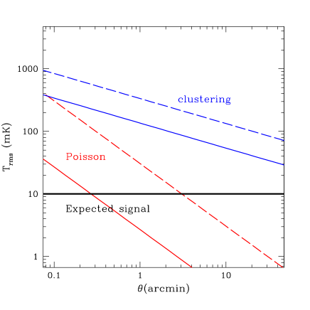
Figure 1: Brightness temperature fluctuations induced by free-free emission from ionizing sources, compared with the expected 21cm signal, at a frequency of 150 MHz (corresponding to an observed redshift of $z=8.3$), and assuming a star formation efficiency corresponding to a Ly$\alpha$ forest metallicity of $Z=10^{-2.5}Z_{\odot}$ at $z=3$. Solid and dashed lines assume point source removal down to 20 nJy and $2\mu$Jy respectively. The 21cm signal is likely to be swamped by fluctuations due to clustering of the free-free sources at all scales. The estimate for the clustering component is fairly robust and model independent (see text). Note that $T_{rms}^{cluster}\propto\Omega_{*}(z=3)\propto Z(z=3)$.

3 Foregrounds for Spectral Measurements

Even if brightness temperature fluctuations due to 21cm emission are not detectable, spectral variation along a pencil-beam might still be detected. This relies on the fact that foreground sources should in general have smooth power-law continuum spectra, and averaging over many sources with different spectral indices and spectral structure will yield a smooth power-low foreground (see ? for simulations of this) which would still allow detection of spectral structure corresponding to alternating regions of neutral and ionized hydrogen. To give an idea of scale, an ionized ’bubble’ created by a source forming stars at a rate $\sim 2{\rm M_{\odot}yr^{-1}}$ for $\sim 10^{7}$yr has a diameter $\sim 1.4[(1+z)/10]^{-1}h^{-1}{\rm Mpc}$ comoving, while a bandwidth $\Delta\nu$ spans a comoving length $L\approx 8.6\left(\frac{1+z}{10}\right)^{-3/2}(\Delta\nu/1{\rm MHz})h^{-1}\,{\rm Mpc}$. Of course, as reionization proceeds the ionized regions expand in size and neutral regions contract. As ? point out, observing with 2 MHz resolution at $\nu_{o}=150$MHz with an error of $\Delta\beta\sim 0.05$ in the measured foreground spectrum spectral slope should allow one to distinguish a signal that is $[(\nu/\nu_{o})^{\Delta\beta}-1]\sim 6\times 10^{-4}$ times smaller than the foreground. Here, we discuss two potential foregrounds for such spectral measurements: beam smearing of foreground sources and radio recombination lines.

The radio telescope does not sample exactly the same patch of sky at all frequencies, since the beam-size and sidelobes are frequency dependent. This would by itself naturally introduce frequency space fluctuations in the measured brightness temperature as additional sources fill the beam, an effect of order:

$$\left(\frac{\Delta T}{T}\right)_{fg} \sim \frac{\Delta\Omega}{\Omega}\sim 2\frac{\Delta\theta}{\theta}\sim 2\frac{\Delta\nu}{\nu}$$

$$\sim 1.4\times 10^{-2}\left(\frac{\Delta\nu}{2{\rm MHz}}\right)\left(\frac{1+z}{10}\right)$$

Since we have seen that the clustering foreground $\langle T^{2}_{fg}\rangle^{1/2}\,\raisebox{-2.58334pt}{$\buildrel>\over{\sim}$}\,10\langle T^{2}_{21cm}\rangle^{1/2}$, the noise in frequency space introduced by beam-size variation will be $\delta T_{fg}\sim{\rm few}\times 0.1\langle T^{2}_{21cm}\rangle^{1/2}$, comparable to temperature fluctuations due to 21cm emission. An exception may be in the very early/late stages of reionization, when the size of ionized/neutral patches is small; the beamsize does not vary signficantly over the small bandwidth $\Delta\nu$ necessary to detect spectral feaures. Otherwise, it would be necessary to develop scaled beams and controlled sidelobes, which are capable of sampling exactly the same patch of sky at all frequencies. Note that frequency calibration of the telescope for pencil beam tomography is considerably more challenging than frequency calibration for detecting an all-sky signal, such as that produced at the tail end of reionization (?). In the case of an all-sky signal, one could simply average the results over many independent patches of sky, as well as perform a differencing experiment off the moon, which blocks emission behind it (?).

Another possible source of structure in frequency space is the signal from radio recombination lines (RRLs). These lines have been observed both in emission and absorption at a wide range of frequencies, although generally only against bright sources in the Galactic plane (see ? for a comprehensive review). The frequencies of the hydrogen lines are:

$$\nu\approx 153\Delta n\left(\frac{n}{350}\right)^{-3}{\rm MHz}.$$ (10)

The important question is whether RRLs will provide a significant source of contamination on lines of sight outside the Galactic plane. There have been few RRL line searches away from bright sources outside the Galactic plane, and in any case surveys for radio recombination lines generally have low-frequency detection limits above the strength of the 21cm features we seek. We can place a useful limit using the fact that the observed brightness of both RRL and H$\alpha$ emission depends on the emission measure $EM=\int dsn_{e}^{2}$, and that optical surveys for H$\alpha$ have much lower limiting sensitivities. Fabry-Perot surveys have detected H$\alpha$ emission from every Galactic latitude, with minimal values $0.25-0.8$ Rayleighs toward the Galactic pole (?). The emission measure corresponding to an observed H$\alpha$ intensity $I_{\alpha}$ (in Rayleighs) is: $EM(H\alpha)=2.75T_{4}^{0.9}I_{\alpha}{\rm cm^{-6}pc}$. Based on the width of the H$\alpha$ line, ? estimates $T\sim 8000$K. Given the density, temperature and size of a region, as well as an estimate of the linewidth and a frequency to observe at, one can also calculate the recombination line optical depth (?):

$$\tau_{L}=\frac{518EM}{\nu\Delta V_{L}T_{e}^{5/2}}b_{n}\left[1-20.8\frac{T_{e}}{\nu}\frac{d\ln b_{n}}{dn}\right],$$

where $EM$ is the emission measure in cm${}^{\textrm{-}6}$pc defined by $n_{e}^{2\ }l$, $\nu$ is the line center frequency, $V_{L}$ is the line width in km/s, $T_{e}$ is the electron temperature, and $b_{n}$ is the departure coefficient, which takes into account departures from local thermodynamic equilibrium (LTE). For LTE, $b_{n}\equiv 1$. For an unresolved line, the velocity width is simply: $\Delta V_{L}=c(\Delta\nu/\nu)$, where $\Delta\nu$ is the observational bandwidth. Assuming $I_{\alpha}=0.25R$ (which corresponds to $EM=0.5{\rm cm^{-6}pc}$) and $T_{L}=\tau_{L}T_{e}$, we can employ the optical depth calculation to estimate the hydrogen RRL temperature:

$$T_{L}=1.3\times 10^{-6}\left(\frac{T_{e}}{8000K}\right)^{-3/2}\left(\frac{EM}{0.5{\rm cm^{-6}pc}}\right)\left(\frac{\Delta\nu}{1{\rm MHz}}\right)^{-1}\,{\rm K}$$ (11)

which is negligible. Note, however, that this estimate assumes thermodynamic equilibrium. Particularly for lower frequency lines, stimulated emission may become important.

Carbon radio recombination lines are another possible source of contamination. They have been detected in the frequency range 34-325 MHz toward Cass A in the Galactic plane (?), and also in a 327 MHz survey centered at $b=14^{\circ}$ (?). Optical depths are generally $\tau\sim 10^{-3}$ and they are thought to arise in dense, cold ($T_{e}\sim 20-200$K), partially ionized regions where non-LTE effects are important. Carbon RRL emission is generally confined to $b<3^{\circ}$ and their intensity out of the plane is probably small (?).

Detections of radio recombination lines from extragalactic sources have generally been confined to bright starburst galaxies and the intensity appears to be correlated with the star formation rate (?). They are unlikely to be significant contaminants. One can show that for reasonable assumptions about the excitation parameter only nearby sources ($D\leq 10$Mpc) will be detectable in RRL emission if spontaneous emission is responsible (?). It was thought that stimulated emission could allow observation of much more distant sources (?), but that has not turned out to be the case.

Extragalactic RRLs could be a foreground in the search for 21cm absorption against radio-loud sources at high redshift (?; ?). Since high-redshift objects are in general much denser $n_{e}^{2}\propto(1+z)^{6}$, their emission measures are much higher. Consider an isothermal disk at temperature $T_{gas}$ embedded in a halo with virial temperature $T_{vir}$. One can solve for the density profile of such a disk, $n\propto{\rm exp}(-r/R_{d}){\rm sech^{2}}(z/z_{o})$ (?; see also ?), and the emission measure of the disk will be $EM(r)\approx\int dzn^{2}(r,z)$. For a disk seen face-on, the emission measure becomes a function of the radial distance $r$ from the center:

$$EM(r)\approx 2\times 10^{9}\left(\frac{f_{\rm d}}{0.5}\right)^{3}\left(\frac{T_{\rm gas}}{10^{4}\,{\rm K}}\right)^{-1}\left(\frac{T_{\rm vir}}{5\times 10^{4}\,{\rm K}}\right)^{3/2}$$

$$\times\left(\frac{\lambda}{0.05}\right)^{-6}\left(\frac{1+z}{10}\right)^{9/2}{\rm exp}\left(-\frac{2r}{R_{\rm d}}\right)\ {\rm cm^{-6}pc}$$ (12)

where $f_{d}=(M_{disk}/M_{halo})/(\Omega_{b}/\Omega_{o})$ is the fraction of baryons in the disk, $\lambda$ is the spin parameter and $R_{d}\approx\lambda r_{vir}/\sqrt{2}$. The optical depth at line center for a $\Delta n=1$ RRL will be:

$$\tau_{L}=2\times 10^{-2}\left(\frac{T_{e}}{10^{4}K}\right)^{-5/2}\left(\frac{EM}{10^{8}{\rm cm^{-6}pc}}\right)\left(\frac{\Delta\nu}{1{\rm MHz}}\right)^{-1},$$ (13)

assuming local thermodynamic equilibrium and that the line is unresolved. This could be considerably enhanced if stimulated emission and/or non-LTE effects become important (which is likely since one is looking along the line of sight to a radio-bright source). This optical depth is comparable to the central optical depths due to 21cm absorption by the IGM (?) or mini-halos/mini-disks (?), which are of order $\tau\sim 10^{-2}$. If one uses Press-Schechter theory to calculate abundances of halos with $T_{vir}>10^{4}$K, a random line of sight would intersect $\sim{\rm few}\times 0.1$ disks per redshift interval, for the redshifts of interest (?). Even a single disk along the line of sight would introduce a plethora of RRL features in emission and/or absorption. This would make the task of picking out the spectral features due to 21cm absorption much more difficult. On the other hand, such observations would also be an invaluable probe of gas clumping at high redshift. However, this is a rather speculative scenario, and we shall not comment on it further.

In general, radio recombination lines are unlikely to be significant contaminants. If they are, they will have to be removed with observations of higher spectral resolution (using the fact that they occur at known frequency intervals for identication and removal). In many ways their detection could be an unexpected bonus, as RRLs have the potential to teach us a great deal about the clumping of ionized gas both within our Galaxy and in the universe as a whole.

4 Detection of Mini-Halos

Recently, it has been proposed that mini-halos with $T<10^{4}$K, which are not collisionally ionized but which have gas densities sufficiently high to collisionally couple the spin temperature to the kinetic temperature, may be detectable in emission (?; ?). For $T_{S}\gg T_{CMB}$, the flux is independent of the spin temperature and depends only on the HI mass. Although the signal from an individual mini-halo is very faint, the combined signal from many mini-halos within a sufficiently large comoving volume may be detectable. We point out that because $S_{\nu}\propto M_{HI}$, the flux from mini-halos will always be swamped by the flux from the neutral IGM, as the HI mass in the IGM is larger. The ratio of fluxes is given by the relative fraction of HI in collapsed halos with $T_{vir}<10^{4}$K:

$$\frac{S_{\nu}^{halos}}{S_{\nu}^{IGM}}\approx\frac{\Omega_{HI,halos}}{\Omega_{HI}}\approx\frac{1}{\rho_{m}}\int_{M_{low}}^{M_{high}}dM\frac{dN}{dM}{M}$$ (14)

where $dN/dM$ is the halo abundance given by Press-Schechter theory, $M_{high}=10^{8}[(1+z)/10]^{-3/2}{\rm M_{\odot}}$ is the mass of halos with $T_{vir}=10^{4}$K, and $M_{low}$ is the baryonic Jeans mass below which gas cannot accrete onto halos. If there is no heating of the IGM, $M_{low}$ is given by the cosmological Jeans mass $M_{J}=8\times 10^{3}[(1+z)/10]^{3/2}{\rm M_{\odot}}$, where the temperature of the IGM $T_{IGM}=1.7[(1+z)/10]^{2}$K is simply set by the amount of adiabatic cooling since decoupling from the CMB. In reality it is likely that the gas will be heated up to higher temperatures by soft X-ray and Ly$\alpha$ photon recoil heating from the first sources of light, as well as by free-free emission from collapsing structures (?). This will suppress the accretion of gas onto the smallest mini-halos.

We plot the ratio of fluxes from equation (14) in Fig (2). Even if heating is negligible, this ratio is at most a ${\rm few}\times 0.1$. This may be amplified in high density peaks by a factor of no more than a few due to clustering bias (?). Thus, the flux from mini-halos only dominate in two limits: (i) in reionized regions, for self-shielded mini-halos which have not yet been photo-evaporated, and (ii) very early in the structure formation process, when the background radiation field is low and the spin temperature of the IGM is still coupled to that of the CMB. The former case is unlikely to be detectable as the mini-halos contribute a small signal superimposed on the much larger fluctuating signal of alternating neutral and ionized regions of the IGM. The latter may be detectable provided the mini-halos indeed remain neutral and do not form stars via ${\rm H_{2}}$ cooling: even a single star in a halo is capable of photo-ionizing and photo-evaporating much of the gas.

Figure 2: Relative 21cm flux from mini-halos compared to IGM in a neutral patch which fills the beam, assuming $T_{S}\gg T_{CMB}$ for both. Since $S_{\nu}^{halos}/S_{\nu}^{IGM}=\Omega_{halos}/\Omega_{b}$, the 21cm emission from the IGM will always be greater except in the earliest stages of structure formation when the spin temperature of the IGM is still coupled to that of the CMB. The relative mass fraction (and hence 21cm flux) in mini-halos decreases still further if the IGM is heated to ’warm’ temperatures (e.g. $T_{IGM}\sim{\rm 200K,2000K}$ as shown here) by soft X-rays or atomic recoil from Ly$\alpha$ photon scattering, which increases the baryonic Jeans mass and suppresses accretion onto mini-halos.

It is worth checking if this is possible. From ? (see their Fig. 6), the level of background UV flux capable of photo-dissociating ${\rm H_{2}}$ in mini-halos and preventing star formation is:

$$J_{diss}\sim 10^{-3}-10^{-2}J_{21}$$

in the redshift range z=10-20 where $J_{21}$ (in units of $10^{-21}{\rm ergs^{-1}cm^{-2}Hz^{-1}sr^{-1}}$) is the UV flux in the Lyman-Werner bands $11.2-13.6$eV. On the other hand, the critical thermalization flux of Ly$\alpha$ photons (which consists of redshifted photons from the Lyman-Werner bands) required to decouple the spin temperature of the IGM from the CMB and drive $T_{S}\rightarrow T_{K}$ is (?):

$$J_{therm}\approx 0.9J_{21}\left(\frac{1+z}{10}\right).$$

Since $J_{diss}\ll J_{therm}$, there certainly exists a period in the history of the IGM where gas in mini-halos cannot cool to form stars, but the IGM does not emit in 21cm radiation. In this case, the halos would give rise to a period in which 21cm is detectable in emission before it is seen in absorption when $T_{S,IGM}<T_{CMB}$. 21 cm radiation would once again be detectable in emission due to heating when $T_{S,IGM}\gg T_{CMB}$. The duration of each of these epochs can be used to time the rise of the radiation field. Of course, this is all assuming that the noise from foregrounds previously discussed can be overcome for the smaller signal levels expected from mini-halos. Note that a period of early reionization would wipe out the mini-halo population by raising the baryonic Jeans mass (?). Also, early star formation would provide trace metal contamination, and if $Z\,\raisebox{-2.58334pt}{$\buildrel>\over{\sim}$}\,10^{-3}Z_{\odot}$ (?), the gas in mini-halos would be able to cool via metal line cooling and form stars. If the mini-halo signal is detectable in spectral pencil-beam measurements, it is preferable to have as small a bandwidth as possible ($\sim 0.1$MHz) to maximize intensity fluctations due to the varying number of halos within a bandwidth along the line of sight.

5 Conclusions

We have considered a number of foregrounds for 21cm emission studies. We perform a robust minimal estimate of temperature fluctuations across the sky due to free-free emission by ionizing sources assuming only: (i) a number-weighted clustering bias with a cutoff for halos with $T_{vir}<10^{4}$K, (ii) a star formation history normalized to the metallicity of the z=3 Ly$\alpha$ forest, and (iii) an escape fraction of ionizing photons into the IGM of no more than $\sim{\rm few}\times 0.1$. We conclude that the clustering component of temperature fluctuations will swamp the expected angular brightness temperature fluctations due to 21cm emission during the cosmological Dark Ages by at least an order of magnitude. Performing 21cm tomography by detecting spectral features along a single line of sight requires developing scaled beams which sample exactly the same patch of sky at all frequencies. Otherwise, excess variance in foreground sampling due to the frequency dependence of the beam will swamp the signal. We also discuss radio recombination lines as possible contaminants. It is unlikely that this will be a problem for surveys outside of the Galactic plane, although this is still fairly uncertain.

Detection of a 21cm spectral signature in absorption against a high-redshift radio loud source (?; ?) will not suffer from the foregrounds discussed here, except for the rather speculative possibility that intervening high-redshift disks could give rise to a plethora of obscuring radio recombination lines. Of course, this ’foreground’ would itself be a marvellous window on the high-redshift universe! The main difficulty of absorption studies, of course, is whether such bright radio sources exist at early times, when structure formation is in its infancy.

References

- [Barkana & Loeb ¡2001¿] Barkana, R., & Loeb, A., 2001, Phys. Rep., 349, 125
- [Bromm et al ¡2001¿] Bromm, V., Ferrara, A., Coppi, P.S., & Larson, R.B. 2001, MNRAS, 328, 969
- [Carilli, Gnedin & Owen ¡2002¿] Carilli, C.L., Gnedin, N.Y., & Owen, F., 2002, ApJ, 577, 22
- [Cen ¡2002¿] Cen, R., 2002, ApJ, submitted, astro-ph/0210473
- [Di Matteo et al ¡2002¿] Di Matteo, T., Perna, R., Abel, T., & Rees, M.J., 2002, ApJ, 564, 576
- [Fujita et al ¡2002¿] Fujita, A., Martin, C.L., Mac Low, M.-M., & Abel, T., ApJ, submitted, astro-ph/0208278
- [Furlanetto & Loeb ¡2002¿] Furlanetto, S.R., & Loeb, A., 2002, ApJ, 571, 1
- [Gordon & Sorochenko ¡2002¿] Gordon, M.A., & Sorochenko, R.L., 2002, Radio Recombination Lines: Their Physics and Astronomical Applications, Kluwer, Dordrecht
- [Gnedin & Ostriker ¡1997¿] Gnedin, N.Y., & Ostriker, J.P., 1997, ApJ, 486, 581
- [Haiman & Loeb ¡1997¿] Haiman, Z., & Loeb, A., 1997, ApJ, 483, 21
- [Haiman, Abel & Rees ¡2000¿] Haiman, Z., Abel, T., & Rees, M.J., 2000, ApJ, 534, 11
- [Iliev et al ¡2002a¿] Iliev, I.T., Shapiro, P.R., Ferrara, A., & Martel, H., 2002a, ApJ, 572, L123
- [Iliev et al ¡2002b¿] Iliev, I.T., Scannapieco, E., Martel, H., & Shapiro, P.R., 2002b, MNRAS, submitted, astro-ph/0209216
- [Leitherer et al ¡1995¿] Leitherer, C., et al 1995, ApJ, 454, L19
- [Madau, Meiskin & Rees ¡1997¿] Madau, P., Meiskin A., & Rees, M.J., 1997, ApJ, 475, 429
- [Oh ¡1999¿] Oh, S.P., 1999, ApJ, 527, 16
- [Oh & Haiman ¡2002¿] Oh, S.P, & Haiman, Z., 2002, ApJ, 569, 558
- [Payne et al ¡1989¿] Payne, H.E., Anantharamaiah, K.R., & Erickson, W.C., 1989, ApJ, 341, 690
- [Peebles ¡1993¿] Peebles, P.J.E., 1993, Principles of Physical Cosmology, Princeton University Press, Princeton
- [Phookun et al ¡1998¿] Phookun, B., Anantharamaiah, K.R., & Goss W.M., 1998, MNRAS, 295, 156
- [Reynolds ¡1990¿] Reynolds, R.J., 1990, in S. Bowyet & C. Leinert (eds), Galactic and Extragalactic Background Radiation, Proc. IAU Symp. No. 139, Kluwer, Dordrecht, p. 157
- [Ricotti & Shull ¡2000¿] Ricotti, M., & Shull, J.M., 2000, ApJ, 542, 548
- [Rohlfs & Wilson ¡1996¿] Rohlfs, K., & Wilson, T.L., 1996, Tools of Radio Astronomy (Berlin:Springer)
- [Roshi et al ¡2002¿] Roshi, D.A., Kantharia, N.G., & Anantharamaiah, K.R., 2002, A&A, 391, 1079
- [Scott & Rees ¡1990¿] Scott, D., & Rees, M.J., 1990, MNRAS, 247, 510
- [Shaver ¡1975¿] Shaver, P.A., 1975, A&A, 43, 465
- [Shaver ¡1978¿] Shaver, P.A., 1978, A&A, 68, 97
- [Shaver et al ¡1999¿] Shaver, P.A., Windhorst, R.A., Madau, P., & de Bruyn, A.G., 1999, A&A, 345, 380
- [Tozzi et al ¡2000¿] Tozzi, P., Madau, P., Meiskin, A., & Rees, M.J., 2000, ApJ, 528, 597
- [Tumlinson & Shull ¡2000¿] Tumlinson, J., & Shull, M.J. 2000, ApJ, 528, L65
- [Wood & Loeb ¡2000¿] Wood, K., & Loeb, A., 2000, ApJ, 545, 86