What can we learn about extragalactic radio jets from X-ray data?

D. E. Harris

Abstract

We review the current status of resolved X-ray emission associated with extragalactic radio jets and hotspots. The primary question for any particular jet is to decide if the X-rays come from the synchrotron process or from inverse Compton scattering. There is considerable evidence supporting synchrotron emission for knots in the jets of FRI galaxies. For FRII terminal hotspots detected in the X-ray band, synchrotron self-Compton emission continues to provide viable models with one possible exception (so far). Inverse Compton scattering on photons of the cosmic microwave background is indicated for a few powerful jets, and is expected to be an important contributor if not the dominating mechanism for higher redshift objects. The application of a model generally yields physical parameters and in many cases, these include the Doppler boosting factor.

SAO, 60 Garden St., Cambridge, MA 02138, USA; harris@cfa.harvard.edu

1. Introduction

The study of relativistic jets via X-ray emission provides certain key advantages unobtainable at lower frequencies. If the X-rays come from synchrotron emission, then we are dealing with Lorentz energies $\gamma\approx 10^{7}$ . This fact leads to two important features: $E^{2}$ halflives are very short which means that observed emission regions correspond to sites of injection or acceleration of particles, and that variability timescales are of order a year or less. For the most part, X-ray variability has been limited to unresolved cores; whereas now we can observe variability for knots which are well separated from the nucleus (Harris et al. 2003).

If the X-ray emission arises from the inverse Compton (IC) process, then we are dealing with electrons for which $\gamma\leq 1000$ and thus we can obtain amplitudes of the electron spectra at energies not available to ground based radio observations.

For the case of synchrotron self-Compton emission (SSC), we are able to estimate the average magnetic field strength and for the case of equipartition fields, constrain the filling factor and the contributions to the total particle energy density from low energy electrons and from protons.

In this overview which is limited to jet knots and hotspots clearly distinct from emission associated with the nucleus, we discuss the emission processes and summarize what we have learned so far. We end with a discussion of some of the current problems and goals. We concentrate on aspects for which new information has become available subsequent to a previous short review prepared for a meeting in 2000 August (Harris 2002) and discussions on the enhancement of IC scattering on the cosmic microwave background (CMB) experienced by relativistic jets (Celotti, Ghisellini, & Chiaberge. 2001; Tavechhio et al. 2000; Harris & Krawczynski 2002).

We maintain a website (http://hea-www.harvard.edu/XJET/) which currently lists 37 radio galaxies and quasars with known X-ray emission from jets or hotspots. Before the launch of the Chandra X-ray Observatory, this table had only 7 entries: 3C273, Cen A, M87, Cyg A, Pic A, 3C120, and 3C390.3.

2. X-ray Emission Processes and what they reveal

For any given feature, it is necessary to identify the emission process before we can estimate physical parameters. For knots and hotspots there is no longer any serious consideration given to thermal emission, although X-ray emission from hot gas may be closely associated with jets in some cases. The main problem is to decide between synchrotron and IC emissions (the latter comes of course in many different flavors depending on the nature of the target photons). Every synchrotron source must also produce IC emission from at least the CMB and the synchrotron photons; our question is, which process dominates the X-ray emission.

2.1. Synchrotron Self-Compton Emission

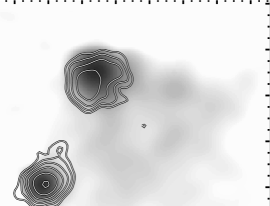
SSC emission models have been successfully applied to several terminal hotspots of FRII radio galaxies and the resulting magnetic field strengths are close to equipartition for filling factors close to 1 and little or no contribution to the particle energy density from protons (Harris 2002). Hardcastle et al. (2002) have recently added to the small number of FRII hotspots with sufficiently large photon energy densities to provide detectable SSC X-rays. In figure 1 we show one of their sources, the double hotspot in the quasar 3C 351. This is not a typical SSC hotspot, nor is it a typical FRII radio structure since the hotspot on the other side of the source is very weak. It is one of the few where the X-ray emission is substantially greater than predicted by SSC with equipartition fields. Here, and in the western hotspot of Pic A, Doppler boosting, a significant departure from equipartition, and/or a substantial contribution from synchrotron emission are possible explanations for the excess emission.

Refer to caption — Figure 1.: The double hotspot system in 3C351. The greyscale shows an 8GHz VLA map with a beamsize of 0.86^′′, comparable to the Chandra resolution. The contours are from the Chandra X-ray image smoothed with a Gaussian of FWHM= $0.5^{\prime\prime}$ . Contour levels increase by factors of two. Note that the northern hotspot is well resolved in the X-rays, and that there is a significant mismatch between the X-ray and radio morphologies. For most SSC hotspots, the X-ray morphology closely mimics the radio structure.

2.2. IC/CMB

The notion that kpc scale jets of FRII sources are still moving with significant bulk relativistic velocity was argued by Bridle (1996) and others. Celotti et al. (2001) and Tavecchio et al. (2000) suggested that in the jet frame, the photon energy density, $u(\nu)$ , of the CMB would be augmented by $\Gamma^{2}$ ( $\Gamma$ is the jet’s Lorentz factor), and this could shift the primary energy loss mechanism from the normally dominate synchrotron channel to the IC channel, thus increasing the ratio of the IC to synchrotron luminosities. These authors successfully applied this idea to the jet of PKS0637 and derived $\Gamma\approx~{}10$ for equipartition fields. However, when the model is applied to low redshift FRI radio galaxy jets, it fails since extremely large values of $\Gamma$ , coupled with unreasonably small angles of the jet to the line of sight, are required (Harris & Krawczynski 2002).

Once the redshift becomes significant, the (1+z)⁴ term in the energy density of the CMB becomes increasingly important, and for such sources, the ’heavy lifting’ to increase u( $\nu$ ) comes from the redshift rather than the $\Gamma^{2}$ term (see e.g. Siemiginowska et al. 2002).

2.3. Synchrotron Emission

Synchrotron X-ray emission is normally modeled by extending the powerlaw distribution of electron energy (with or without breaks) to Lorentz factors, $\gamma$ , of $10^{7}$ to $10^{8}$ . This sort of model can be applied to most or all X-ray knots in the jets of FRI sources and does not require excessive amounts of energy. It is true however that the E² lifetimes are short, and hence observed X-ray emission must demarcate injection/acceleration regions.

When constructing synchrotron (or IC) models, we often obtain estimates of the beaming parameters as a by product. In the case of the knot HST-1 in the M87 jet, we were able to demonstrate that the variability characteristics were consistent with a synchrotron model, but not with IC emission (Harris et al. 2003). Moreover, by solving for synchrotron parameters for a range of Doppler factors $\delta$ , it was found that the observed decay rates in the lightcurves (harder X-rays decay faster than softer X-rays) were consistent with synchrotron losses in a field of order 1 mG with $\delta\approx~{}3$ .

To relate the decay of the lightcurve to a synchrotron loss model, we start with the normal synchrotron equations (Pacholczyk 1970) and make the simplifying assumption that if the emission in a small band drops by a certain amount, then there will be a proportionally smaller number of electrons after the drop. Although this approach assumes that the magnetic field strength remains constant, it demonstrates the method of obtaining parameters.

The electron spectrum is the usual power law.

N(E)~{}=~{}k_{e}~{}E^{-p}

(1)

Synchrotron losses go as $E^{2}$ ( $c_{1}$ & $c_{2}$ are constants):

\frac{dE}{dt}~{}=~{}c_{2}~{}B^{2}~{}E^{2}~{}erg~{}s^{-1}

(2)

Consider a segment of the electron energy distribution responsible for a given observed X-ray band between $\nu_{1}$ and $\nu_{2}$ . Let $h\equiv\frac{\nu_{2}}{\nu_{1}}$ . The number of electrons entering the band (per sec) at $E_{2}$ will be $N(E_{2})\times~{}\frac{dE_{2}}{dt}$ and the number leaving at $E_{1}$ will be $N(E_{1})\times~{}\frac{dE_{1}}{dt}$ .

The net change will be

\Delta~{}N=N(E_{1})~{}\frac{dE_{1}}{dt}~{}[h^{1-\frac{p}{2}}~{}-~{}1]~{}s^{-1}

(3)

and for a drop in flux, f(t), over some given time, $t^{\prime}=t^{\prime}_{2}~{}-~{}t^{\prime}_{1}$ (primes denote the jet frame):

\frac{f(t^{\prime}_{2})}{f(t^{\prime}_{1})}=\frac{\int~{}N(E,t^{\prime}_{1})~{}+~{}t^{\prime}\times\Delta~{}N}{\int~{}N(E,t^{\prime}_{1})}

(4)

With $t^{\prime}=\delta~{}t_{o}$ and $E^{\prime}=\sqrt{\frac{\nu}{\delta~{}c_{1}~{}B}}$ , we find:

\delta~{}B^{3}~{}=~{}\frac{c_{1}}{\nu_{1}}~{}\frac{1}{t_{o}^{2}~{}c_{2}^{2}}~{}\left[1~{}-~{}\frac{f(t_{2})}{f(t_{1})}\right]^{2}~{}~{}\frac{1}{(p-1)^{2}}~{}\left[\frac{h^{(1-p)/2}-1}{h^{(1-p/2)}-1}\right]^{2}

(5)

All the terms on the far right depend only on the spectral index and the bandwidth. In the center we have the ratio of fluxes at two times, and the time between intensity observations is given by t_o. Thus on the right are observables, providing a measure of $\delta~{}B^{3}$ which can be compared with this product from trial $\delta$ s and resulting equipartition fields (see Harris et al. 2003 for the relevant table). For the 3 energy bands used in the M87 analysis of HST-1, we find $\delta=3.3\pm 1$ (slightly different values are obtained if $\alpha\neq 1.0$ )

This ’modest beaming’ model is consistent with beaming parameters deduced from proper motions of substructures in the same knot at optical wavelengths (Biretta, Sparks, & Macchetto 1999).

3. Problems

3.1. High frequency, flat spectrum components - the ’bowtie’ problem: Some knots have flatter X-ray spectra than they ’should’.

It has become common to differentiate IC from synchrotron emissions on the basis of the X-ray spectral index. If $\alpha_{x}\leq\alpha_{r}$ , then IC emission is indicated since we expect the low frequency radio spectrum to extrapolate to unobservable frequencies with $\alpha_{r}$ or less. If $\alpha_{x}\geq\alpha_{r}$ , then losses or cutoffs in the synchrotron spectrum are invoked. We believe that this approach is reasonable, but should not be considered as definitive. Fresh injection may be manifest by flat spectra at high energies, and at the other end of the electron spectrum, we don’t actually know what slope the power law distribution (if indeed it is still a power law) might have at energies below those responsible for synchrotron radiation observable from the ground.

The ’bowtie problem’ arises from the expectation that synchrotron spectra (log S_ν vs. log $\nu$ ) are generally concave downwards and such a spectrum extrapolated from the optical data cannot accommodate the ’bowtie’ delineating the X-ray intensity and spectral index (with uncertainties) for some jet knots and hotspots; see e.g. Pic A (Wilson, Young, & Shopbell 2001) or M87 (Wilson & Yang 2002). Although we have argued in the past for ’concave downwards’ sort of spectral fits, we no longer believe that this argument is germane to knots in jets. Rather it is a characteristic of the continuous injection (CI) model for stationary sources. For relativistic jets, the electrons resulting from a power law generation at a shock are convected downstream instead of accumulating in the local emitting volume as assumed for CI. Our view is that while synchrotron spectra of jet knots may be a single or broken power law over a wide frequency range, at acceleration sites (wherever X-rays are observed), it is expected that there may be a flat spectrum component visible only at the highest frequencies because the lower segment of such a power law is lost in comparison to the much higher intensity component which has arrived from upstream and no longer contains electrons with $\gamma\approx 10^{7}$ . The only non-standard ingredient of this scenario is that the local acceleration site should not intercept all of the flow from upstream, thus allowing, in a sense, two spectral components: the upstream contribution which is cutoff at a lower energy and the locally (re)accelerated flat spectrum component.

3.2. Offsets in peak brightnesses between bands & progression of relative intensities in different bands

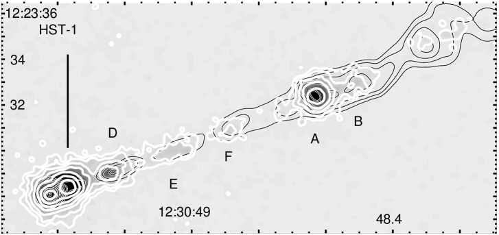
Even when care has been exercised to ensure that the effective beamsizes are close to being the same, relative offsets are sometimes observed between peak emissions at different bands. In fig. 2, we show a comparison of radio and X-ray images of M87. Offsets can be seen for knots D, E, and F (2.5^′′ to 9^′′ from the core). Other cases are the nearest X-ray jet (Cen A, Kraft et al. 2002) and one of the more distant jets, the quasar PKS1127-148 (z=1.18; Siemiginowska et al. 2002).

For synchrotron models of FRI radio galaxies (i.e. with physical offsets of order parsecs, not kpc), a reasonable explanation of the offsets would be that the acceleration region is distributed along the jet and the magnetic field strength is increasing after the initial shock front. Moving downstream, the increasing field strength will lower the maximum energy attainable in subsequent shocks and increase the emissivity. Since the halflives of X-ray emitting electrons are of order a year, whereas the optical and radio emitting electrons would endure ten and 10,000 times longer (respectively), such an acceleration region would naturally produce the observed offsets. No offsets would be expected for a single shock, although the lower frequency emissions could extend further down the jet than the X-ray knot.

A somewhat similar situation exists for the overall structure of a few jets: the brightest X-ray features are close to the nucleus and the knots get fainter moving out the jet. In the case of 3C 273, the optical features have similar intensities but the radio intensities increase as one moves further downstream (the final radio ’knot’ is weak or undetected at optical and X-ray energies). If one were to observe the 3C 273 jet from a great distance with only a few resolution elements for the jet, one would see an offset between the radio and X-ray peaks. Put another way, each small segment of some jets mimics the gross characteristics of the whole (observable) jet. Once again, a natural explanation would be an increasing average field strength as one moves out along the jet.

3.3. Other items needing attention

•

Is there any method to check on the extrapolation to lower $\gamma$ in the electron spectra which is required for IC/CMB models?
•

Are there serious departures from B_eq?
•

Is complex jet structure required? Celotti et al. (2001) suggested the possibility of a fast spine with large $\Gamma$ , surrounded by a sheath with low $\Gamma$ . This obviously provides more latitude to explain observed fluxes in different bands, but is it necessary?
•

How much beaming is there, and where (i.e. in FRI jets? in hotspots?)? Currently we think $\Gamma$ is of order a few in FRI jets, but we don’t really have convincing limits for FRII jets.
•

X-ray emission between discrete knots. If, as seems likely in several jets, there is quasi continuous X-ray emission along the jets, then the standard synchrotron model of acceleration at discrete locations (shocks=knots) fails to explain the emission between knots. Two possibilities are IC/CMB emission from cold pairs (Harris & Krawczynski 2002) and synchrotron emission from distributed acceleration such as might occur from magnetic reconnection along a magnetically dominated jet (Blandford, private communication).

4. Summary

4.1. Goals

It seems reasonable that we may expect progress in understanding a number of jet properties in the not too distant future.

•

Composition: is the major carrier of momentum Ponyting flux, normal plasma, or pair plasma? NB: large $\Gamma$ s at large distances (kpc scales) effectively kills hot pairs.
•

Distribution of $\Gamma$ : refining models, we should be able to obtain reasonable estimates of $\Gamma$ for various jets and for features within jets.
•

Jet Structure: does the fluid follow a helical path or is there a spine plus sheath structure?

4.2. What have we learned so far?

Except for terminal hotspots, all detected X-ray jets are one sided. Therefore, whatever the emission process, Doppler favoritism is operating and we need to include beaming effects. With increased sensitivity, examples of bona fide two sided jets will most likely be found, but this is expected for the small values of the bulk relativistic velocity currently estimated for many FRI radio galaxies.

As reviewed in Harris (2002), X-ray emission from terminal hotspots provides the following conclusions. If the X-rays are synchrotron emission from high energy electrons which are generated by Proton Induced Cascades (rather than the usual high energy tail of a power law distribution), the average magnetic field strength will be large (of order a mG) and hotspots would be good candidates for the origin of UHE cosmic rays.

If the hotspot X-rays come from SSC emission as is commonly accepted, then the fact that the average magnetic field required for SSC is consistent with the conventional equipartition field strength, can be taken as circumstantial evidence that relativistic protons do not contribute to the total particle energy density, and thus are most likely absent.

For the handful of hotspots successfully modeled with SSC, we find $\alpha_{x}~{}\approx~{}\alpha_{r}$ , as expected, and the ratio of photon to magnetic energy densities $\leq~{}0.1$

From X-ray synchrotron emission from knots in jets, $\gamma~{}\approx~{}10^{7}$ and the halflife of the highest energy electrons, $\tau_{\frac{1}{2}}\leq$ a few years. Therefore, X-rays mark the spot of acceleration sites.

From models involving IC/CMB emission, we find the following.

•

Since $\nu_{IC/CMB}=3\times 10^{11}\times\Gamma\times(1+z)\times\gamma^{2}$ , the electrons responsible for the observed X-rays have energies $\gamma$ =30-300 and we may obtain an estimate of the amplitude of the electron spectrum at very low energies.
•

Some jets are relativistic on kpc scales.
•

$\alpha_{x}~{}\approx~{}\alpha_{r}$ (or flatter).

Acknowledgments.

The radio map of M87 was kindly supplied by F. Owen. The work at SAO was supported by NASA contract NAS8-39073 and grant GO2-3144X.

References

Biretta, J. A., Sparks, W. B., and Macchetto, F. 1999, ApJ, 520, 621

Bridle, A.H. 1996, ASP Conference Series 100, 383-394, “Energy Transport in Radio Galaxies”, Hardee, Bridle, & Zensus, eds.

Celotti, A., Ghisellini, G., & Chiaberge, M. 2001, MNRAS, 321, L1

Hardcastle, M. J., Birkinshaw, M., Cameron, R. A., Harris, D. E., Looney, L. W., and Worrall, D. M. 2002, ApJ, 581, 948

Harris, D. E., Biretta, J. A., Junor, W., Perlman, E. S., Sparks, W. B., and Wilson, A. S. 2003, ApJ, (submitted)

Harris, D. E. & Krawczynski, H. 2002, ApJ, 565, 244

Harris, D.E. 2002, in ’Particles and Fields in Radio Galaxies’, ASP Conference Series 250, p.204 R. A. Laing and K. M. Blundell, editors

Kraft, R.P., Forman, W.R., Jones, C., Murray, S.S., Hardcastle, M.J., and Worrall, D.M. 2002, ApJ, 569, 54

Pacholczyk, A.G. 1970, “Radio Astrophysics” W. H. Freeeman, San Franciso

Siemiginowska, A., Bechtold, J., Aldcroft, T.L., Elvis, M., Harris, D.E., and Dobrzycki, A. 2002, ApJ, 570, 543

Tavecchio, F., Maraschi, L., Sambruna, R.M., & Urry, C.M. 2000, ApJ, 544, 23

Wilson, A.S., Young, A.J., & Shopbell, P.L. 2001, ApJ, 547, 740

Wilson, A. S. & Yang, Y. 2002, ApJ, 568,133