CMB power spectrum estimation and map reconstruction with the Expectation - Maximization algorithm

Abstract

We apply the iterative Expectation-Maximization algorithm (EM) to estimate the power spectrum of the CMB from multifrequency microwave maps. In addition, we are also able to provide a reconstruction of the CMB map. By assuming that the combined emission of the foregrounds plus the instrumental noise is Gaussian distributed in Fourier space, we have simplified the EM procedure finding an analytical expression for the maximization step. By using the simplified expression the CPU time can be greatly reduced. We test the stability of our power spectrum estimator with realistic simulations of Planck data, including point sources and allowing for spatial variation of the frequency dependence of the Galactic emissions. Without prior information about any of the components, our new estimator can recover the CMB power spectrum up to scales $l\approx 1500$ with less than 10 % error. This result is significantly improved if the brightest point sources are removed before applying our estimator. In this way, the CMB power spectrum can be recovered up to $l\approx 1700$ with 10 % error and up to $l\approx 2100$ with 50 % error. This result is very close to the one that would be obtained in the ideal case of only CMB plus white noise, for which all our assumptions are satisfied. Moreover, the EM algorithm also provides an straightforward mechanism to reconstruct the CMB map. The recovered cosmological signal shows a high degree of correlation (r = 0.98) with the input map and low residuals.

1 Introduction

Undergoing CMB experiments like BOOMERanG (Netterfield et al. 2002, Rulh et al. 2002), MAXIMA (Hanany et al. 2000), DASI (Halverson et al. 2002), VSA (Grainge et al. 2002), CBI (Mason et al. 2002), ACBAR (Kuo et al. 2002), Archeops (Benoit et al. 2002) and MAP as well as future ones (Planck) will reveal with unprecedented quality the primordial matter fluctuations responsible for the CMB. Very recently the first detection of the E-mode polarization in the CMB has been claimed (DASI, Kovac et al. 2002), which independently supports the structure formation models via gravitational instability. Thanks to these experimental results the fundamental cosmological parameters can be determined with good accuracy.

These experiments will measure also the emission coming from our own Galaxy at mm frequencies as well as the emission due to other galaxies in the same wavebands. On the other hand, galaxy clusters will distort the CMB radiation with an intensity which is proportional to the total mass of the cluster times its temperature. All these components will generate a confusion limit which, together with the intrinsic detector noise, will make very difficult to disentangle which percentage of the observed emission is due to the CMB or to the other components. Several component separation methods have been proposed so far in the literature: multifrequency Wiener filter (MWF, Tegmark and Efstathiou 1996, Bouchet and Gispert 1999), maximum entropy methods (MEM, Hobson et al. 1998, Vielva et al. 2001b; extended to the sphere in Stolyarov et al. 2002, Barreiro et al. 2003), independent component analysis (ICA, Baccigalupi et al. 2000, Maino et al. 2002), blind Bayes (Snoussi et al. 2001).
Although there are some similarities and differences between the previous methods, all of them share a common aspect: they try to separate all the components simultaneously. For this purpose, these methods usually need to assume some a priori information about the components. Thus, if the different components have different frequency dependencies, then, by examining the data at different frequencies it is possible to distinguish (at a certain level) the different components. Or, if we know the correlation function of the components (or their power spectrum) and each one is significantly different from each other, then, it is also possible to distinguish (again at a certain level) the components since their modes will behave differently in the Fourier space. If one knows both, the frequency dependence and the power spectrum, then the component separation improves dramatically since now it is possible to combine the information in the different channels by correlating the Fourier modes with a correlation given essentially by the frequency dependence of each component and its power spectrum. This approach has proved to be very useful if the frequency dependence and power spectrum of the components are known.
It is interesting to explore what kind of information can be obtained when no prior information is assumed about none of the components. In some cases we simply do not know the priors (as it happens in the case of the free-free emission or the spinning dust). On the other hand, if we assume something about the components which is not accurate but an approach, then we are intrinsically introducing some bias in our final result. If, after the component separation, we end up with a biased estimate on, at least, one of the components, this will have an effect on some (if not all) of the other components which must absorb that bias in order to obey the constraint that the sum of all the components must be equal to the original data. This very last point is one of the risks of the simultaneous component separation methods.
Another assumption usually made is that the components are, one from each other, statistically independent. This assumption is not true for several of the components (like the Galactic ones). This assumption can be a source of systematic errors. Other typical assumption is that the probability distribution function (pdf) of the individual components is a Gaussian. This is false for components like the point sources, the Sunyaev-Zeldovich (SZ) and the Galactic emissions where the true pdf has a bell-shape with a long tail towards positive values (negative for the SZ for frequencies below 217 GHz). This assumtion will be somewhat relaxed in this work by assuming that the combined foreground emission plus instrumental noise is Gaussian distributed in Fourier space, instead of assuming it for each individual component. We will study the effect of this assumption at different scales. At those scales where the assumption is less justified solutions will be proposed to reduce the effect.

In a recent paper (Delabrouille et al. 2002) the authors have used the Expectation-Maximization (EM) algorithm to minimize a spectral matching criterion. They consider the problem of component separation with four components, CMB, SZ effect, dust and instrumental noise. In that work, the authors have shown that this is an interesting alternative to estimate jointly the frequency dependence and spatial power spectra of the components. This method allows to introduce certain degrees of freedom or free parameters in the problem. These free parameters can be determined after iterating an expectation-maximization process.

In the work presented here, we will explore this direction but in a much more simplified manner focusing only on the estimation of the power spectrum and the map reconstruction of the CMB but including more components than in the previous work and doing no assumptions at all about the power spectrum or frequency dependence of any of the components. In addition to the diffuse foregrounds, we also will study the effect of point sources which were not considered in the previous work.

The approach presented in this paper can be extended to determine jointly the CMB and the SZ components. The physics of these two emissions is well known, in particular their frequency dependence. Therefore, no prior assumptions about their frequency behaviour is required. In addition, these two components –together with the point sources one– are the most important signals from the cosmological point of view. Several works have already been presented to determine the SZ (Herranz et al. 2001b,c; Diego et al. 2002) and the point sources emissions (Tegmark & Oliveira-Costa 1998; Cayón et al. 2000; Sanz et al. 2001; Vielva et al. 2001, 2003; Chiang et al. 2002; Hobson & McLachlan 2002) from microwave images. Our aim for the future will be to develop a method based on the EM algorithm combined with a point source detection technique, to recover simultaneously the three cosmological emissions.

The paper is organized as follows. In Section 2, we summarize the key ideas behind the EM algorithm. In Section 3 we apply the EM algorithm to the problem of determining an estimator of the CMB power spectrum. The main results are shown in Section 4. These results are compared with the ones which would be obtained in the ideal case when only CMB and white noise are considered. Finally, the conclusions are given in Section 5.

2 The Expectation-Maximization algorithm

In this section we will present an alternative method which will be useful to get a robust estimate of the power spectrum of the CMB. We will also present a single iterative expression for the new estimator of the CMB power spectrum. This estimator can be used directly with multifrequency microwave data to give a fast, accurate and robust estimate of the power spectrum of the CMB.
EM is an algorithm useful when there is a many-to-one mapping. That is, several variables are combined together to give one observed quantity. This is exactly our problem where the complete data are just the different components (Galactics, extragalactics, CMB and noise) and the observed quantity is just the projection of all of them in one of the channels (data on the receiver). EM allows to introduce degrees of freedom (or free parameters) in the pdf of the complete data and then look for the best parameters by maximising the expected value of that pdf given the observations.
The advantage of this algorithm in our problem is obvious. Since part of the information about the components is unknown, we can parametrise this unknown information as free parameters in the pdf of the complete data. Then, the maximization process will give us the best set of free parameters given the data.

The EM algorithm (Dempster et al. 1977) provides an iterative procedure for computing maximum likelihood estimates (MLEs) in situations where the observed data vector, $\bf{d}$, is viewed as being incomplete. $\bf{d}$ is an observable function of the so-called complete data ${\bf x}$ (see e.g. McLachlan and Krishnan 1997). Let’s denote by ${\bf f_{i}(d|p)}$ the pdf’s of the incomplete data $\bf d$ and by ${\bf f(x|p)}$ the pdf of ${\bf x}$. The vector ${\bf p=(p_{1},....,p_{N})}$ will contain the $N$ unknown parameters. The complete-data log likelihood function that could be formed for ${\bf p}$ if ${\bf x}$ were fully observable is given by

$$\log L(\bf p)=\log f(\bf x|\bf p).$$ (1)

Instead of observing ${\bf x}$, we observe ${\bf d}$, with many-to-one mapping from ${\bf x}$ to ${\bf d}$ (i.e ${\bf d=d(x)}$). It follows that

$${\bf{f_{i}(d|p)=\int_{X_{d}}}{\bf{f(x|p)dx}}}$$ (2)

where ${\bf X_{d}}$ is the sub-space of ${\bf x}$ defined by ${\bf d=d(x)}$.
The EM algorithm approaches the problem of solving the incomplete-data likelihood, ${\log\mathcal{L}\rm(\bf p)=\log f_{i}(d|p)}$, indirectly by proceeding iteratively in terms of the complete-data log likelihood function, $logL({\bf p})$. As it is unobservable, it is replaced by its conditional expectation given ${\bf d}$, using the current fit for ${\bf p}$. More specifically, the EM algorithm consists of two steps: Expectation (E-step) and Maximization (M-step). On the j+1 iteration, these steps are as follows:

$\bullet$ E-step: Calculate the quantity $Q({\bf p|\bf p^{j}})$, defined as $Q({\bf p|\bf p^{j}})=E\{\log L({\bf p)|\bf d,\bf p^{j}}\}$.

$\bullet$ M-step: Choose ${\bf p^{j+1}}$ to be the value that maximises $Q({\bf p|\bf p^{j}})$; that is, $Q({\bf p^{j+1}|\bf p^{j}})=\max[Q({\bf p|\bf p^{j}})]$.

That is, in the first step we compute the expected value of the log of the complete pdf given the data and an estimate of the parameters (${\bf p^{j}}$). In the second step we look for the values of the parameters which maximise the previous expected value. At this step, we have to maximise with respect to each one of the parameters ($p^{j}(i)$). This can be done by just setting the first derivative of $Q({\bf p;\bf p^{j}})$ with respect to that parameter to $0$ and solving for $p^{j}(i)$.
This is an iterative process which can be started with an arbitrary choice for the parameters in the first step, ${\bf p^{o}}$. The EM algorithm assure us that at every step the likelihood $\mathcal{L}\rm({\bf p})$ is increased. The method will converge to the optimal set of parameters, ${\bf p}$, in a number of steps which will depend on the nature of the problem and on the initial election for the first iteration, ${\bf p^{o}}$.

In this paper, we will consider a simple case where we allow the covariance in Fourier space of the CMB signal (or power spectrum) to be a free parameter.
We will apply the EM algorithm in order to determine that free parameter (the power spectrum of the signal). This case can be extended to include more free parameters in the analysis as it is shown in Delabrouille et al. (2002).

3 EM applied to CMB experiments

If we know the frequency dependence of one of the components, then we can express the signal at a given frequency as:

$${\bf S}({\bf n},\nu)={\bf A}({\bf n},\nu)\otimes\Big{(}{\bf f}(\nu)s({\bf n})\Big{)}$$ (3)

where $s({\bf n})$ is the spatial pattern of the signal we want to estimate, ${\bf f}(\nu)$ is the frequency dependence of the signal (including the band-with), and ${\bf A}({\bf n},\nu)\otimes$ accounts for the convolution with the antenna beam of the experiment and its frequency response.
The data at different frequencies, ${\bf d}(\nu)$, can be expressed as a sum of the signal plus some other contributions.

$${\bf d}({\bf n},\nu)={\bf S}({\bf n},\nu)+{\bf\xi}({\bf n},\nu).$$ (4)

The residual ${\bf\xi}({\bf n},\nu)$ includes all the other components, i.e. Galactic and extragalactic components convolved with the corresponding beam plus the corresponding instrumental noise. Due to the antenna and frequency convolution in ${\bf A}({\bf n},\nu)\otimes$, it is easier to work in Fourier space where this convolution is just a product of the Fourier modes which are uncorrelated provided the field is homogeneous and isotropic. Therefore, the previous equation should be rather expressed in Fourier space as:

$$d_{\nu}({\bf k})=A_{\nu}(k)f_{\nu}s({\bf k})+\xi_{\nu}({\bf k}).$$ (5)

If the experiment has $m$ different channels, then we have an observation for each channel. That is, we have the vector of observations ${\bf d}=(d_{1},d_{2},...,d_{m})$ for each Fourier mode ${\bf k}$. And we can write:

$${\bf d}={\bf R}s+{\bf\xi}$$ (6)

where, ${\bf R}$ is the response vector containing $m$ elements. Each element of ${\bf R}$ is just the product of the antenna and the frequency response of the instrument times the frequency dependence of the signal,

$$R_{\nu}=A_{\nu}f_{\nu}.$$ (7)

In the case in which the signal is the CMB then $f_{\nu}=1\ \ \forall~{}\nu$. From eqn. 6 we can express the residual as

$${\bf\xi}={\bf d}-{\bf R}s.$$ (8)

The basic starting point when applying EM is to define the pdf of the complete data. In our case the complete data are all the components plus the multifrequency observations $\mathbf{d}$. We will focus on the problem in which the complete data can be divided in just two elements. The two elements are the CMB signal we want to estimate $s$ and the observed data $\mathbf{d}$ (or equivatently the residual $\xi$, noise plus rest of components; see below). By doing this, the nature of our problem reduces drastically since we only have to make assumptions about two elements.
Furthermore, the residual and the signal can be considered as independent. In terms of the probability, the pdf of the complete data is:

$${\bf f}({\bf x}|{\bf p})={\bf P}(s,{\bf d}|{\bf p})={\bf P}(s,{\bf\xi}|{\bf p})={\bf P}(s|{\bf p_{A}}){\bf P}({\bf\xi}|{\bf p_{B}})$$ (9)

where ${\bf p}=\bigcup{\bf p_{A}}{\bf p_{B}}$ with ${\bf p_{A}}$ and ${\bf p_{B}}$ unknown parameter sets for the pdf’s of $s$ and ${\bf\xi}$. The second equality follows from the transformation $(s,{\bf d})\rightarrow(s,{\bf\xi})$ whose Jacobian is equal to one (see equation 5). It is important to note that, in oppossition to other methods, our assumption about independence of the elements ($s$ and ${\bf\xi}$) is well justified. No relation is expected between the CMB and the other foregrounds (except maybe the SZ effect which could be weakly related to the CMB through the ISW effect).

Once we have established that the two elements are independent, we need a clue about the specific form of the individual probabilities, ${\bf P}(s|{\bf p_{A}})$ and ${\bf P}({\bf\xi}|{\bf p_{B}})$. If the CMB is close to a Gaussian variable (and we know it is), then the pdf of the CMB in Fourier space can be approached by:

$${\bf P}(s|{\bf p_{A}})\equiv{\bf P}(s)\propto P(k)^{-1}exp(-\frac{s^{2}}{P(k)})$$ (10)

where $P(k)$ is the power spectrum of the CMB: the parameter to be estimated.
The pdf of the residual (${\bf\xi}$) can be modelled as

$${\bf P}({\bf\xi}|{\bf p_{b}})\equiv{\bf P}({\bf\xi})\propto exp(-\boldmath{\xi}C^{-1}\boldmath{\xi}^{{\dagger}})$$ (11)

where $C^{-1}$ is the inverse of the correlation matrix of the residual. $C$ is an $n\times n$ matrix ($n=$ number of channels). This correlation matrix is not diagonal if there are some correlations in the residuals between the different frequency channels. The elements of $C$ are the power (diagonal) and cross-power (off-diagonal) spectra of the residuals at each channel which can be given as a function of the $P(k)$ (see below).
We have assumed in equation (11) that the residuals are Gaussian distributed. This assumption is not as strong as assuming that each component is Gaussian distributed. The sum of several non-Gaussian distributions tends to a more Gaussian one. In the limit of a sum of infinite independent components the central limit theorem assures that the resulting distribution is Gaussian. In any case Gaussianity can be a good approach at scales where the instrumental noise dominates the residuals. The most critical situations for the validity of this assumption appear at large and small scales since, at least for some channels, they are dominated by the Galactic components and the compact sources, respectively. Solutions for these problems will be proposed in the next sections.

In the previous relations for the individual pdf’s appear the power spectra of the signal and the residual. In a real situation these quantities are unknown. This is the reason why we apply EM. We can introduce the unknown CMB power spectrum, $P(k)$, as the uncertainty in our problem. In order to apply EM and estimate this free parameter we have to calculate the expected value $Q({\bf p}|{\bf p^{j}})$ which is just an integral:

$$Q({\bf p|p^{j}})=\int log{\bf P}(s,{\bf d}|{\bf p}){\bf P}(s|{\bf d},{\bf p^{j}})ds.$$ (12)

The only thing we need to know to calculate $Q({\bf p}|{\bf p^{j}})$ are the probabilities ${\bf P}(s|{\bf d})$ and ${\bf P}(s,{\bf d})$. By Bayes we know that:

$${\bf P}(s|{\bf d})=\frac{{\bf P}(s,{\bf d})}{{\bf P}({\bf d})}$$ (13)

where ${\bf P}({\bf d})$ can be obtained just by marginalising ${\bf P}(s,{\bf d})$ over $s$:

$${\bf P}({\bf d})=\int{\bf P}(s,{\bf d})ds$$ (14)

and ${\bf P}(s,{\bf d})$ can be obtained through the chain rule:

$${\bf P}(s,{\bf d})={\bf P}(s,{\bf\xi})J\left(\frac{s,{\bf\xi}}{s,{\bf d}}\right).$$ (15)

By taking equation (5), one can prove that the Jacobian in the previous expression is equal to one, as it was commented above, so we have:

$${\bf P}(s,{\bf d})={\bf P}(s,{\bf\xi})$$ (16)

where (see equation 9),

$${\bf P}(s,{\bf\xi})\propto P(k)^{-1}exp(-\frac{s^{2}}{P(k)})exp(-{\bf\xi}C^{-1}{\bf\xi}^{{\dagger}})$$ (17)

where the term, $P(k)$, accounts for our free parameter in ${\bf P}(s|{\bf p_{A}})$ (see equation 10) and the second term was taken from equation (11). We remark that the covariance matrix $C$ also depends on the free parameter $P(k)$, as it will be discussed below.

Now it is easy to compute the terms, ${\bf P}({\bf d})$, ${\bf P}(s|{\bf d})$, and finally $Q(P(k)|P(k)^{j})$:

$${\bf P}({\bf d})\propto\frac{exp\Big{(}-{\bf d}C^{-1}{\bf d}^{{\dagger}}+({\bf d}C^{-1}{\bf R}^{{\dagger}})^{2}/F_{1}\Big{)}}{P(k)|C|^{1/2}F_{1}}$$ (18)

where we have expressed ${\bf\xi}$ in terms of ${\bf d}$ and $s$ (see eqn. 8).

$${\bf P}(s|{\bf d})\propto F_{1}exp\left(-F_{1}\Big{|}s-\frac{{\bf d}C^{-1}{\bf R}^{{\dagger}}}{F_{1}}\Big{|}^{2}\right)$$ (19)

where,

$$F_{1}={\bf R}C^{-1}{\bf R}^{{\dagger}}+P(k)^{-1}.$$ (20)

Finally the expected value of the log of the complete pdf (equation 12) is:

$$Q(P(k)|P(k)^{j}) = -log(P(k))-\frac{1}{2}log|C|-{\bf d}C^{-1}{\bf d}^{{\dagger}}$$

$$- F_{1}<|s|^{2}>+2\mathbf{d}C^{-1}{\bf R}^{{\dagger}}<s>+const.$$

where :

$$<s>=\frac{{\bf d}C^{-1}{\bf R}^{{\dagger}}}{F_{1}}$$ (22)

$$<|s|^{2}>=\frac{1}{F_{1}}\left(1+\frac{|{\bf d}C^{-1}{\bf R}^{{\dagger}}|^{2}}{F_{1}}\right).$$ (23)

Equation (22) is nothing more than multifrequency Wiener filter computed with the CMB power spectrum at iteration $j$. This is an expected result since Gaussianity for the signal and residuals have been assumed. Similarly, the signal variance at each $k$ $<|s|^{2}>$ is also computed with $P(k)^{j}$ at iteration $j$. At this point it is important to note that in eq. (3) the dependence on $P(k)$ appears explicitly in the first term and also in the fourth one through the function $F_{1}$. Moreover, since we do not know the residuals the $P(k)$ dependence is also present in the other terms through the residual covariance matrix,

$$C^{\nu\mu}=P_{\bf\xi}^{\nu\mu}(k)=P_{\bf d}^{\nu\mu}(k)-R^{\nu}R^{\mu}P(k)$$ (24)

where $P_{\bf\xi}^{\nu\mu}(k)$ and $P_{\bf d}^{\nu\mu}(k)$ are the residual and data cross-power spectra after convolution with the corresponding antenna response whereas $P(k)$ is the unconvolved CMB power spectrum to be determined.

In the maximisation step, the value of $P(k)^{j+1}$ that maximises $Q(P(k)|P(k)^{j})$ should be found. Finding the maximum is not a trivial task given the complicated dependence on $P(k)$. In order to facilitate the finding we consider the residual covariance matrix, $C^{\nu\mu}$, constant in the M-step (but changing with $P(k)$ in the E-step). With this simplification, we can easily find the analitical solution for the maximum by differentiating $Q(P(k)|P(k)^{j})$ with respect to $P(k)$ and equating to zero. We find the not so surprising result:

$$P(k)^{j+1}=<|s|^{2}>.$$ (25)

The previous equation is the main result of EM. $<|s|^{2}>$ is given by equation (23) computed with the value of $P(k)$ at iteration $j$. By iterating equation (25), which only depends on the data, the response vector and the CMB power spectrum obtained in the previous iteration, we can get an estimate of the power spectrum of the underlying signal. The final step after the EM estimation of the signal power spectrum at each $k$, is to recover the CMB map by applying eqn. 22, the multifrequency Wiener filter derived within the EM framework.

Finally, this method can be easily extended to determine jointly the CMB and the SZ emissions, since they are almost uncorrelated and the frequency dependence of the SZ is also very well known. In addition, the method can be implemented with more realistic (non-Gaussian) pdfs to model the signal distributions as well as the residuals. We will study these extensions of the method in a future work.

4 Results

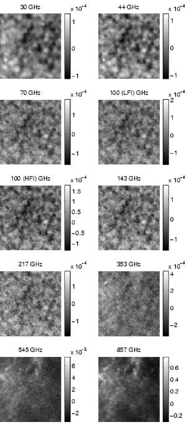
Figure 1: Realistic simulations of the data, covering a $12.8^{o}\times 12.8^{o}$ patch, expected from the 10 Planck channels. The RMS amplitude (at 353 GHz and in $\Delta T/T$ thermodinamic temperature units) is $4.26\times 10^{-5}$ for the CMB, $5.16\times 10^{-6}$ for the PS emission, $3.93\times 10^{-6}$ for the SZ contribution, $5.82\times 10^{-5}$ for the thermal dust, $3.23\times 10^{-7}$ for the free-free radiation, $1.46\times 10^{-6}$ for the synchrotron emission and it is almost negligible in the case of the spinning dust (see text).

In this section, we present the results that have been obtained for the CMB power spectrum determination. Firstly, we briefly describe the simulated data that have been used in this work, accounting for the most important contributions to the microwave sky. Then, we present our CMB power spectrum estimation. An improvement at small scales is achived by using a very useful tool for subtracting the brightest point sources: the Mexican Hat Wavelet.

Finally, we applied our estimator to an ideal data set, where the Gaussian assumption for the residuals is satisfied. This exercise is highly interesting, since it shows the robustness of our estimator: the results achieved in this idealistic case are only slightly better than the ones obtained in the reslistic situation.

4.1 Simulated data

Frequency	FWHM	Pixel size	$\sigma_{noise}$
(GHz)	(arcmin)	(arcmin)	$(10^{-6})$
857	5.0	1.5	22211.10
545	5.0	1.5	489.51
353	5.0	1.5	47.95
217	5.5	1.5	15.78
143	8.0	1.5	10.66
100 (HFI)	10.7	3.0	6.07
100 (LFI)	10.0	3.0	14.32
70	14.0	3.0	16.81
44	23.0	6.0	6.79
30	33.0	6.0	8.80

Table 1: Experimental constrains at the 10 Planck channels. The antenna FWHM is given in column 2 for the different frequencies (a Gaussian pattern is assumed in the HFI and LFI channels). Characteristic pixel sizes are shown in column 3. The fourth column contains information about the instrumental noise level, in $\Delta T/T$ per pixel.

To show the power of our approach we will apply our estimator (eqn. 25) to realistic simulations. They consider the expected levels of the instrumental white noise and resolution characteristics of the 10 Planck mission channels at 30, 44, 70, 100 (Low and High Frequency Instrument, LFI and HFI), 143, 217, 353, 545 ad 857 GHz (see Table 1). In addition, we use state of the art simulations of the different galactic and extragalactic components, together with the pure CMB signal.

Within the first ones, we have taken into account the synchrotron, free-free, spinning and thermal dust contributions. The first one has been simulated using the all-sky pattern provided by Giardino et al. (2002) including both, temperature and spectral index templates. The free-free emission is very poorly known. Recent experiments focusing on the H-$\alpha$ detection, like Southern H-$\alpha$ Sky Survey (SHASSA, Reynolds & Haffner, 2000) and the Wisconsin H-$\alpha$ Mapper project (WHAM, Gaustad et al. 2001), will produce all-sky surveys that could be used as free-free templates. However, since these data are not available at the present time, we have used the correlation between dust and free-free emissions proposed by Bouchet et al. (1996) as spatial template, and a power law, $I_{\nu}\propto{\nu}^{-0.16}$, to describe the frequency dependence. We have also included the spinning dust emission –proposed by Draine & Lazarian (1998) as a possible explanation for the anomalous Galactic emission found by CMB experiments like COBE (Kogut 1999) or Saskatoon (Oliveira-Costa et al. 1997). Very recently, a tentative confirmation of that emission has been claimed (Finkbeiner et al. 2002). The simulation of that emission has been carried out using the frequency dependence proposed by Draine & Lazarian (1998) and using the thermal dust component as an spatial template, since both dust emissions are strongly correlated through the neutral hydrogen column density ($N_{H}$). Finally, thermal dust emission has been also simulated, using the best model proposed by Finkbeiner et al. (1999) to fit the FIRAS, IRAS and DIRBE data, consisting of two grey-bodies with mean temperatures of 16.2 K and 9.4 K and emissivities 2.70 and 1.67, respectively.

The simulated extragalactic foregrounds are the thermal Sunyaev-Zel’dovich effect (SZ) and radio and infrared point sources. The SZ was performed following the Diego et al. (2001) model for a flat $\Lambda$CDM Universe with $\Omega_{m}=0.3$ and $\Omega_{\Lambda}$ = $0.7$. The point sources correspond to the Toffolatti et al. (1998) model for the same Universe, including radio flat-spectrum and infrared sources. We refer to that paper for details.

Finally, the CMB signal was simulated using the $C_{l}$’s provided by the CMBFAST code (Seljak & Zaldarriaga, 1996) for the same cosmological model and assuming Gaussian fluctuations. We would like to remark that synchrotron, thermal dust and the point source emissions have been simulated using a frequency dependence which varies with the sky position. The simulated maps covering a patch of the sky of $12.8^{o}\times 12.8^{o}$, as seen by the 10 Planck channels, are shown in figure 1.

Figure 2: Recovered power spectrum by our estimator. The solid line is the true power spectrum and the dotted and dashed lines represent the recovered power spectrum obtained by our estimator directly from the data and the one recovered after previous subtraction of the brightest point sources, respectively. P(k) is in $\Delta T/T$ units. Notice that the multipole $l$ is related to the wave number $k$ through $l\approx 28k$.

Figure 3: Relative error in % of the recovered power spectrum by our estimator (dash-dotted line). For comparison we have plotted the errors obtained by our estimator in the ideal situation when only CMB and instrumental white noise are present in the data (see text).

Figure 4: Relative error in % of the recovered power spectrum by our estimator after the brightest point sources have been removed in all the channels (dash-dotted line). For comparison in the solid line we have plotted the errors obtained by our estimator in the ideal situation when only CMB and instrumental white noise are present in the data (see text).

4.2 A simple choice for the correlation matrix

In order to estimate the power spectrum of the CMB through eqn. (25) we still have to iterate a relatively complex expression containing a cocient of polynomials of order twice the number of channels and involving many terms. To further simplify the convergence of that equation we will only consider the diagonal terms of the covariance matrix, making zero the other non-diagonal elements. This assumption does not take into account the correlations among the residuals at different channels due to the Galactic components and compact sources. The former are reflected at the low $k$-modes and their effect can be reduced by performing a simple Galactic subtraction as the one proposed by Diego et al. (2002). The later have their impact at intermediate (e.g. radio sources observed in the lowest resolution channels) and large $k$-modes (e.g. infrared sources). However, as it will be shown below, once the brightest point sources are subtracted from the maps, the contribution of the remanent point sources is low enough to make their effect significantly smaller.

In figure 2 we present our results for the 10 Planck channels using the data obtained from the combination of the simulated components as described above (figure 1). The comparison of the recovered spectrum with the true one shows a good agreement until $k$ values larger than the one corresponding to the best antenna channels and the results start to be dominated by the deconvolved noise.

In order to better appreciate the differences, we show in figure 3 the relative error, $(P_{r}(k)-P_{t}(k))/P_{t}(k)$ %, where $P_{r}(k)$ is the estimator of equation 25.

In both large and relatively small scale range (small and relatively large $k$) our estimator finds a reasonably good estimation of the true power spectrum. The error is small (less than 10 %) up to scales $k\approx 55$ (which corresponds to $l\approx 1500$). The effect of only considering the diagonal terms of the residual covariance matrix is small (see also the comparison with the ideal case below). This fact proves the applicability of our assumption for the microwave data since our method is not very sensitive to the cross-correlations of the different channels.

At very small scales ($k>45$ or $l>1300$) the signal is below the noise level and the error bars grow quickly. Our estimator shows a clear bias toward higher values (we recover more power than the true one). This implies that some of our assumptions are wrong at these small scales. The Gaussianity assumption is a good approximation in Fourier space at large $k$-modes (because of the dilution in many modes of the clear non-Gaussian features appearing in the real space). However, the uncorrelation assumption among frequency channels is a source of bias at these scales, since the bright point sources are strongly correlated. We have checked this point by removing the brightest point sources (but leaving the galaxy clusters and the weak point sources in the residual). We have used the Mexican Hat Wavelet (MHW) technique proposed by Vielva et al. (2001a) for removing point sources above the fluxes determined by the so-called $50\%$ error criterion used in that paper. These fluxes correspond to those detection limits above which the maximum percentage of spurious detection is $5\%$, being a detection spurious if the error in the amplitude estimation is larger than $50\%$. After the subtraction, we applied our estimator to these new point-source-free maps. The final result is shown in figure 4. The effect of removing the brightest point sources is evident now. This result clearly shows how the bias can be corrected by removing the compact sources. The relative error does not change significantly after removing the point sources but the estimator is able to go up to scales $k=60$ ($l\approx 1700$) with relative error $<10\%$. The error is smaller than $50\%$ below $k=75$ ($l\approx 2100$).

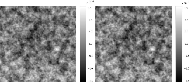
Figure 5: Left: CMB map reconstruction by our method (equation 22) using the recovered power spectrum obtained after previous subtraction of the brightest point sources. Right: Input CMB map. Both maps have been convolved with a Gaussian beam of FWHM = 5 ’

4.3 Comparing with an ideal situation

It is interesting to answer whether or not the above results are close to the most optimistic case where all our assumptions are right (Gaussianity and $C$ diagonal). We will check this point in the simple (but unrealistic) case where our data consist only of CMB signal plus the corresponding instrumental noise for each channel. In this simple case, our assumption of Gaussianity is right since both CMB and noise are Gaussian. The correlation matrix of the residual, $C$, will be exactly diagonal with the elements being the power spectrum of the data minus the CMB power spectrum convolved with the antenna corresponding to each channel.

In figures 3 and 4 we show the performance of the EM estimator in this ideal case (CMB plus noise) after combining the 10 Planck channels. The result is surprisingly very similar to the one obtained in the realistic case where the brightest point sources have been subtracted (figure 4). This test shows how the EM estimator is extremely robust and can give results very close to the most optimal one.

4.4 Map reconstruction

Using the expression given in equation 22 and the estimated power spectrum $P_{r}(k)$, we are able to recover the CMB map. As it was pointed out in Section 3, due to the Gaussianity assumptions, equation 22 is nothing more than multifrequency Wiener filter (MWF). Hence, our map reconstruction is a MWF focused on the CMB recovery. Let us remark that this approach differs from the traditional MWF already used in the microwave sky recovery (e.g., Tegmark & Efstathiou 1996, Bouchet & Gispert 1999 and Hobson et al 1998). These works were focused on the all components separation, whereas our approach is devoted to reconstruct just the CMB signal. Even more, whereas the traditional approaches require previous knowledge of the power spectra (not only the CMB one, but also the power spectra of the foregrounds), the CMB power spectrum is a result of the blind EM method. This and the non requirement of any prior knowledge about the frequency dependence of the components, are the strongest points of the blind methods. In figure 5 we present the CMB map reconstruction (left) together with the input one (right). Both maps have been convolved with the best Planck resolution (FWHM = 5’). The correlation between the input and recovered CMB maps is very good $r=0.98$ (figure 6), whereas the slope of the best straightline fit is 0.97. The residual CMB is dominated by the Galactic dust emission, since it is the most important foreground at low $k$-modes. Hence, by performing a simple dust subtraction as the one proposed by Diego et al. (2002) –which basically consists in using the 857 GHz channels as a dust template to be subtracted from the others channels– a significant improvement in the CMB map reconstruction is achieved, being the RMS of the residual map lower than $15\%$.

5 Conclusion

We have presented an efficient estimator (eqn. 25) of the CMB power spectrum. Our estimator is based on the EM algorithm and does not make use of any prior information whatsoever about any of the components. This renders satisfactory results, since we are able to recover the power spectrum up to $l\approx 1500$ with less than 10% error. This limit can be improved if we remove the brightest compact sources, for instance applying the MHW technique poposed by Vielva et al. (2001a). After point source removal the estimator can recover the power spectrum up to $l\approx 1700$ with less than 10% error and up to $l\approx 2100$ with less than 50% error.

Our results are very close to the optimal case when all our assumptions are satisfied (only CMB and instrumental noise are included in the simulations), as can be seen in figure 4. There are several CMB power spectrum estimations in the literature, given for different component separation techniques, like Bayesian methods (MEM: Hobson et al. 1998 and Stolyarov et al. 2002; and MWF: Tegmark & Efstathiou 1996 and Bouchet & Gispert 1999) and blind source separation algorithms (ICA and FastICA: Baccigalupi et al. 2000 and Maino et al. 2002; and Multi-Detector Multi-Component analysis: Delabrouille et al. 2002). This work provides a CMB power spectrum that is comparable to or even better than the previous ones, being more robust than those, since previous knowledge about the underlying components is not requiered (contrary to the Bayesian methods) and simulations used in previous works are significantly more idealised than the ones used in this work (e.g., lack of spatial variation of the frequency dependence for several components; absence of some of the components, like point sources or some Galactic foregrounds). On the other hand, our simulations account for the previous limitations including all the major microwave emissions and allowing for spatial variation of the frequency dependence. Finally, our method is able to reconstruct the CMB map using the estimated power spectrum and the MWF given in equation 22. Let us remark that the MWF is obtained when the Gaussianity hypothesis is assumed, whereas the EM algorithm provides a more general procedure for component separation. That hypothesis will be explored in a future work by including more realistic distributions for the different components. In addition, we are working on a jointly determination of the cosmological signals (CMB, SZ and point sources) using the EM algorithm and a point source detection tool. Finally, an extension of this algorithm to the sphere is straightforward and will be studied soon.

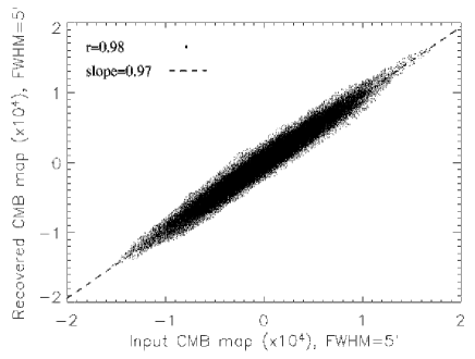
Figure 6: Correlation between the input and recovered CMB maps. The best strightline fit is also plotted.

References

- [1] Baccigalupi, C., Bedini, L., Burigana, C., De Zotti, G., Farusi, A., Maino, D., Maris, M., Perrota, F., Salerno, E., Toffolatti, L., Tonazzini, A., 2000, MNRAS, 318, 769
- [2] Barreiro, R.B., Hobson, M.P., Banday, A.J., Lasenby, A.N., Stolyarov, V., Vielva, P., Górski, K.M., 2003, MNRAS, submitted
- [3] Benoit, A. et al., 2002, A&A in press, astro-ph/0210306
- [4] Bouchet, F. R., Gispert, R. & Puget, J. L., 1996 in Drew, E., ed., Proc. AIP Conf. 384, The mm/sub-mm foregorunds and future CMB space missions. AIP Press, New York, p. 255
- [5] Bouchet, F. R. & Gispert R., 1999, NewA, 4, 443
- [6] Cayón, L., Sanz, J. L., Barreiro, R. B., Martínez-González, E., Vielva, P., Toffolatti, L., Silk, J., Diego, J. M. & Argüeso, F., 2000, MNRAS, 315, 757.
- [7] Chiang, L. Y., Jogensen, H. E., Naselsky, I. P., Naselsky, P. D., Novikov, I. D. & Christensen, P. R., 2002, MNRAS, 335, 1054
- [8] Delabrouille J., Cardoso J.F., Patanchon G. 2002 MNRAS submitted. Preprint astro-ph/0211504.
- [9] Dempster, A.P., Laird, N.M., Rubin, D.B., 1977, Journal of the Royal Statistical Society B, 39, 1.
- [10] Diego, J. M., Martínez-González, E., Sanz, J. L., Cayón, L. & Silk, J., 2001, MNRAS, 325, 1533.
- [11] Draine, B. T. & Lazarian, A., 1998, ApJ, 494, L19.
- [12] Finkbeiner, D. P., Davis, M. & Schlegel, D. J., 1999, ApJ, 524, 867
- [13] Finkbeiner, D. P., Schlegel, D. J., Frank, C. & Heiles, C., 2002, ApJ, 566, 898
- [14] Gaustad, J. E., McCullough, P. R., Rosing, W. & Van Buren, D., 2001, PASP, 113, 1326
- [15] Grainge, K. et al., 2002, MNRAS submitted, astro-ph/0212495
- [16] Halverson, W., et al., 2002, ApJ, 568, 38
- [17] Hanany, S., et al. 2000, ApJ, 545, L1
- [18] Herranz, D., Gallegos, J. E., Sanz, J. L. & Martínez-González, E., 2002a, MNRAS, 334, 533
- [19] Herranz, D., Sanz, J. L., Barreiro, R. B. & Martínez-González, E., 2002b, ApJ, 580, 610
- [20] Herranz, D., Sanz, J. L., Hobson, M. P., Barreiro, R. B., Diego, J. M., Martínez-González, E. & Lasenby, A. N., 2002c, MNRAS, 336, 1057
- [21] Hobson M.P., Jones A.W., Lasenby A.N., Bouchet F.R., 1998, MNRAS, 300, 1.
- [22] Hobson, M. P., & McLachlan, C., 2002, MNRAS, submitted, astro-ph/0204457
- [23] Kovac, J., Leitch, E. M., Pryke, C., Carlstrom, J. E., Halverson, N. W. & Holzapfel, W. L., 2002, astro-ph/0209478
- [24] Kogut, A., 1999, ASP Conf. Ser. 181: Microwave Foregrounds, p. 91.
- [25] Kuo, C. L. et al., 2002, astro-ph/0212289
- [26] Maino, D., Farusi, A., Baccigalupi, C., Perrotta, F., Banday, A. J., Bendini, L., Burigana, C., De Zotti, G., Górski, K. M. & Salerno, E., 2002, MNRAS, 334, 1, 53
- [27] Mason, B.S. et al., 2002, ApJ, submitted, astro-ph/0205384.
- [28] McLachlan, G. & Krishnan, T.,1997, The EM Algorithm and Extensions. Wiley series in Probability and Statistics
- [29] Netterfield, C. B., et al., 2002, ApJ, 571, 604
- [30] de Oliveira-Costa, A., Kogut, A., Devlin, M. J., Netterfield, C. B., Page, L. A. & Wollack, E. J., 1997, ApJL, 482, L17.
- [31] Reynolds, R. J. & Haffner, L. M., 2000, ASP Conference Series, IAU Symposium #201, in press
- [32] Rulh, J. E. el al., 2002, astro-ph/0212229
- [33] Sanz, J. L., Herranz, D. & Martínez-González, E., 2001, ApJ, 552, 484
- [34] Snoussi, H., Patanchon, G., Macías-Pérez, J. F., Mohammad-Djafari, A. & Delabrouille, J., 2002, Proceedings of the MAXENT 2001 international workshop, vol. 568, 388
- [35] Seljak, U. & Zaldarriaga, M., 1996, ApJ, 469, 437.
- [36] Stolyarov, V., Hobson M. P., Ashdwon, M. A. J. & Lasenby A. N., 2002, MNRAS, 336, 97
- [37] Tegmark, M., Efstathiou, G., 1996, MNRAS, 281, 1297
- [38] Tegmark, M., de Oliveira-Costa, A., 1998, MNRAS, 500, 83
- [39] Toffolatti, L., Argüeso, F., De Zoti, G., Mazzei, P., Franceschini, A., Danese, L. & Burigana, C., 1998, MNRAS, 297, 117.
- [40] Vielva P., Martínez-González E., Cayón L., Diego J.M., Sanz J.L.,Toffolatti L., 2001a, MNRAS, 326, 181.
- [41] Vielva P., Barreiro R.B., Hobson M.P., Martínez-González E., Lasenby A.N., Sanz J.L.,Toffolatti L., 2001b, MNRAS accepted. astro-ph/0105387