Foreground separation using a flexible maximum-entropy algorithm: an application to COBE data

Abstract

A flexible maximum-entropy component separation algorithm is presented that accommodates anisotropic noise, incomplete sky-coverage and uncertainties in the spectral parameters of foregrounds. The capabilities of the method are determined by first applying it to simulated spherical microwave data sets emulating the COBE-DMR, COBE-DIRBE and Haslam surveys. Using these simulations we find that is very difficult to determine unambiguously the spectral parameters of the galactic components for this data set due to their high level of noise. Nevertheless, we show that is possible to find a robust CMB reconstruction, especially at the high galactic latitude. The method is then applied to these real data sets to obtain reconstructions of the CMB component and galactic foreground emission over the whole sky. The best reconstructions are found for values of the spectral parameters: $T_{d}=19$ K, $\alpha_{d}=2$, $\beta_{\rm ff}=-0.19$ and $\beta_{\rm syn}=-0.8$. The CMB map has been recovered with an estimated statistical error of $\sim 22\mu$K on an angular scale of $7$ degrees outside the galactic cut whereas the low galactic latitude region presents contamination from the foreground emissions.

1 Introduction

Observation of the cosmic microwave background (CMB) radiation is one of the most powerful tools of modern cosmology. A handful of experiments – Boomerang (Netterfield et al. 2002), MAXIMA (Hanany et al. 2000), DASI (Halverson et al. 2002), VSA (Grainge et al. 2003), CBI (Mason et al. 2003), ACBAR (Kuo et al. 2004), Archeops (Benoit et al. 2003), WMAP (Bennett et al. 2003a) – have already reported the measurement of CMB fluctuations at subdegree scales, allowing tight constraints to be placed on cosmological parameters. Moreover, current and future CMB experiments will measure the fluctuations with unprecedented resolution, sensitivity, sky and frequency coverage. Most notably, these include the WMAP mission by NASA (that will continue to take data in the next years) and the Planck mission by ESA (to be launched in 2007), both of which will provide all-sky multifrequency observations of the CMB.

When measuring the microwave sky, however, one does not only receive the cosmological signal but also emission from our own Galaxy, thermal and kinetic Sunyaev-Zeldovich emissions from clusters of galaxies and emission from extragalactic point sources. In addition, instrumental noise and possibly some systematic effect will contaminate the data. Therefore, our capacity to extract all the valuable information encoded in the CMB anisotropies will depend critically on our ability to separate the cosmological signal from the other microwave components.

Different methods have been proposed in the literature to perform this component separation. Some techniques attempt to separate and reconstruct all the components at the same time, such as Wiener filtering (Bouchet, Gispert & Puget 1996, Tegmark & Efstathiou 1996), the maximum-entropy method (Hobson et al. 1998, Stolyarov et al 2002) or blind source separation (Baccigalupi et al. 2000, Maino et al. 2002, Delabrouille et al. 2003). Another approach is to extract only the component of interest from the data, as is the case, for example, when one is searching for emission from extragalactic point sources or the Sunyaev-Zel’dovich effect in clusters. Methods for performing such a separation include the use of the mexican hat wavelet (Cayón et al. 2000, Vielva et al. 2001a, Vielva et al. 2003) matched filters (e.g. Tegmark & de Oliveira-Costa 1998), scale-adaptive filters (Sanz, Herranz & Martínez-González 2001, Herranz et al. 2002a,b,c) – see also Barreiro et al. (2003) for a comparison of the performance of these filters –, the McClean algorithm (Hobson & McLachlan 2003), the Bayesian approach proposed by Diego et al. (2002) or the blind EM algorithm of Martínez-González et al. (2003).

In the present work, we will focus on the maximum-entropy method (MEM) for reconstruction of all components simultaneously. This technique has been successfully applied in reconstructing microwave components from simulated Planck data in a small patch of the sky (Hobson et al. 1998, hereafter H98). This work was extended to deal with point sources (Hobson et al. 1999) and also combined with the mexican hat wavelet (MHW; Vielva et al. 2001b). Recently, the MEM and MEM+MHW algorithms have been adapted to deal with spherical data at full Planck resolution by Stolyarov et al. (2002) (hereafter S02) and Stolyarov et al. (2003) respectively. The algorithm is capable of analysing the vast amount of data expected from the Planck mission by working in harmonic space, assuming independence between different harmonic coefficients. Although this assumption is not necessarily true, the method is very successful in performing a full-sky component separation. Nevertheless, it would be desirable to find a method that can perform this task without the assumption of independent harmonic modes, and can be applied directly in the space where the data have been observed. This would also allow one to introduce the properties of the noise in a more straightforward manner and to deal simply with incomplete and arbitrary shape sky coverage.

Another shortcoming of the standard MEM approach to component separation is that the spectral dependence of the microwave components needs to be known a priori. Although this is the case for the CMB and the kinetic and thermal SZ effects, the spectral behaviour of the galactic foregrounds is only approximately known. Moreover, it varies with position and frequency. The point sources, in particular, can cause problems, since each source will have a different spectral behaviour. This last point has been solved by combining MEM with the MHW, which is optimised for the detection of point sources. Nevertheless, the standard approach still lacks a way to estimate the spectral dependence of the diffuse components present in the data.

In this paper, we present a maximum-entropy component separation method that works in both real and harmonic space and is able to deal with many of the problems mentioned above. Our analysis also includes a thorough study of the properties of the reconstructions to estimate the (average) spectral parameters for the galactic components. Unfortunately, the price one has to pay for this flexible MEM is to make the method much slower than the harmonic MEM used in S02. To illustrate the performance of the algorithm, we apply it first to simulated spherical data and then to a set of real spherical data available during the development of the algorithm, including the COBE-DMR, COBE-DIRBE and Haslam maps, from which we reconstruct the CMB emission and galactic foreground components.

The outline of the paper is as follows. In Section 2 we outline the flexible maximum-entropy component separation method. The spherical microwave data set that we have analysed is described in Section 3. Sections 4 and 5 are devoted to the analyses of simulated (including an artificially low noise case) and real data respectively. Finally, we present our discussion and conclusions in Section 6.

2 The separation algorithm

In this section we outline the basics of our separation method, focusing particularly on the differences between the algorithm used in this work and traditional harmonic-based MEM component separation. For a more detailed derivation of MEM, see Hobson et al. (1998) and Stolyarov et al. (2002).

2.1 The problem

Our aim is to reconstruct the CMB anisotropies and the foreground components in the presence of instrumental noise from multifrequency microwave observations. We will assume that point sources have been previously subtracted using the MHW, or other filtering technique, and that their residual contribution is negligible. If we observe the microwave sky in a given direction $\mathbf{x}$ at $n_{f}$ frequencies, we obtain a $n_{f}$-dimensional data vector that contains the observed temperature fluctuations in this direction at each observing frequency, plus instrumental noise. The observed data at the $\nu$th frequency in the direction $\mathbf{x}$ can be written as

$$d_{\nu}(\mathbf{x})=\sum_{j=1}^{N_{p}}B_{\nu}(|\mathbf{x}-\mathbf{x}_{j}|)\sum_{p=1}^{n_{c}}F_{\nu p}\,s_{p}(\mathbf{x}_{j})\,+\epsilon_{\nu}(\mathbf{x}),$$ (1)

where $N_{p}$ denotes the number of pixels in each map and $n_{c}$ is the number of physical components to be separated. As is usual for the MEM algorithm, we make the assumption that each of the components can be factorised into a spatial template ($s_{p}$) at a reference frequency $\nu_{0}$ and a frequency dependence encoded in $F_{\nu p}$. The function $B_{\nu}$ accounts for the instrumental beam and $\epsilon_{\nu}(\mathbf{x})$ corresponds to the instrumental noise at frequency $\nu$ and position $\mathbf{x}$.

2.2 Harmonic-space MEM

If the beam is circularly symmetric and $d_{\nu}$ is measured over the whole sky, it is convenient to write the former equation in harmonic space as

$$d_{\ell m}^{\nu}=\sum_{p=1}^{n_{c}}R_{\ell}^{\nu p}a_{\ell m}^{p}+\epsilon_{\ell m}^{\nu},$$ (2)

where we have adopted the usual notation for spherical harmonic coefficients $f_{\ell m}=\int_{4\pi}d\Omega Y_{\ell m}^{*}({\mathbf{x}})f({\mathbf{x}})$ in which $Y_{\ell m}({\mathbf{x}})$ is a standard spherical harmonic function. Therefore, $d_{\ell m}^{\nu}$ and $\epsilon_{\ell m}^{\nu}$ correspond to the spherical harmonic coefficients of the data and the noise at the $\nu$th frequency respectively, whereas $a_{\ell m}^{p}$ are the harmonic coefficients of the $p$ component at the reference frequency. The response matrix $R_{\ell}^{\nu p}=B_{\ell}F_{\nu p}$ (where $B_{\ell}$ are the harmonic coefficients of the $\nu$th observing beam) determines the contribution of each physical component to the data. Using matrix notation, we have for each mode

$${\mathbf{d}}_{\ell m}={\mathbf{R}}_{\ell}{\mathbf{a}}_{\ell m}+\mn@boldsymbol{\epsilon}_{\ell m},$$ (3)

where ${\mathbf{d}}_{\ell m}$, ${\mathbf{a}}_{\ell m}$ and $\mn@boldsymbol{\epsilon}_{\ell m}$ are column vectors of dimension $n_{f}$, $n_{c}$ and $n_{f}$ complex components respectively, whereas the response matrix ${\mathbf{R}}_{\ell}$ contains $n_{f}\times n_{c}$ elements.

If one neglects any correlations between different $(\ell,m)$ modes, the reconstruction can be performed mode-by-mode, which greatly simplifies the problem. This corresponds to assuming that the emission from each physical component and the instrumental noise are isotropic random fields on the sky. Although, in reality, this is not the case, and so correlations do exist between different modes, the mode-by-mode harmonic-based MEM produces excellent reconstructions. In this approximation, the a priori covariance structure of the different components is assumed to take the form

$$\langle{\mathbf{a}}_{\ell m}{\mathbf{a}}_{\ell^{\prime}m^{\prime}}\rangle={\mathbf{C}}_{\ell}\delta_{\ell\ell^{\prime}}\delta_{mm^{\prime}},$$ (4)

where we have made the additional simplifying assumption that the covariance matrix does depend only on $\ell$. Analogously, the (cross) power spectra for the noise can be written as

$$\langle\mn@boldsymbol{\epsilon}_{\ell m}\mn@boldsymbol{\epsilon}_{\ell^{\prime}m^{\prime}}\rangle={\mathbf{N}}_{\ell}\delta_{\ell\ell^{\prime}}\delta_{mm^{\prime}}$$ (5)

Thus, although the algorithm assumes statistical isotropy, it can straightforwardly include any a priori knowledge of the (cross) power spectra of the physical components and the noise at different observing frequencies.

As explained in H98, any a priori power spectrum information can be provided to the MEM algorithm by introducing a ‘hidden’ vector ${\mathbf{h}}_{\ell m}$ that is a priori uncorrelated (see H98) and relates to the signal through

$${\mathbf{a}}_{\ell m}={\mathbf{L}}_{\ell}{\mathbf{h}}_{\ell m},$$ (6)

where the lower triangular matrix ${\mathbf{L}}_{\ell}$ is obtained by performing the Cholesky decomposition of the cross power spectra ${\mathbf{C}}_{\ell}$ of the physical components at $\nu_{0}$. Therefore, the separation problem can be solved in terms of the hidden vector ${\mathbf{h}}_{\ell m}$ and the corresponding ${\mathbf{a}}_{\ell m}$ are subsequently found using (6). Note that ${\mathbf{L}}$ itself can be iteratively determined by the MEM (H98). That is, one can use an initial guess for ${\mathbf{L}}$ to obtain a first reconstruction and subsequently compute the power spectra of those reconstructions, which are used as a starting point for the next iteration, until convergence is achieved.

As shown in S02, harmonic-based MEM finds the best reconstruction for the sky by minimising mode-by-mode the function (for a detailed derivation see S02):

$$\Phi({\mathbf{h}}_{\ell m})=\chi^{2}({\mathbf{h}}_{\ell m})-\alpha S({\mathbf{h}}_{\ell m},{\mathbf{m}}),$$ (7)

where $\chi^{2}$ is the standard misfit statistic in harmonic space given by

$$\chi^{2}({\mathbf{h}}_{\ell m})=({\mathbf{d}}_{\ell m}-{\mathbf{R}}_{\ell}{\mathbf{L}}_{\ell}{\mathbf{h}}_{\ell m})^{\dagger}{\mathbf{N}}^{-1}_{\ell}({\mathbf{d}}_{\ell m}-{\mathbf{R}}_{\ell}{\mathbf{L}}_{\ell}{\mathbf{h}}_{\ell m})$$ (8)

and $S({\mathbf{h}}_{\ell m},{\mathbf{m}})$ is the cross entropy (the form of which is given in H98) of the complex vector ${\mathbf{h}}_{\ell m}$ and the model ${\mathbf{m}}$, to which ${\mathbf{h}}_{\ell m}$ defaults in absence of data. The regularising parameter $\alpha$ can be estimated in a Bayesian manner by treating it as another parameter in the hypothesis space (see $\S\ref{sec:alpha}$).

Working in harmonic space and neglecting correlations between different modes vastly reduces the computational requirements of the component separation problem . Instead of performing a single minimisation of $\sim 2n_{c}\ell_{max}^{2}$ parameters, one performs $\sim\ell_{max}^{2}$ minimisations of $2n_{c}$ parameters, which is much faster. In addition, working in harmonic space provides us with a simple manner of introducing (cross) power spectra information in the algorithm through the $\mathbf{L}$ matrix.

2.3 Flexible MEM

Although the advantages of working in harmonic space are clear, there are also some shortcomings. In addition to the necessity of neglecting coupling between different $(\ell,m)$ modes, a full and regular coverage of the sky is needed in order to keep the harmonic transformations simple. The properties of the noise are also somewhat diluted in harmonic space and it is not obvious how anisotropic or correlated noise is affecting the algorithm. Finally, it is not straightforward how to combine data taken in different spaces (such as 1D scans, interferometric data, incomplete spherical data, etc.). Therefore, it would be desirable to develop a MEM algorithm that is able to deal with all these issues, but still keeps as many advantages of the harmonic-based MEM as possible. Unfortunately, this is a non-trivial issue.

As a first approach, we have implemented a MEM algorithm that combines the space where the data have been taken and harmonic space. The best sky reconstruction is obtained by performing a single minimisation, with respect to the whole set of parameters ${\mathbf{h}}=\{{\mathbf{h}}_{\ell m}\}$, of the function

$$\mathbf{\varphi}({\mathbf{h}}) = \chi^{2}_{\rm d}({\mathbf{h}})-\alpha S({\mathbf{h}},{\mathbf{m}}),$$ (9)

where $\chi^{2}_{\rm d}$ is evaluated in the space where the data have been taken. Note that, in this case, there is no need to transform the data into harmonic space. Moreover, the properties of the noise are well defined in data space and anisotropic noise can be easily included in the analysis. This is simply achieved by including the relevant noise dispersions in the noise covariance matrix of the misfit statistics $\chi^{2}_{d}$. Also, incomplete sky coverage or galactic masks can be taken into account, since the $\chi_{\rm d}^{2}$ can be calculated summing only over a portion of the data. This method also allows the combination of different set of data by combining their $\chi^{2}_{\rm d}$ values. The cross entropy, however, is still calculated in harmonic space by summing over the entropy $S({\mathbf{h}}_{\ell m},{\mathbf{m}})$ for each mode, thereby preserving the straightforward introduction of power spectrum information into the algorithm. The reconstruction is thus still obtained in harmonic space, making necessary an inverse transform from the harmonic modes to real space (which is usually much simpler than the forward transform). The form of $\chi_{\rm d}^{2}$, as a function of the hidden variables ${\mathbf{h}}_{\ell m}$, for spherical pixelised data is given in Appendix A. Since we are not performing a mode-by-mode minimisation, correlations between modes may be taken into account by the algorithm.

Unfortunately, the price that one has to pay for such a flexible method is the need to perform a single minimisation of order $\sim n_{c}\ell_{max}^{2}$ parameters, which makes the method many times slower than harmonic MEM. Even so, we believe that it is worth exploring the possibilities of this algorithm, since it could be extremely useful in many applications that can not currently be performed by harmonic MEM.

2.3.1 Newton-Raphson minimisation

In order to perform the minimisation of the function given in (9), we use a Newton-Raphson (NR) iterative algorithm. In the full NR method, the sky modes at iteration $i+1$ are obtained from their values at iteration $i$ via

$${\mathbf{h}}^{i+1}={\mathbf{h}}^{i}-\gamma({\mathbf{H}}^{i})^{-1}{\mathbf{g}}^{i},$$ (10)

where ‘loop gain’ $\gamma$ is a parameter of order unity, whose optimal value is determined through the method itself, ${\mathbf{g}}^{i}$ is an $n-vector$ (where $n$ is the number of parameters to be minimised) containing the gradient of the function with respect to ${\mathbf{h}}$ evaluated at ${\mathbf{h}}={\mathbf{h}}^{i}$, and ${\mathbf{H}}$ is the curvature (or Hessian) matrix of dimension $n\times n$ evaluated at ${\mathbf{h}}^{i}$. The form of the first and second derivatives of $S$ are given in H98 and those of $\chi^{2}$ for spherical pixelised data are given in Appendix A.

Unfortunately, with this scheme, one needs to calculate and invert the Hessian matrix with dimension $n\times n$, which is not feasible even for low-resolution data. Nevertheless, the main part played by the Hessian matrix in the NR method is to provide a scale length for the minimisation algorithm. Thus, the success of the algorithm does not require a very accurate determination of the Hessian (indeed, many minimisation algorithms achieve very good results using only gradient information). In practice, therefore, we calculate only an approximation to the Hessian matrix in the NR algorithm. We have found that good results are obtained by approximating the Hessian by a block diagonal matrix with blocks of size $n_{c}\times n_{c}$, and setting the remaining elements to zero. This corresponds to assuming that

$$\frac{\partial^{2}h_{\ell m}^{k,c}}{\partial h_{\ell^{\prime}m^{\prime}}^{k^{\prime},c^{\prime}}\partial h_{\ell^{\prime\prime}m^{\prime\prime}}^{k^{\prime\prime},c^{\prime\prime}}}=0$$

unless $(\ell,m)=(\ell^{\prime},m^{\prime})=(\ell^{\prime\prime},m^{\prime\prime})$ and $k=k^{\prime}=k^{\prime\prime}$, where the indices $k$ refers to the real or imaginary part of $h_{\ell m}$ and $c$ to each of the considered components to be reconstructed. In this case, the inversion of the matrix can be performed block-by-block, which simplifies the problem enormously. Note that the value of each $h_{\ell m}$ mode still depends on the values of all the rest of the modes through the gradient vector (see Appendix A).

2.3.2 Determining $\alpha$

Another important issue is the determination of the regularisation parameter $\alpha$. As explained in H98, $\alpha$ can be obtained in a fully Bayesian manner by including it as another parameter in the hypothesis space, and maximising the Bayesian evidence with respect to it. In particular, one finds that it must satisfy

$$\alpha S(\hat{\mathbf{h}})=n-\alpha\mbox{Tr}({\mathbf{M}}^{-1}),$$ (11)

where ${\mathbf{M}}={\mathbf{G}}^{-1/2}{\mathbf{H}}{\mathbf{G}}^{-1/2}$ and ${\mathbf{G}}$ is the (diagonal) metric of the image space (see H98 for details). Note that in order to solve this implicit equation we also need to operate with the Hessian matrix. To make this task feasible, we again approximate $H$ by a block diagonal matrix with blocks $n_{c}\times n_{c}$. This allows one to find a (nearly) optimal value for the $\alpha$ parameter.

2.3.3 Error estimation

Following H98 and S02, we can also obtain an estimation of the covariance matrix of the reconstruction errors $\widehat{\delta\mathbf{a}}_{\ell m}$ on the harmonic modes $\hat{{\mathbf{a}}}_{\ell m}$, as well as the dispersion of the residual map for each component. In particular, by again approximating $H$ by a block diagonal matrix, we find

$$\langle\widehat{\delta\mathbf{a}}_{\ell m}\widehat{\delta\mathbf{a}}_{\ell m}^{\dagger}\rangle=\langle\left(\hat{\mathbf{a}}_{\ell m}-{\mathbf{a}}_{\ell m}\right)\left(\hat{\mathbf{a}}_{\ell m}-{\mathbf{a}}_{\ell m}\right)^{\dagger}\rangle={\mathbf{L}}_{\ell}{\mathbf{H}}_{\ell m}^{-1}{\mathbf{L}}_{\ell}^{\dagger}$$ (12)

where ${\mathbf{H}}_{\ell m}$ is the $n_{c}\times n_{c}$ block of the Hessian matrix corresponding to the $(\ell,m)$ mode evaluated at $\hat{\mathbf{h}}_{\ell m}$. As shown by S02, the former equation allows us to obtain the residuals power spectrum at component $p$ simply by

$$\widehat{\delta C}_{\ell}^{(p)}=\frac{1}{2\ell+1}\sum_{m=-\ell}^{\ell}\langle|\widehat{\delta{\mathbf{a}}}_{\ell m}^{(p)}|^{2}\rangle$$ (13)

where $\langle|\widehat{\delta{\mathbf{a}}}_{\ell m}^{(p)}|^{2}\rangle$ is given by the $p$th diagonal entry of the diagonal matrix ${\mathbf{L}}_{\ell}{\mathbf{H}}_{\ell m}^{-1}{\mathbf{L}}_{\ell}^{\dagger}$. Finally, we can estimate the dispersion $e_{\rm est}$ of each residual map as:

$$e_{\rm est}^{2}=\sum_{\ell}\frac{2\ell+1}{4\pi}\widehat{\delta C}_{\ell}^{(p)}$$ (14)

2.4 Estimating spectral behaviour

In order to apply the MEM algorithm, one needs to assume that the spectral behaviour of all the components to be reconstructed is known and spatially constant. This is the case for the CMB and the SZ effects, but it is not true for the diffuse galactic components. Although there has been considerable effort in recent years to study the galactic foregrounds at microwave frequencies, there are still uncertainties in the knowledge of the frequency dependence of free-free, synchrotron and dust emissions (as well as in their spatial distribution). In addition, this frequency dependence is expected to vary across the sky. To study the synchrotron emission, the most extensively used data has been the 408 MHz map of Haslam et al. (1982). More recently, Reich & Reich (1986) and Jonas et al. (1998) measured the emission of the northern (at 1420 MHz) and southern (at 2326 MHz) galactic hemispheres respectively. At these frequencies the synchrotron emission dominates the total galactic emission, and therefore these data sets are very useful in characterising this foreground. The combination of these maps allows one to estimate the frequency dependence of the synchrotron in this frequency range. Reich & Reich (1988) obtained an average value of the synchrotron spectral index of -2.7 (assuming a power law in temperature units) in the northern hemisphere. Giardino et al. (2002) generated an spectral index map for the whole sky, whose average value is also -2.7. More recently, the WMAP team (Bennett et al. 2003b) found that the synchrotron power law in the WMAP range frequency is relatively flat inside the galactic plane with an index of -2.5 whereas it steepens to $-3$ outside the Galaxy.

Thermal dust emission is usually modelled by a grey-body whose emissivity depends on the physical properties of the materials that constitute the dust (see e.g. Desert, Boulanger & Puget, 1990; Banday & Wolfendale, 1991). Recently, there has been an effort to produce a dust template, as well as to determine its frequency dependence at microwave frequencies. In particular, Schlegel, Finkbeiner & Davis (1998) produced a dust map at 3000 GHz using IRAS and COBE-DIRBE data. They also characterised the dust emission in the 1250-3000 GHz range with a grey body law with an emissivity of $\alpha_{d}=2$ and a varying spatial temperature with values around 17-21 K. More recently, Finkbeiner, Davis & Schlegel (1999) proposed an improved two-component dust model using the IRAS, COBE-DIRBE and COBE-FIRAS data. The so-called cold component is characterised by a mean temperature of 9.4 K and an emissivity of 1.67 whereas the spectral parameters of the hot component take values of 16.2 K and 2.7 respectively.

The least well known of the galactic foregrounds is the free-free emission. Usually, it is estimated through two different tracers: the thermal dust emission and the H_α emission. Up to a few years ago, no H_α surveys were available and thermal dust was normally used to produce free-free templates, taking into account the correlation found for instance between the COBE-DIRBE and COBE-DMR data (Kogut et al. 1996). Recently, several H_α surveys have been produced: the Virginia Tech Spectral line Survey (VTSS) of the northern hemisphere (Dennison, Simonetti & Topasna 1998), the Wisconsin H-Alpha Mapper (WHAM) that covers a large fraction of the sky (Reynolds, Haffner & Madsen 2002) and the Southern H-Alpha Sky Survey Atlas (SHASSA) of the southern hemisphere (Gaustad et al. 2001). Even more recently, all-sky free-free templates have been generated combining the information of the different surveys (Dickinson, Davies & Davis 2003, Finkbeiner 2003). The spectral dependence of the free-free emission is normally modelled as a power law (in temperature) with spectral index around -2.16 (e.g. Kogut et al. 1996, Smoot 1998).

There are also uncertainties in the number of components that contribute to the microwave sky. In fact, an anomalous galactic emission at low frequency, which is well correlated with the thermal dust one, has been found by several authors (de Oliveira-Costa et al. 1997, Leitch et al. 1997 and Kogut 1999). A possible candidate for this component has been proposed by Draine & Lazarian (1998): electric dipole emission coming from rapidly rotating dust grains (“spinning dust”). The first statistical evidence for spinning dust was given by de Oliveira-Costa et al. (1999). Finkbeiner et al. (2002) found two tentative detections of this emission in two (out of ten) small areas of the sky. However, Bennett et al. (2003b) established that the spinning dust contribution to the WMAP frequencies is clearly subdominant.

In summary, in order to apply our MEM algorithm, and taking into account all the uncertainties in the knowledge of the galactic foregrounds, we need a way to model their spectral behaviour, which makes use of our prior knowledge of the foregrounds as well as of the data themselves. Additionally, it would be desirable to be able to accommodate spatial variations of the spectral parameters.

One possibility to determine the (spatially constant) frequency parameters from the data themselves would be to use an iterative approach, assuming a known spectral law for the components. The procedure would be as follows: (i) reconstruct the microwave components with MEM using an initial guess for the unknown spectral parameters; (ii) use the reconstructions as templates to fit for the spectral parameters and the normalisation of the components (by minimising $\chi^{2}$); (iii) use these new parameters as a starting point to run MEM again; (iv) repeat the procedure until convergence. We have tested this method on our set of simulated data, but unfortunately it did not always converge to the correct values. However, these data have a low signal-to-noise ratio and we need to fit for several spectral parameters at the same time, which leads to degeneracies. In addition, MEM will drive the reconstructions towards the templates that best fit the initial (incorrect) spectral parameters, which may be far from the templates that fit the correct parameters. All these factors make it very difficult to estimate the frequency dependence of the components with this method for our set of data. Nevertheless, if high quality data are available, or if a single component needs to be fitted, this method should be further investigated.

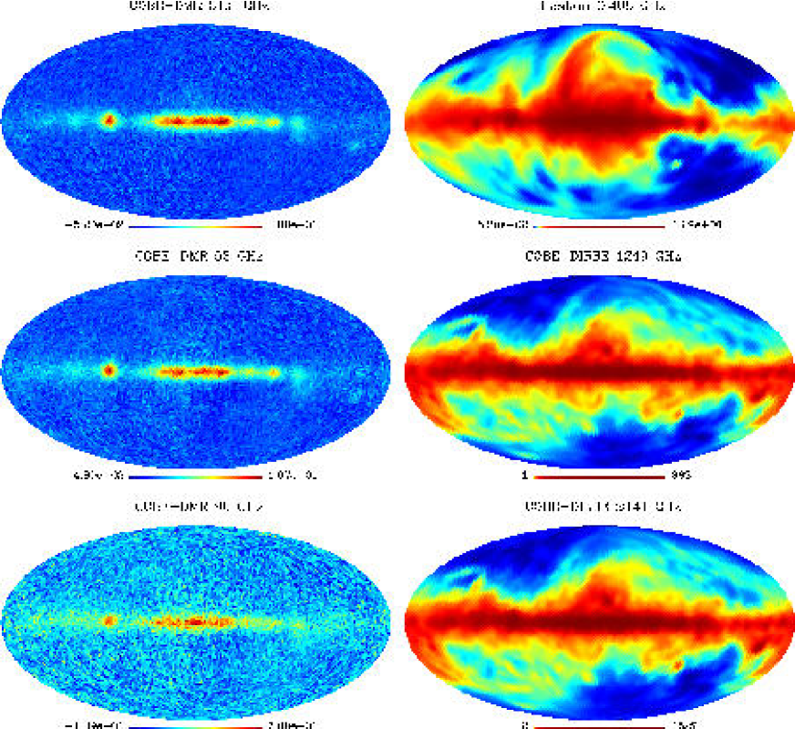
Figure 1: Data maps used in our analysis in units of MJy/sr. The left column shows the three COBE-DMR channels (from top to bottom): 31.5, 53 and 90 GHz. The top right panel gives the Haslam map and the middle and bottom right panels correspond to two of the COBE-DIRBE channels (1249 and 2141 GHz). The Haslam and COBE-DIRBE maps have been plotted in a non-linear scale to allow the visualization of the structure of the maps outside the galactic centre

A different approach is to run MEM for different sets of spectral parameters and try to infer from the reconstructed components which parameters give the best results and are, therefore, closest to the truth. One could naively look at the estimated errors and pick the reconstructions with the lowest values for these errors. However, the estimation of the errors depend on the chosen spectral parameters. Basically, it gives the statistical error of the reconstruction but it does not take into account uncertainties in the values of the spectral parameters. Therefore, if our guess of the frequency dependence is incorrect, the error estimation of the reconstructions is not reliable. Jones et al. (2000) showed that the dust frequency dependence could be estimated from Planck simulated data of small patches of the sky by minimising the $\chi^{2}$ of the reconstructions. They assumed a (spatially constant) grey body law for the dust emission with two unknown parameters (the dust temperature and emissivity), which they were able to fit from the data by looking at the minimum of the $\chi^{2}$ of the reconstructions. However, varying the spectral index $\beta$ of the synchrotron or free-free emissions (assuming a power law $I\propto\nu^{\beta}$) had little effect on the value of the $\chi^{2}$ and could not be determined in this way. This was due to the fact that both the synchrotron and free-free emissions have a low amplitude with respect to the rest of the components in the considered region of the sky and therefore the data could not provide enough information to fit these two components. In this case, the reconstructions of these two emissions were lost, but those of the other components were little affected. This application shows that, depending on the characteristics of the data (sky coverage, resolution, signal-to-noise ratio, frequency coverage, etc.) we may not be able to estimate some of the spectral parameters using just the $\chi^{2}$ value. Therefore, in order to estimate all the spectral parameters we may need to use also information coming from other variables, such as the entropy or the cross correlations between the reconstructed CMB and the galactic components. We have used such an approach to determine empirically the best reconstructions, which is explained in detail in $\S\ref{rec:goodness}$.

3 Spherical microwave datasets

The only spherical CMB dataset available during the development of the flexible MEM algorithm was COBE-DMR data. In order to enable the reconstruction of different components of emission, we also make use of the COBE-DIRBE and Haslam maps. Each of these maps exist in the HEALPix pixelization (Górski et al. 1999) with $N_{\rm side}=32$, which corresponds to 12288 pixels of size 107 arcminutes. Since each of these datasets has been described in detail elsewhere, we just give a brief description in this section. The data maps in MJy/sr are shown in Fig. 1.

The COBE-DMR data consists of three frequency maps: 31.5, 53 and 90 GHz (each of them obtained by the combination of two channels) with a resolution of $\sim 7$ degrees and a signal-to-noise ratio of around 2 per 10 degree patch. The COBE-DMR data have an anisotropic noise pattern that can be easily taken into account with our method. As an illustration we show the noise dispersion per pixel for the 53 GHz channel in Fig 2. The COBE beam is well characterized by the curve given in Fig. 3 (Wright et al. 1994). For comparison, a Gaussian beam with 7 degree of full width half maximum (FWHM) is also shown.

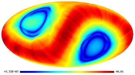
Figure 2: Dispersion noise per pixel of the COBE-DMR 53 GHz map in MJy/sr.

Figure 3: Window function of the COBE-DMR instrument (solid line). For comparison a Gaussian beam of FWHM=7^∘ is also shown (dotted line).

The COBE-DIRBE experiment observed the brightness of the full sky at ten wavelengths from 1.2 to 240 microns as well as mapping linear polarization at 1.2, 2.2 and 3.5 microns. In our analyses below we use the data at the two lowest frequencies (1249 and 2141 GHz). The maps have been degraded down to $N_{side}=32$ and smoothed with a Gaussian beam of FWHM 2.4 times the pixel size (i.e., FWHM =263.8 arcmin). The COBE-DIRBE noise is also anisotropic, but since we have significantly degraded the resolution of the data, its level is very small. The COBE-DIRBE beam has a resolution of 0.7 degrees and can be approximately modelled by a top-hat. At these frequencies, (thermal) dust emission dominates and therefore these data help the algorithm to extract the dust component.

The Haslam map gives the emission of the whole sky at 408 MHz and has been obtained by combining four different surveys (Haslam et al. 1982). It has an effective resolution of 51 arcminutes. Recently, Finkbeiner, Davis & Schlegel (private communication) have reprocessed the original Haslam map to provide a destriped, point-source subtracted map, which we have used for our analysis. We have degraded its resolution down to the HEALPix resolution of $N_{side}=32$ and smoothed it with a Gaussian beam of FWHM=263.8 arcmin. At this frequency the emission is dominated by galactic synchrotron, providing MEM with excellent information to trace this component.

4 Analysis of simulated data

Before applying of our flexible MEM component separation method to real data, we have checked its performance on simulated datasets. In order to simulate our sets of data (COBE-DMR, COBE-DIRBE and Haslam maps) we have assumed that the sky contains, CMB, free-free, synchrotron and thermal dust emissions. The four simulated maps at the reference frequency of 50 GHz are given in Fig. 4 in units of $\mu$K (thermodynamical temperature).

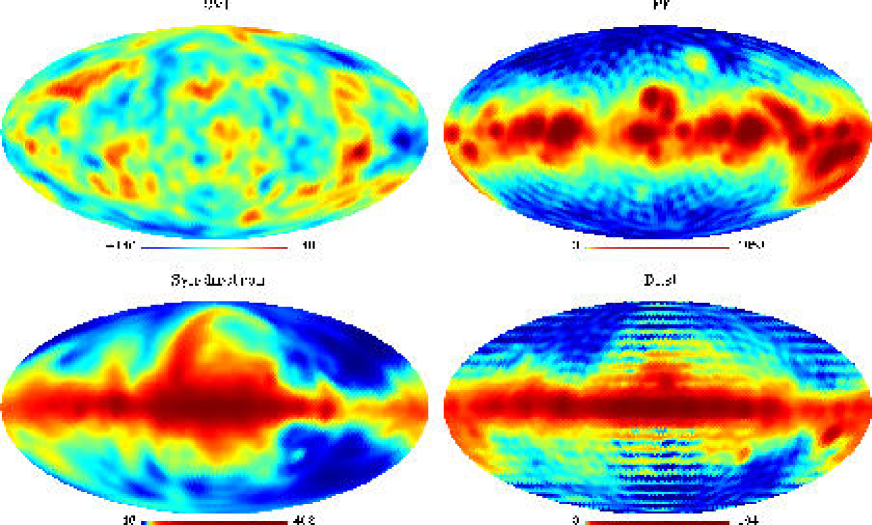
Figure 4: Input simulated components (from left to right and top to bottom): CMB, free-free, Synchrotron and dust at 50 GHz in $\mu$K (thermodynamical temperature). The maps have been smoothed with a 7 degree Gaussian beam. The galactic components have been plotted in a non-linear scale to allow for a better visualization of the high-galactic latitude region. To allow for a straightforward comparison with the reconstructed map, the input components include only information up to $\ell=40$. This produces the ringing artifacts visible in the dust map.

4.1 The simulations

The CMB realization has been produced with the help of the HEALPix package and has been constrained to have a power spectra compatible to the one derived from the COBE-DMR data (Bennett et al. 1996) at low $\ell$’s and from Archeops (Benoit et al. 2003) for higher multipoles. The synchrotron emission has been modelled by a power law $I_{\rm syn}\propto\nu^{-0.8}$ and the template at the reference frequency has been obtained by extrapolating the Haslam map with this law. The dust emission has been obtained by extrapolating the IRAS-DIRBE map of Schlegel, Finkbeiner & Davis (1998) using a single grey body component with dust emissivity of 2 and temperature of 18 K. Finally, the free-free component has been modelled with a power law of $I_{\rm ff}\propto\nu^{-0.16}$. As template for the free-free we have used the WHAM survey (Reynolds, Haffner & Madsen 2002), which provides an H_α map of most of the sky. The empty part of the sky has been filled in by copying on it another region of the survey. The map has been normalized to have a dispersion of 185 $\mu$K at 50 GHz and smoothed with a 7 degree Gaussian beam. This is several times higher than expected using estimations from the H_α emission (e.g. Finkbeiner 2003), but it is intended to account for the excess of emission found in the data whose origin is uncertain.

Table 1: Assumed observational parameters for the simulated data

	Haslam	DMR			DIRBE
Freq (GHz)	0.408	31.5	53	90	1249	2141
Resolution (∘)	4.5	$\sim$ 7	$\sim$ 7	$\sim$ 7	4.4	4.4
$\Delta\nu/\nu$	0.04	0.07	0.04	0.05	0.28	0.40

The separate components have been combined in order to simulate data according to the characteristics given in Table 1. For the COBE-DMR data we have used the true beam shape given in Fig. 3 and added Gaussian pixel noise according with the anisotropic pattern of the maps. Since we aim to reconstruct only four components (and in particular a single dust component) we have simulated only the lowest frequency COBE-DIRBE channel. We have ignored the beam of this experiment since it is small in relation to the pixel (and the subsequent smoothing). We have added the corresponding anisotropic noise at the COBE-DIRBE map. Signal plus noise have then been smoothed with a Gaussian beam of 263.8 arcmin. Finally, since the real Haslam map has been produced combining different surveys and has been degraded and reprocessed, it is not straightforward to determine the level of pixel noise present in the map, which will also be correlated. However, we expect it to be very small for the considered scales. Therefore, we have neglected the noise when generating the map, which has been simulated with an effective resolution of 268.7 arcminutes (51 arcminutes beam coming from the resolution of the Haslam map plus a smoothing of FWHM=263.8 arcminutes).

4.2 Results

We have applied the method explained in $\S\ref{sec:method}$ to our simulated data in order to recover the CMB and galactic foregrounds. Given the resolution and signal to noise of the data, we have aimed to reconstruct the different components only up to $\ell_{max}=40$, since there is virtually no information about the CMB in the data at higher multipoles. We need to provide the algorithm with an initial guess for the power spectra for each of the components. As shown in H98, the reconstructions are not very sensitive to this initial guess, provided one iterates over the power spectra, i.e. one performs the reconstruction with an initial guess and uses those reconstructed maps to provide starting power spectra for the next iteration, until convergence is obtained. For the galactic components, we have chosen initial power spectra that differ appreciably from the original input maps to show the performance of the method even when the initial power spectra are far from the correct ones. Regarding the CMB, we have chosen not to iterate over its power spectrum, but to start each iteration with a CMB model which is compatible (but that differs from the input one) with the power spectra derived from the COBE data (at the lowest $\ell$’s) and from Archeops (at the highest multipoles). As shown in S02, an approximated initial guess is enough for MEM to find the underlying power spectra. It must also be pointed out that if we were using a prior for the CMB power spectrum that significantly differs from the true one and we do not iterate over this quantity, this could bias the results obtained by the method, especially at those scales with a low signal to noise ratio. However, we do have a good knowledge of the shape of the power spectrum of the CMB at these low $\ell$’s. Therefore it is reasonable to make use of these information in order to improve the CMB reconstruction. In any case, we would like to emphasize that the knowledge of the CMB (or any of the other components) power spectrum is not necessary for the method to work. If there was a total absence of knowledge of the CMB prior, we would need to iterate over its power spectrum to find the correct reconstruction. In fact, if we were using high quality data, such an analysis without providing any prior information should also be performed. This would avoid biasing the results as well as point out possible inconsistencies with the supplied prior.

We also need an estimation of the noise for each data map. The noise of the COBE maps is well known, but this is not the case for the Haslam map, as mentioned in the previous section. In order to provide a reasonable value for the calculation of the $\chi^{2}$ function we have used the following trick. The Haslam map has some structure beyond $\ell=40$, but we are going to reconstruct the map only up to that multipole. Since the map has been smoothed and processed we expect the noise to be very small at the scales that we are reconstructing. Therefore when subtracting our predicted data map (generated using the reconstructions up to $\ell_{max}$) from the true data map to obtain the $\chi^{2}$, the difference will come mainly from the power beyond the maximum reconstructed multipole and that can be considered our effective noise. Therefore, the estimation of the noise for this simulated data map has been obtained as the dispersion of the map obtained subtracting the simulated Haslam map with power up to $\ell_{max}$ from the same map at full resolution. In practice we have used the same trick to estimate the noise of the COBE-DIRBE channel. This is due to the fact that the noise per pixel of this map is very low after repixelisation and smoothing and it was necessary to take into account the structure present beyond $\ell_{max}$, which was giving the main contribution to the $\chi^{2}$. This estimation of the noise produced $\chi^{2}$ in the correct range.

4.2.1 Estimation of the spectral parameters in a low noise case

Unfortunately the COBE-DMR data maps are very noisy, so it is difficult to test the performance of our method and, in particular, the determination of the spectral parameters, with this data set. Therefore, we have first tested our flexible MEM algorithm in an artificially low noise case. For this test, we have used the same simulations described in the previous section but the noise level of the COBE-DMR channels has been lowered by a factor of 5.

We have applied our method to this simulated data assuming different sets of spectral parameters. In particular, we have used all the possible combinations (a total of 81) of the following values: $\beta_{\rm ff}$=-0.13,-0.16,-0.19, $\beta_{syn}=-0.7,-0.8,-0.9$, $T_{\rm d}$=16,18,20 and $\alpha_{\rm d}$=1.8,2.0,2.2. For each set of spectral parameters we have iterated over the power spectra for all the galactic components to find the best possible reconstructions in each case. We have then looked at the $\chi^{2}$ value of the reconstructed maps for each combination of spectral parameters as an indicator of the quality of the reconstructions. We find that, as one would expect in an ideal case, the reconstruction with the lowest $\chi^{2}$ value (or equivalently $\chi^{2}/n_{f}$) corresponds to the one obtained using the correct set of spectral paramaters (i.e., $\beta_{\rm ff}$=-0.16, $\beta_{syn}=-0.8$, $T_{\rm d}$=18 and $\alpha_{\rm d}$=2.0). Since the noise of each data map is quite small, there is no room for uncertainties in the spectral indices and the $\chi^{2}$ successfully picks the right set of spectral parameters. We have numbered the different cases according to the obtained $\chi^{2}$ value. Case number 1 corresponds to the lowest $\chi^{2}$ whereas case 81 is the one with the highest $\chi^{2}$ value. Table 2 gives the value of the spectral parameters and of $\chi^{2}/n_{f}$ for the 10 first cases.

Table 2: Spectral parameters and value of $\chi^{2}/n_{f}$ for the ten best cases from low noise simulated data

Case	$T_{d}$	$\alpha_{d}$	$\beta_{ff}$	$\beta_{syn}$	$\chi^{2}/n_{f}$
1	18	2.0	$-0.16$	$-0.8$	12156
2	18	2.0	$-0.19$	$-0.8$	12167
3	18	2.0	$-0.13$	$-0.8$	12171
4	18	2.0	$-0.19$	$-0.9$	12215
5	16	2.2	$-0.13$	$-0.8$	12229
6	16	2.2	$-0.16$	$-0.8$	12237
7	16	2.2	$-0.19$	$-0.9$	12240
8	18	2.0	$-0.16$	$-0.9$	12244
9	20	2.0	$-0.13$	$-0.8$	12252
10	20	2.0	$-0.16$	$-0.8$	12258

In addition to the $\chi^{2}$ there are other quantities that can be calculated from the reconstructed components that also provide information about the quality of the reconstructions. In particular, we have also studied the behaviour of $\varphi/n_{f}$, $S/n_{c}$, the cross-correlations between the CMB reconstructed map and the three galactic components (which should be zero) and the dispersion of the CMB reconstructed map $\sigma^{\rm rec}_{\rm CMB}$. All these quantities are plotted in Fig. 5 versus the case number. The error $e_{\rm true}$ in the CMB reconstruction (smoothed with a 7 degree beam) is also shown and has been calculated as

$$e_{\rm true}=\sqrt{\langle(T_{i}-T_{r})^{2}\rangle-\langle T_{i}-T_{r}\rangle^{2}}$$ (15)

where $T_{i}$ and $T_{r}$ correspond to the input and reconstructed map smoothed with a 7 degree beam. It is interesting to note the high correlation between the value of the $\chi^{2}$ and the CMB reconstruction error. Moreover, this error correlates also very strongly with the rest of the plotted quantities. As one would expect, the maps with a low $e_{\rm true}$ also present values of the cross-correlations between the CMB and the galactic restored maps close to zero. Small values of $\varphi$ and $|S|$ correspond as well to small values of $e_{\rm true}$. Finally, we also find that the lowest values of $\sigma^{\rm rec}_{\rm CMB}$ are also the ones with better CMB reconstructions. This can be explained taking into account that those CMB recostructions obtained with wrong spectral indices will be contaminated by galactic emission and therefore the dispersion of the CMB map will increase.

Figure 5: The following quantities have been plotted versus the case number for the low-noise simulated case: left column (from top to bottom): $\varphi/n_{f}$, $\chi^{2}/n_{f}$, $S/n_{c}$ and dispersion of the reconstructed CMB map. Right column (from top to bottom): cross correlations between the reconstructed maps of CMB and free-free, CMB and synchrotron, CMB and dust and error of the CMB reconstruction. For reference, the dotted line in the cross correlation panels show the level of the correlation between the input maps of the CMB and the corresponding galactic component.

Since the main objective of this test was to study the estimation of the spectral parameters using different indicators of the quality of the reconstructions, we will not go into detail with regard to the reconstructed maps and power spectra. However we give, as reference, the difference reconstructed errors for the four recovered components in Table 3 for case 1.

Table 3: Dispersion values for input, reconstructed (from case 1) and residuals maps smoothed with a 7 degree beam at 50 GHz in $\mu$K for the low noise simulated data. These values are given for the whole map (col. 3) , for the region outside the galactic cut (col. 4) and for the galactic centre (col. 5). For comparison the estimated error is also given in the last column.

Cpt	Map	$\sigma_{all}$	$\sigma_{out}$	$\sigma_{Gal}$	$e_{est}$
	Input	36.4	36.5	36.3
CMB	Rec.	35.8	35.4	36.5
	Resid.	9.5	9.4	9.8	10.9
	Input	186.2	34.8	255.6
FF	Rec.	186.6	36.5	256.2
	Resid.	11.9	11.8	11.9	23.7
	Input	42.7	10.1	59.2
Synch.	Rec.	42.7	10.1	59.2
	Resid.	0.55	0.54	0.55	1.4
	Input	16.6	0.66	25.1
Dust	Rec.	16.6	0.66	25.1
	Resid.	0.08	0.08	0.08	1.3

4.2.2 Estimation of the spectral parameters in the simulated case with realistic noise

Figure 6: The panels show, for the realistic simulated data, the residuals dispersion (solid line) versus the case number for each of the reconstructed components after smoothing with a 7 degree Gaussian beam. For comparison the estimated error is also plotted (dashed line)

Figure 7: The quantities used to calculate $G$, and $G$ itself, are plotted versus the case number for the simulations. Left column (from top to bottom): $\varphi/n_{f}$, $\chi^{2}/n_{f}$, $S/n_{c}$ and dispersion of the reconstructed CMB map. Right column (from top to bottom): cross correlations between the reconstructed maps of CMB and free-free, CMB and synchrotron, CMB and dust and $G$. For reference, the dotted line in the cross correlation panels show the level of the correlation between the input maps of the CMB and the corresponding galactic component.

Figure 8: Spectral parameters versus case number for the simulations: dust model (top), spectral index for the free-free (middle) and spectral index for synchrotron (bottom). The dust model number correspond to: $T_{d}$=18,$\alpha_{d}$=2 (1), $T_{d}$=20,$\alpha_{d}$=1.8 (2), $T_{d}$=16,$\alpha_{d}$=2 (3), $T_{d}$=16,$\alpha_{d}$=2.2 (4), $T_{d}$=20,$\alpha_{d}$=2 (5), $T_{d}$=18,$\alpha_{d}$=2.2 (6), $T_{d}$=20,$\alpha_{d}$=2.2 (7), $T_{d}$=18,$\alpha_{d}$=1.8 (8), $T_{d}$=16,$\alpha_{d}$=1.8 (9).

We have repeated the previous analysis using our (realistic) simulated data set and have obtained reconstructions for the same 81 combinations of spectral parameters. As in the previous case the reconstructions have been obtained iterating over the power spectra of the galactic components for each set of spectral parameters. We have then investigated the behaviour of the different quantities that might indicate which combination of parameters is correct. If we look at the reconstruction with the lowest $\chi^{2}$ value we find the following set of parameters: $T_{d}=18$, $\alpha_{d}=2.0$, $\beta_{\rm ff}=-0.13$, $\beta_{\rm syn}=-0.7$ (corresponding to a $\chi^{2}/n_{f}=12191$) whereas the reconstruction with the correct spectral parameters has the second lowest $\chi^{2}$ value which is also very close to the minimum ($\chi^{2}/n_{f}=12192$). In fact, 3 more of the reconstructions have values $\chi^{2}/n_{f}<12193$. Therefore we find that the data are just too noisy to discriminate clearly between different spectral data sets using just the information given by the $\chi^{2}$. However, we have seen in the previous section that there is more information that we can extract from the reconstructed maps to assess the quality of the reconstructions and to determine the spectral parameters. Therefore, we have also considered the values of the entropy $S$, the $\varphi$ function, the dispersion of the reconstructed CMB map $\sigma_{\rm CMB}^{\rm rec}$, and the cross-correlation between the reconstructed CMB and each of the reconstructed galactic components. In particular we have constructed an empirical selection function $G$ that is a linear combination of the former quantities and is defined as

$$G = \frac{1}{\sum_{i}a_{i}}\left[a_{1}\frac{\chi^{2}}{n_{f}}+a_{2}\frac{\varphi}{n_{f}}+a_{3}\frac{|S|}{n_{c}}+a_{4}|c_{\rm ff}|\right.$$ (16)

$$\hskip 28.45274pt\left.\phantom{\frac{\chi^{2}}{n_{f}}}+a_{5}|c_{\rm syn}|+a_{6}|c_{\rm dust}|+a_{7}\sigma_{\rm CMB}^{\rm rec}\right],$$

where $c_{j}$ denotes the cross-correlation between the CMB reconstruction and the corresponding galactic component. The minimum of $G$ will give us the best reconstructions. The chosen weights $a_{i}$ are given in Table 4 and have been determined by looking for an optimal combination that gives more weight to those reconstructions with higher quality and whose spectral parameters deviate less from the true ones. The goal of combining all this information is that even if we can not reliably determine the spectral parameters, given the low signal to noise of the data, at least we can prevent the uncertainties in the knowledge of such parameters from severely contaminating the CMB reconstruction.

Table 4: Weights for the calculation of $G$

Coefficient	Value
$a_{1}$	0.6
$a_{2}$	0.6
$a_{3}$	5
$a_{4}$	100
$a_{5}$	100
$a_{6}$	100
$a_{7}$	1

Table 5: Spectral parameters and value of $G$ for the ten best cases from (realistic) simulated data

Case	$T_{d}$	$\alpha_{d}$	$\beta_{ff}$	$\beta_{syn}$	$G$
1	18	2.0	$-0.16$	$-0.8$	54.0050
2	18	2.0	$-0.19$	$-0.9$	54.0055
3	18	2.0	$-0.13$	$-0.8$	54.0063
4	18	2.0	$-0.19$	$-0.8$	54.0084
5	18	2.0	$-0.16$	$-0.9$	54.0085
6	20	1.8	$-0.19$	$-0.7$	54.0525
7	18	2.0	$-0.13$	$-0.9$	54.0536
8	16	2.0	$-0.19$	$-0.7$	54.0547
9	18	2.0	$-0.16$	$-0.7$	54.0556
10	18	2.0	$-0.13$	$-0.7$	54.0563

Using $G$, we find that the preferred reconstruction is the one with the correct spectral paramaters, whereas that with the lowest $\chi^{2}$ value is now in position 10 (see Table 5 to see the values of the parameters for the first 10 cases). The different cases have been ordered according to the value of $G$, so those cases with a lower number correspond to sets of parameters that produce a smaller $G$. It is interesting to note that the smoothed 7 degree CMB reconstruction error of the case prefered by the $G$ quantity (case 1) is $21.5\mu$K whereas that of the case with the minimum $\chi^{2}$ (case 10) is $22.9\mu$K. In fact if we calculate the correlation between the values of $G$ and of the CMB reconstructed error for the 81 cases we find a value of 0.993 versus 0.969 for the correlation between the $\chi^{2}$ value and the same error. In addition, there is also another importan reason to use the combined information rather than just the $\chi^{2}$. For real data, where the foregrounds can not be well modelled by a simple law, or where systematics may be present, it seems a good idea to combine all the available information. In particular, the $\chi^{2}$ will not perform as well as in the ideal case and therefore we should also make use of quantities such as the cross-correlations between CMB and the galactic components that can be more reliable to assess the quality of the reconstruction for real data.

The behaviour of the quantities used to construct $G$ is illustrated in Figs. 6,  7 and  8. The different quantities have been plotted versus the case number (ordered according to $G$); Fig. 6 shows the dispersion of the residuals (solid line) for each of the components smoothed with a 7 degrees Gaussian beam. Note that in the CMB case, there is a clear correlation between the reconstruction error and the ordering of the cases: a lower value of $G$ (which is plotted in the bottom right panel of Fig. 7) will produce in general a better CMB reconstruction. It is also striking that this error varies very little for the cases with the lowest values of $G$ In fact, the difference outside the galactic cut between the CMB reconstruction (smoothed with a 7 degree Gaussian beam) of case 1 and all those up to case 25 is $\leqslant 3\mu$K, which is well below the statistical errors. As expected, the CMB reconstruction in the galactic region is more dependent on the spectral parameters and the differences range between $3-12\mu$K for the same cases. The dashed lines in Fig. 6 indicate the residuals dispersion estimated by our method. As already mentioned, this error is only reliable if the spectral parameters are close to the true values. If this is the case, this error gives a good estimation of the residuals dispersion.

Fig. 7 shows some additional sensitive quantities versus the case ordering. We see that low values of $\chi^{2}$, $\varphi$ and of the absolute value of the entropy also go in the direction of producing better reconstructions. In addition, the cross correlations between the reconstructed CMB and galactic components are also indicators of the reliability of the reconstructions. Another very interesting result is given in the bottom left panel of Fig. 7, where the dispersion of the reconstructed CMB map smoothed with a 7 degree Gaussian beam is given. The correlation between this quantity and the actual error of the CMB map is striking. As already mentioned, this can be understood since errors in the CMB restored map would mainly come from the introduction in the reconstruction of galactic contamination, which will give rise to a higher dispersion of the map. The fact that different foreground models produce similar CMB reconstructions indicate that we have degenerate cases, due again to the low signal-to-noise ratio of our data.

This effect can be seen in the two bottom panels of Fig. 8, where the spectral indices for the free-free and synchrotron are plotted versus the case number. There is no clear trend between these parameters and the quality of the reconstruction. Therefore, these data are not precise enough to determine unambiguously the free-free and synchrotron parameters. However, it is still important to look at all the available information, since not all combinations of $\beta_{\rm ff}$ and $\beta_{\rm syn}$ produce equally good CMB reconstructions. In the case of the dust component (see bottom right panel of Fig. 6 and top panel of Fig. 8) there is a visible correlation between the correct dust model and the case ordering. Therefore the dust parameters can be determined by the method itself for the case of a spatially invariant dust model. In a real data set, where spectral variability would occur, the picture would not be so clear, but there would still be some trends in the graphs that would point out to some preferred models (see discussion in next section).

We note that there are other possible choices of weights that would assign the best $G$ to the case with the correct spectral parameters. In fact, in practice, it would be very difficult to distinguish between the five cases with a lower (and almost identical) value of $G$ for this data set, since other similar choices of weights lead to a reordering of the top cases. We remark, however, that the CMB reconstruction is very robust independently of the chosen spectral parameters for those cases with low values of $G$. The fact that $G$ is so flat indicates again that the data are too noisy to discriminate unambiguosly between the different sets of spectral parameters. MEM is able to accomodate a handful of different models within the noise, providing virtually indistinguishable CMB reconstructions.

Figure 9: Value of $G$ versus case number (ordered from low to high value of $\chi^{2}$) for the low noise case.

It is interesting to look at the result if we apply the selection function $G$ to the low noise simulated case of the previous section. Fig. 9 shows the values of the $G$ function versus the case number in the low noise case. Note that the cases are ordered according to the value of the $\chi^{2}$ obtained in the low noise reconstructions and therefore the numbering does not coincide with the one on this section. As expected, the $G$ selector works also in this case and the reconstruction with the minimum value of $G$ coincides with the one obtained with the minimum value of $\chi^{2}$ (which had the correct spectral parameters). The fact that the value of $G$ is higher for the low noise case with respect to the realistic case should not be surprising. $G$ can be used to compare different reconstructions for the same experiment. However it should not be used to compare the quality of reconstructions for experiments with different characteristics. For instance, MEM gives more weight to minimising the value of the $\chi^{2}$ than that of the entropy in the low noise case producing a higher value of S (although with a slightly lower value of $\alpha$) what contributes to a higher $G$. Also the value of $\sigma^{\rm rec}_{\rm CMB}$ is higher in the low noise case since the CMB has been reconstructed with (intrinsic) higher resolution. A more interesting conclusion can be derived by looking at the range of $G$ for the low and realistic noise cases. Whereas $G$ spans from $\sim 56$ to $\sim 73$ for the low noise case, in the realistic case the range for the same 81 cases goes from $\sim 54$ to $\sim 56$. This shows again that the low signal to noise of the realistic data make it very difficult to discriminate between the different considered cases. We also note that the optimal choice of the coefficients defining $G$ may vary depending on the characteristics of the considered experiment. Therefore, a detailed study using simulations should be performed in each case.

4.2.3 Reconstructed maps and power spectra for the simulated case with realistic noise

We have plotted the reconstructed maps corresponding to case 1 (i.e. using the correct spectral parameters) smoothed with a 7 degree Gaussian beam in Fig. 10 in the same scale as the input maps (Fig. 4) to allow for a straightforward comparison. The residuals map for each component is given in Fig. 11. The values of the residuals dispersion for each component (all-sky, high and low galactic latitude), the dispersion of the input maps and the estimated errors are summarized in Table 6.

Table 6: Dispersion values for input, reconstructed (from case 1) and residuals maps smoothed with a 7 degree beam at 50 GHz in $\mu$K. These values are given for the whole map (col. 3) , for the region outside the galactic cut (col. 4) and for the galactic centre (col. 5). For comparison the estimated error is also given in the last column.

Cpt	Map	$\sigma_{all}$	$\sigma_{out}$	$\sigma_{Gal}$	$e_{est}$
	Input	36.4	36.5	36.3
CMB	Rec.	34.3	33.2	37.4
	Resid.	21.5	21.4	21.3	21.8
	Input	186.2	34.8	255.6
FF	Rec.	187.2	46.9	256.3
	Resid.	36.9	33.2	42.4	42.0
	Input	42.7	10.1	59.2
Synch.	Rec.	42.8	10.2	59.4
	Resid.	1.7	1.5	1.9	2.1
	Input	16.6	0.66	25.1
Dust	Rec.	16.6	0.66	25.1
	Resid.	0.04	0.03	0.05	1.3

The dispersion of the CMB residuals on an angular scale of 7 degrees is at the level of $\sim 21$ $\mu$K, which is in good agreement with the estimated error given by the MEM algorithm (see Table 6). Many of the main features of the CMB input map are also present in the reconstruction. However, the smallest structure has clearly been damped in the reconstructed map. This is expected since at the highest considered $\ell$’s the COBE-DMR data are dominated by noise and MEM just defaults to zero in absence of any useful information. It is interesting to point out that the CMB errors at high and low galactic latitudes are actually comparable ($\sim 21\mu$K in both cases, see Table 6), showing that the map is equally well recovered independently of the Galaxy. This is the case even for small departures of the spectral parameters from the true ones, such as those in the 5 best cases, which have very similar residuals dispersions in both regions. This is due to the very high noise of the COBE-DMR maps that allows to accommodate the data to different spectral models. In fact, as already mentioned, the CMB reconstruction is very robust for models with a low value of $G$. The difference between the 7 degree smoothed CMB reconstruction of case 1 and those of cases 2 to 5 are $<2\mu K$ outside the Galaxy and $<4\mu K$ inside the galactic cut for all the cases, values which are significantly lower than the statiscal error. Therefore, even if we can not determine with total reliability the spectral parameters from our data set due to their low signal-to-noise, we can avoid the introduction of errors in the CMB reconstruction due to these uncertainties, especially at the high galactic latitude region. For cases with larger values of $G$, the reconstructed error inside the Galaxy starts to be systematically higher than that of the high galactic latitude region.

Regarding the free-free map, it can be seen that the galactic plane is reasonably well recovered (with an error $\sim$20 per cent) whereas most of the structure outside the galactic cut has been lost. In fact much of the signal recovered at high galactic latitude takes negative values. The synchrotron and dust maps have been very well recovered since MEM has succeeded in tracing these emissions from the Haslam and COBE-DIRBE maps respectively. There are only some small differences between the input and reconstructed maps, mostly at small scales, and the dispersions of the residuals are at the level of $\sim 4$ per cent for the synchrotron and $\sim 0.3$ per cent for the dust component.

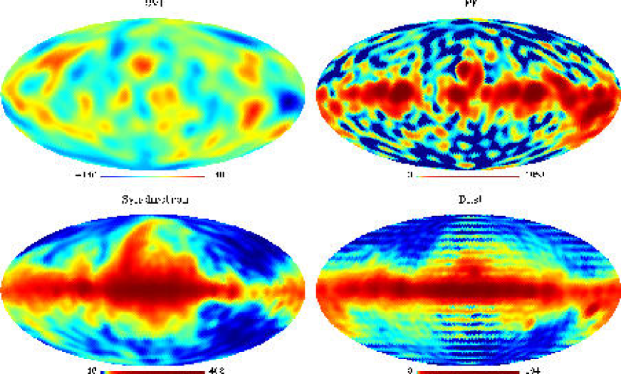
Figure 10: Reconstructed components from realistic simulated data at 50 GHz obtained using the correct spectral parameters (case 1). The maps have been smoothed with a 7 degree Gaussian beam and have been plotted in the same scale as the input maps of Fig. 4 to allow a straightforward comparison

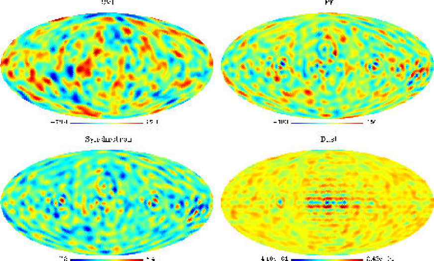
Figure 11: Residuals of the simulated data for the correct spectral parameters (case 1) obtained by subtracting the smoothed input maps (Fig. 4) from the smoothed reconstructions (Fig. 10). All the maps have been plotted in linear scale.

Of course, when the wrong spectral dependence is assumed, the errors increase appreciably for all the galactic components. However, these differences come mainly from a normalization factor rather than from the spatial structure. For instance the reconstruction error for the synchrotron in case 2 (where $\beta_{syn}=-0.9$ was assumed) is $\sim 17\mu$K (versus $\sim 2\mu$K for case 1) whereas the spatial cross correlation between the input and reconstructed smoothed maps is at the same level (0.999) for both cases. Thus, MEM is finding the right amplitude and structure of the synchrotron at the Haslam frequency, where this emission dominates, and then extrapolating to the reference frequency using the considered spectral index. Similar ideas apply to the dust and free-free emissions.

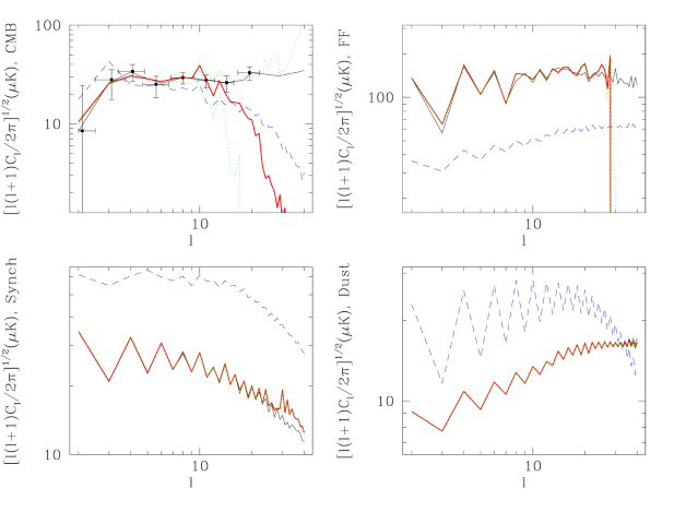
Figure 12: Original (thin solid), initial guess (dashed) and reconstructed (thick solid) power spectra for the (realistic) simulated data. The dotted lines indicate the estimated 1$\sigma$ confidence level for the reconstructed power spectra. The correct spectral parameters have been used for the reconstructions (case 1). For comparison the power spectra measurements obtained from the COBE-DMR data are also shown (solid squares in top left panel, taken from Tegmark & Hamilton 1997).

In Fig. 12 the true (thin solid line) and reconstructed (thick solid line) power spectra for the unsmoothed input and recovered maps have been plotted. The dotted lines are the estimated $1\sigma$ confidence level for the reconstructed components. Finally, the dashed line correspond to the initial power spectra supplied to the MEM algorithm. In the CMB panel (top right) we have also plotted the power spectra measured from COBE (solid squares). Note that the CMB power spectrum used as initial guess in MEM (dashed line) is similar but differs from the true one (thin line), allowing for possible errors in the estimation of the prior. Even without iterating in the CMB power spectra, the recovered $C_{\ell}$’s follow quite well the true ones up to $\ell\sim 15$ and then start to drop due to the resolution of the COBE-DMR data. As already mentioned, this reflects a loss of resolution in the reconstructed map with respect to the input one. We may also wonder about the quality of the recovered power spectra inside and outside the galactic cut. Fig. 13 shows the true and reconstructed power spectra in these two regions of the sky. For simplicity, we have estimated the $C_{\ell}$’s padding with zeros the masked region and they have been rescaled according to the considered area. For the CMB case the results are quite similar for both regions of the sky, and the reconstructed power spectrum follows approximately the true power up to $\ell\sim 15$, as it was the case for the whole sky.

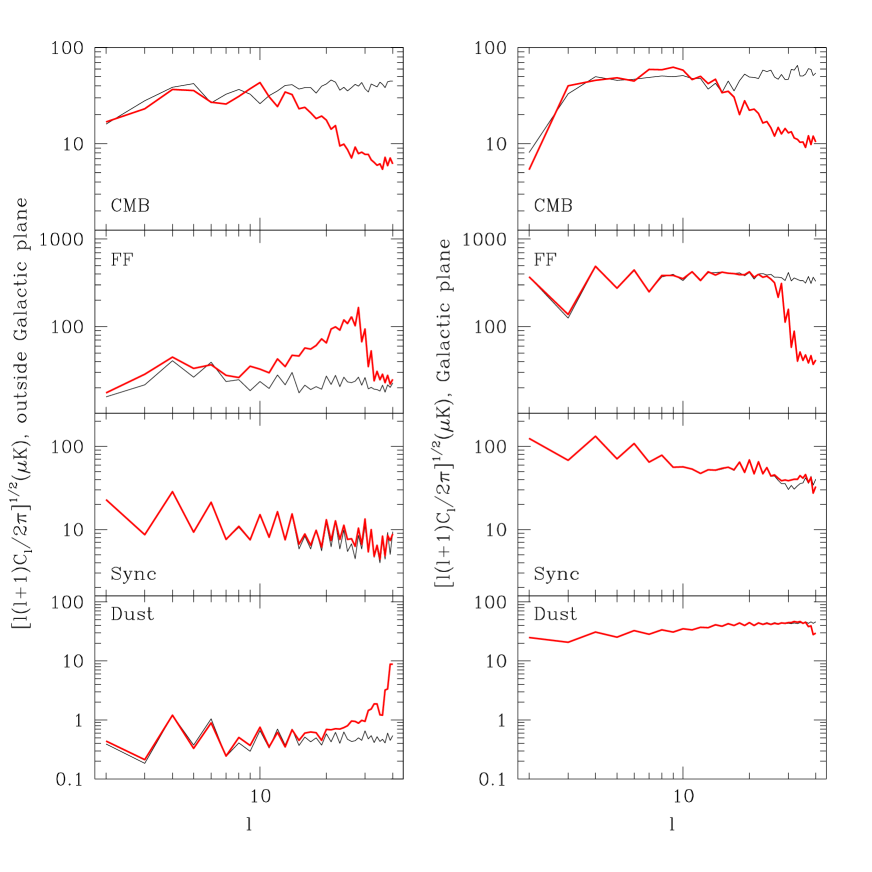
Figure 13: Original (thin solid) and reconstructed (thick solid) power spectra for the simulated data inside and outside the galactic plane. The correct spectral parameters have been used for the reconstructions (case 1).

Regarding the galactic components, it is quite striking that MEM is able to recover the right power spectra even when the initial guess was far off from the correct $C_{\ell}$’s. The free-free power spectra (top right panel of Fig. 12) has been reasonably well recovered up to $\ell\sim 30$ (although some excess is present at the smallest scales) where it sharply drops to zero. As in the case of the CMB, the free-free information comes mainly from the noisy COBE-DMR data whose signal to noise ratio and resolution does not allow MEM to provide a reconstruction at higher $\ell$’s. An interesting result is also found by looking at Fig. 13. The reconstructed FF power spectrum inside the galactic plane follows quite well the input one up to $\ell\sim 25$, however the reconstruction is much poorer outside the galactic cut. In fact, a clear excess of power is seen at $\ell\ga 10$, which gives rise to the spurious structure that is present in the FF reconstructed map at high galactic latitude and to the excess of power seen in the whole-sky reconstructed power spectrum. The reason for MEM to fail in recovering the FF in this region of the sky is again the low signal-to-noise ratio of the data together with the weakness of the FF component outside the Galaxy. The synchrotron is faithfully recovered up to $\ell\ga 20$, result that holds for both the high and low galactic latitude regions as well as for the whole map reconstruction. At higher $\ell$’s there is some excess power which is responsible for the structure seen in the synchrotron residuals. Finally, the recovered dust power spectra in the galactic region follows very well the input one up to practically the considered $\ell_{max}$. This is due to the fact that the dust emission is mainly recovered from the COBE-DIRBE map, which provides the algorithm with enough resolution to recover faithfully this component up to very high $\ell$. Regarding the high galactic latitude region, there is an excess of power present at $\ell\ga 20$. However this structure does not show in the global power spectrum reconstruction, which is very good up to high $\ell$, since this is dominated by the emission at the galactic region, which has been very well recovered.

5 Analysis of real data

We have applied our MEM algorithm to the set of data described in $\S\ref{sec:data}$. As in the previous section, we have aimed to reconstruct the CMB, free-free, synchrotron and dust emissions using the COBE-DMR, Haslam and the lowest frequency COBE-DIRBE maps. As the initial guess for our reconstructions we have chosen the power spectra of the simulated components of the previous sections (smoothed with the COBE-DMR beam for the CMB and the free-free and with a Gaussian beam of $\mbox{FWHM}=263.8$ arcmin for the dust and synchrotron). As before, we have iterated over the power spectra for the galactic components but not for the CMB, since we have some prior knowledge about its power spectra that we would like to include in the analysis.

5.1 Estimation of the spectral parameters

First of all we have applied MEM for 180 different sets of spectral parameters with values in the range 16 to 22 K for the dust temperature, 1.6 to 2.2 for the dust emissivity, $-0.9$ to $-0.6$ for $\beta_{syn}$ and $-0.19$ to $-0.13$ for $\beta_{ff}$. We have then ordered the different cases according to the obtained value of $G$. The lowest value of $G$ is obtained for the parameters $T_{d}=19$ K, $\alpha_{d}=2$, $\beta_{ff}=-0.19$ and $\beta_{syn}=-0.8$. Fig. 14 shows the values of the spectral parameters versus the case number.

Figure 14: Dust model (top), free-free spectral index (middle) and synchrotron spectral index (bottom) versus the case number for real data. The dust model number correspond to: $T_{d}=19$,$\alpha_{d}=2$ (1), $T_{d}=18$,$\alpha_{d}=2$ (2), $T_{d}=16$,$\alpha_{d}=2.2$ (3),$T_{d}=22$,$\alpha_{d}=1.8$ (4), $T_{d}=20$,$\alpha_{d}=2$ (5),$T_{d}=16$,$\alpha_{d}=2$ (6),$T_{d}=20$,$\alpha_{d}=1.8$ (7), $T_{d}=19$,$\alpha_{d}=1.8$ (8),$T_{d}=22$,$\alpha_{d}=2$ (9),$T_{d}=18$,$\alpha_{d}=2.2$ (10), $T_{d}=18$,$\alpha_{d}=1.8$ (11),$T_{d}=20$,$\alpha_{d}=2.2$ (12),$T_{d}=19$,$\alpha_{d}=2.2$ (13),$T_{d}=22$,$\alpha_{d}=1.6$ (14), $T_{d}=16$,$\alpha_{d}=1.8$ (15),$T_{d}=20$,$\alpha_{d}=1.6$ (16), $T_{d}=18$,$\alpha_{d}=1.6$ (17),$T_{d}=16$,$\alpha_{d}=1.6$ (18)

In Fig. 15 the value of $G$ as well as the quantities used to calculate it are given for the 180 cases. It can be seen that the trends of the curves are the same as those of the simulated cases (compare with Fig. 7). Not surprisingly, the value of $\varphi$, $\chi^{2}$, $|S|$ and $\sigma_{CMB}^{rec}$ are now a bit higher than in the simulated case, which indicates that our model does not perfectly fit the data. This is due to the large number of uncertainties present in the real case, such as the spectral dependence of each component, its position and/or frequency variability or even the number of components. However, the $\chi^{2}$ is still very reasonable since it is of the order of the number of data. As in the case of the simulated data, there is a clear correlation between the dust model (top panel) and the value of $G$, indicating that some of the studied dust parameters are preferred by the data. In particular models with $\alpha_{d}=2$ and $T_{d}$ around 18-20 K are in the first positions. Conversely, the considered models with $\alpha_{d}=1.6$ are clearly disfavoured. As expected, the distinction between the models is less clear than for the simulated data, since degenerate cases are more important for true data than for ideal ones. Regarding the free-free spectral index (middle panel), there is a slight trend from the data to favour those cases with more negative values of $\beta_{ff}$. Values of $\beta_{syn}$ between $-0.9$ and $-0.7$ are basically equally preferred by the data, whereas $\beta_{syn}=-0.6$ seems to produce reconstructions with higher values of $G$. Finally, for comparison with the ideal simulated case, we have plotted the estimated error for the reconstructed components in Fig. 16. They are at similar levels as those in the simulated cases.

Table 7 gives the ten cases with the lowest values of $G$. The difference between the CMB reconstruction for the selected case one and all the cases up to number 15 is between 0.8 and 2.8 $\mu$K outside the galactic cut and between 1.6 and 10 $\mu$K in the galactic centre. Therefore, as happened in the ideal case, the CMB recovered map in the high galactic latitude region is very robust against certain variations of spectral parameters.

Table 7: Spectral parameters and value of $G$ for the ten best cases from real data

Case	$T_{d}$	$\alpha_{d}$	$\beta_{ff}$	$\beta_{syn}$	$G$
1	19	2.0	$-0.19$	$-0.8$	54.6674
2	18	2.0	$-0.19$	$-0.8$	54.6678
3	18	2.0	$-0.19$	$-0.7$	54.6747
4	16	2.2	$-0.19$	$-0.9$	54.6812
5	22	1.8	$-0.19$	$-0.7$	54.6933
6	20	2.0	$-0.19$	$-0.9$	54.6946
7	18	2.0	$-0.19$	$-0.9$	54.7056
8	19	2.0	$-0.16$	$-0.8$	54.7216
9	18	2.0	$-0.16$	$-0.7$	54.7223
10	22	1.8	$-0.19$	$-0.8$	54.7227

Figure 15: As Fig. 7 but for the 180 cases used to recover the microwave sky from the real data.

Figure 16: Estimated errors of each of the reconstructed components versus the case number for the real data. Each case corresponds to a different set of spectral parameters and they have been ordered according to the value of $G$.

5.2 Reconstructed maps and power spectra

Fig. 17 shows the reconstructed CMB, free-free, Synchrotron and dust emissions for case 1 ($T_{d}=19$, $\alpha_{d}=2$, $\beta_{ff}=-0.19$ and $\beta_{syn}=-0.8$).

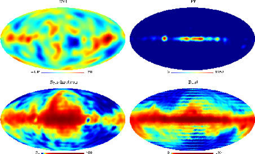
Figure 17: Recovered components smoothed with a 7 degree Gaussian beam from real data for the spectral parameters $T_{d}$=19 K, $\alpha=2$, $\beta_{ff}=-0.19$ and $\beta_{syn}=-0.8$ (case 1) at 50 GHz in $\mu$K. The synchrotron and dust components have been plotted in a non-linear scale.

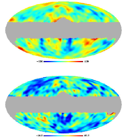
Figure 18: Top: coadded 53 and 90 GHz COBE-DMR maps smoothed with a 7 degree Gaussian beam in $\mu$K outside the galactic cut. The map is plotted in the same scale as the CMB reconstruction of Fig. 17. Bottom: the difference between the top map minus the CMB reconstructed map of Fig. 17 outside the galactic cut is shown. For the comparison, the monopole and dipole outside the galactic region have been subtracted from the coadded and reconstructed maps.

Table 8: Dispersion values for the reconstructed components from real data smoothed with a 7 degree Gaussian beam at 50 GHz in $\mu$K (for case 1) for the realistic simulated data. These values are given for the whole map (col.2), for the region outside the galactic cut (col.3) and for the galactic centre (col.4). The estimated error is also given in column 5.

Component	$\sigma_{all}$	$\sigma_{out}$	$\sigma_{Gal}$	$e_{est}$
CMB	41.1	35.0	47.4	21.8
FF	238.4	40.9	360.7	47.7
Synch.	33.6	10.7	45.6	2.6
Dust	12.6	0.67	18.6	0.88

Table 8 gives the dispersion level of the reconstructed components smoothed with a 7 degree Gaussian beam at the reference frequency of 50 GHz, for the whole-sky, the Galaxy and the high galactic latitude region. For the CMB, we can see that the dispersion for the two considered regions differ appreciably (35 versus 47 $\mu$K). This indicates that there is some contamination at low galactic latitudes in the CMB reconstructed map. This is not surprising given the uncertainties present in our model of the data (spatial variability of spectral parameters, frequency model for each component, number of present components, possible systematics, etc.). The estimated error of the CMB reconstruction on a scale of 7 degree is $\sim 22\mu$K. However, given the contamination of the CMB map in the galactic centre, we can consider that this value is a fair estimate of the CMB residuals only outside the galactic cut.

For comparison we have also plotted in Fig. 18 a CMB map obtained by coadding the 53 and 90 GHz COBE-DMR maps (each pixel weighted according to the inverse of its noise variance) which has been smoothed with a 7 degree Gaussian beam. To allow for a better comparison, we have removed the monopole and dipole outside the galactic cut which were mainly due to galactic emission. As expected, we find this map to be well correlated with our reconstructed CMB map (whose monopole and dipole have also been removed outside the galactic mask to calculate this correlation), at the level of 0.85 (outside the galactic cut), which confirms the presence of CMB signal in our reconstruction. The difference between this coadded map and our reconstruction outside the galactic cut is also shown in the same figure (bottom). Note the smaller scale range in the difference map which indicates the presence of common structure in both maps. However, some clear structure is also seen in the difference map. This is not surprising since not attempt to remove foreground emission has been made in the coadded map.

Regarding the free-free reconstructed map (top right panel of Fig. 17), we are able to recover emission only inside the galactic cut. As in the simulated case, the free-free signal at high galactic latitude is lost. In fact, the signal recovered outside the galactic cut takes mainly negative values and its dispersion is lower than the estimated error ($\sim 48~{}\mu$K). Regarding the galactic centre, MEM has only been able to recover emission in $\sim 30$ per cent of the area of the galactic cut, whereas the rest of the signal has zero or negative values. The dispersion level of the 7 degree smoothed free-free component in the galactic plane is $\sim 238\mu$K considering all pixels and it increases to $\sim 491\mu$K if we consider only the fraction of pixels with physical (i.e. positive) emission. This is several times higher than expected from current $H\alpha$ estimations and raises again the issue of an anomalous component. It is also interesting to note the high spatial correlation between the galactic plane of the reconstructed free-free map and that of the COBE-DMR frequency channels.

The synchrotron reconstructed map (bottom left panel of Fig. 17) presents structure both inside and outside the Galaxy. As expected, the reconstructed emission is very well correlated with the Haslam map (0.96 for the smoothed maps). We find a level of $\sim 46\mu$K for the synchrotron emission in the Galaxy and of $\sim 11\mu$K outside the Galaxy. The estimated error in the reconstruction is $2.6\mu$K. We should note, however, that this is the statistical error associated to our method but it does not take into account the uncertainties in the determination of $\beta_{\rm syn}$.

Finally, the bottom right panel of Fig. 17 shows the reconstructed dust emission smoothed with a 7 degree Gaussian beam. The visible ringing is an artifact due to the fact that we are recovering the dust only up to $\ell_{max}=40$, whereas the DIRBE data map (from which the algorithm traces this component) has power at higher multipoles. We have found a dispersion value for the dust component of $\sim 19\mu$K and of $\sim 0.7\mu$K inside and outside the Galaxy respectively at 50 GHz. The (statistical) estimated error is below 1 $\mu$K.

The (unsmoothed) reconstructed power spectra (solid line) for the four recovered components are given in Fig. 19. The dashed lines show our initial guess for the power spectra and the dotted lines indicate the 1$\sigma$ confidence level for the reconstructed power spectra. Fig. 20 shows the power spectra for the four reconstructed components inside and outside the galactic cut, that have been estimated in the same way as for the simulations.

For comparison we have also plotted the CMB measurements obtained for COBE-DMR in the CMB panel (top-left) of Fig. 19. It is interesting to note that the recovered $C_{\ell}$’s follow the shape of the power spectra measured from the COBE-DMR data but with a higher normalization. In addition, the reconstructed CMB power spectra for the high galactic latitude region (top left panel of Fig. 20) has approximately the expected amplitude whereas the one at the Galaxy (top right panel of Fig. 20) presents an excess of power at all scales. These are also indications of the fact that we have some galactic contamination in our reconstructed map, especially at high galactic latitudes.

The free-free reconstructed power spectra presents the same behaviour as in the simulated case. It seems to be recovered up to $\ell=30$ and then drops sharply to zero, due to the low resolution of the COBE-DMR channels, which MEM has mainly used to recover the free-free signal. We also find in the reconstructed power spectra inside and outside the Galaxy the same pattern as in the simulations. In particular, it seems to be an excess of power at large $\ell$ at high galactic latitude, which produces all the spurious signal that is found in this region of the FF reconstructed map.

The shape of the synchrotron reconstructed power spectra (bottom left panel) follows quite well that of the input one up to $\ell\sim 25$ but with a lower normalization. This is expected since the initial power spectra has been obtained from a smoothed extrapolation of the Haslam map up to the reference frequency using a spectral index of $-0.8$ (the same value as $\beta_{\rm syn}$ in our case). This extrapolation provides therefore an upper limit for the reconstructed synchrotron emission (since the Haslam map is dominated by this component but also contains contributions from other emissions), which is consistent with our result. At higher $\ell$’s, the power spectrum starts to oscillate wildly due to the lack of information in the data to recover this emission.

The bottom right panel shows the reconstructed $C_{\ell}$’s for the dust component. As in the case of the simulations, the power spectra seems to be well recovered up to $\sim\ell_{max}$. As expected it follows the shape of the initial guess (the differences at the higher $\ell$’s are due to the fact that the input has been convolved with a Gaussian beam of FWHM=263.8 arcminutes) which has been obtained by interpolating the COBE-DIRBE channel down to 50 GHz using a dust model with $T_{d}=18$ and $\alpha_{d}=2$ (different from the best model found for the reconstructions). As in the simulated case, we also find what seems to be an excess of power at high $\ell$ values for the reconstructed power spectrum outside the galactic plane.

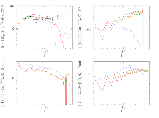
Figure 19: Initial guess (dashed line) and reconstructed (solid line) power spectra for each of reconstructed components obtained from the real data for case 1 at 50 GHz. The dotted lines correspond to the $1\sigma$ confidence level of the reconstructed power spectra. For comparison the power spectrum measurements obtained from the COBE-DMR data are also plotted in the CMB panel.

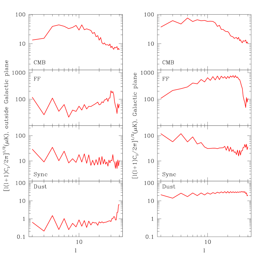
Figure 20: Reconstructed power spectra for case 1 inside and outside the galactic cut for real data.

6 Discussion and conclusions

We have presented a flexible MEM algorithm that combines the advantages of real (or data) space and harmonic space. On the one hand, the $\chi^{2}$ is calculated in data space, which allows one to include straightforwardly the properties of the noise as well as incomplete sky coverage. On the other hand, the entropy is estimated in harmonic space allowing easy introduction of available prior information about the power spectra of the components that we aim to reconstruct. In addition, the method takes into account correlations between different modes because we perform a single minimisation of $\sim n_{c}\ell_{max}^{2}$ variables instead of minimising mode-by-mode as in harmonic MEM. We perform this global minimisation using a Newton-Raphson method, which needs the Hessian matrix ${\mathbf{H}}$ to be evaluated and inverted. In practice, this is not feasible since we have a very large number of variables so we have approximated ${\mathbf{H}}$ by a block diagonal matrix, which gives very good results. Unfortunately, this minimisation is very time consuming and the method is many times slower than harmonic MEM.

To test the performance of the method we have applied it to simulated spherical data and then to real data. In particular, we have used the three frequency channels of COBE-DMR, the Haslam map and the lowest frequency map of COBE-DIRBE to reconstruct the CMB, free-free, synchrotron and dust emissions.

6.1 Analysis of simulated data

An important issue that has been thoroughly studied in the present work is the determination of the frequency dependence of the different components. We have modelled the free-free and synchrotron with a power law parametrised by indices $\beta_{\rm ff}$ and $\beta_{\rm syn}$ respectively and the dust by a grey body model with two parameters (the dust temperature $T_{d}$ and the dust emissivity $\alpha_{d}$). We have then applied the MEM algorithm to our simulated data (generated using $\beta_{\rm ff}=-0.16,\beta_{\rm syn}=-0.8,{\rm T}_{d}=18$ and $\alpha_{d}=2$) for many combinations of the spectral parameters and have studied the behaviour of different diagnostic quantities when the assumed values of these parameters depart from the true ones.

Firstly, we have studied a low noise case where the noise level of the COBE-DMR simulated maps have been lowered by a factor of 5. In this case we find that the $\chi^{2}$ value of the reconstructions can successfully identify the correct set of spectral parameters. In addition, we also find that there exists a high correlation between the error of the CMB reconstruction and other quantities that can be directly estimated from the reconstructed maps. In particular, together with the $\chi^{2}$ value, the entropy, the $\varphi$ function , the dispersion of the CMB reconstructed map, and the cross correlations between the reconstructed CMB and galactic components are good indicators of the quality of the reconstructions.

Secondly, we have applied MEM to our set of simulated data using realistic levels of noise for the same sets of spectral parameters. Due to the low signal to noise ratio of our data set, we find that the $\chi^{2}$ is not longer able to pick the right combination of spectral parameters. Therefore we have constructed an empirical selection function $G$ which is given by a linear combination of $\chi^{2}$, $|S|$, $\varphi$ , the dispersion of the CMB reconstructed map, and the cross correlations between the reconstructed CMB and galactic components. We pick as our best set of reconstructions the one with the lowest value of $G$. We have considerd a total of 81 different cases, with three possible values for each spectral parameter. Using the quantity $G$, we can clearly see that the correct dust model is clearly preferred over the others (see Fig. 8). However, it is very difficult to pick the correct values of the spectral indices for the free-free and synchrotron, since our data do not have enough information. In fact the quantity $G$ is almost identical for the 5 best cases due to the fact that our noisy data can accomodate a range of different spectral models. In any case, even if we can not determine unambiguosly the spectral parameters for the free-free and synchrotron component, the CMB reconstruction is very robust outside the galactic cut and the differences between the CMB reconstructions for the cases with lower values of $G$ are well within the statistical errors. In particular the level of the dispersion of the residuals of the smoothed 7 degree reconstructed CMB map outside the galactic cut ranges between 21.2 and 22.0 $\mu$K for all the cases between 1 and 30. To illustrate this point we can also look at the differences in the CMB reconstructed power spectra for the different cases. Fig. 21 shows the CMB power spectrum obtained for case 1 (solid line) versus the average power spectrum obtained from the 5 cases with lower values of $G$. The error bars correspond to the dispersion in the values of the $C_{\ell}$’s obtained from the former 5 cases. Note that this dispersion is very small, which shows that the recovered CMB power spectrum is also very robust for these 5 cases. This also indicates that, at least for ideal simulated foregrouns with spatially constant spectral parameters, the error introduced in the CMB power spectrum due to the wrong identification of these parameters (provided we pick one of the reconstructions with a lower value of $G$) is much smaller than the statistical error.

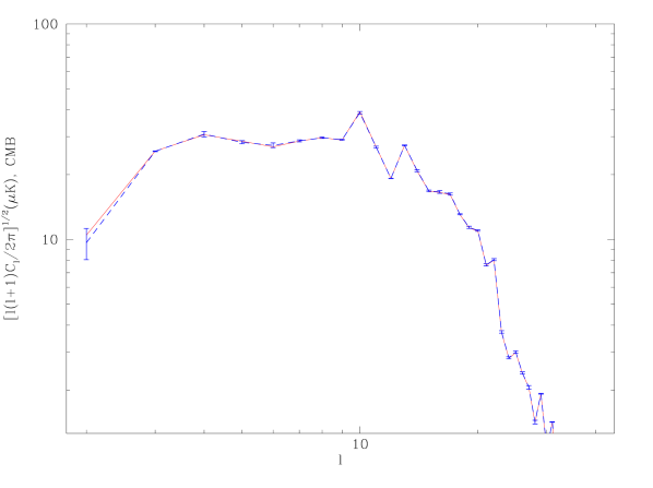
Figure 21: CMB reconstructed power spectrum for case 1 of the simulated data (solid line) and average CMB reconstructed power spectra for the 5 cases with a lower value of $G$ (dashed line). The error bars are the dispersion obtained from these 5 power spectra.

For case 1 (the case with the correct spectral parameters) we have found that the CMB error reconstruction for the (realistic) simulated data is at the level of 21 $\mu$K. The level of CMB residuals are comparable inside and outside the galactic cut, which indicates that the CMB has been equally well recovered in both regions of the sky. Note that the estimated error given by the method is $\sim 22\mu K$. The recovered CMB power spectrum follows the input one up to $\ell\sim 15$ and then starts to drop due to the resolution of the COBE-DMR data. This result is again comparable inside and outside the galactic plane. The free-free emission has been recovered with a residual error of $\sim 42\mu K$ in the galactic plane at 50 GHz. At high galactic latitude, the free-free reconstruction has basicly been lost. This result also shows in the reconstructed power spectrum, where we find a clear excess of structure at $\ell\ga 10$ outside the galactic cut, whereas MEM is able to recover it up to $\ell\sim 25$ inside the Galaxy. The synchrotron and dust emissions have been very well recovered in the galactic plane with errors of $\sim 3$ per cent and $\sim 0.2$ per cent, respectively. Outside the galactic cut the reconstruction is also quite good, at the level of $\sim 15$ per cent for the synchrotron and $\sim 5$ per cent for the dust. The whole-sky power spectra follows also quite faithfully the input one up to $\ell\la 30$ for the synchrotron and up to $\ell_{max}$ for the dust. However, the recovered dust power spectrum shows some excess at small scales when only the region outside the galactic cut is considered. Note that MEM has been able to recover the power spectra of the galactic components, independently of the supplied initial power spectra (dashed lines in Fig. 12), which was very far from the true one. We have tested that different initial power spectra lead to very similar reconstructions, provided MEM uses the iterative mode to obtain the correct power spectra.

6.2 Analysis of real data

In $\S$5 we have applied the same method to the true data. We have calculated the value of $G$ for a total of 180 different sets of spectral parameters in the range $-0.19\leqslant\beta_{\rm ff}\leqslant-0.13$, $-0.9\leqslant\beta_{\rm syn}\leqslant-0.6$, $16\leqslant T_{d}\leqslant 22$ and $1.6\leqslant\alpha_{d}\leqslant 2.2$. The best reconstructions are found for $\beta_{\rm ff}=-0.19$, $\beta_{\rm syn}=-0.8$, $T_{d}=19$ and $\alpha_{d}=2$. The cross correlations between the CMB and galactic components are at a similar level to those of the simulations (Fig. 15 versus Fig. 7). However, the value of $\varphi$, $\chi^{2}$, $|S|$, $\sigma_{CMB}^{rec}$ and thus of $G$ are a bit higher than the ones found for the simulated cases. This indicates that our model does not fit the data as well as in the ideal case. This is not surprising taking into account the large number of uncertainties of the data: the frequency dependence of the model, variation of the spectral parameters across the sky or in the frequency range or even the presence of some unknown component. In spite of this, we still have a reasonable fit to our data (the reduced $\chi^{2}$ is $\sim$ 1). As in the simulated case, some dust models are clearly favoured with respect to the others (Fig. 14) although the situation is not so clear as in the ideal case. Again this is due to all the uncertainties we have with respect to the frequency behaviour of the components which make the presence of degenerate cases even more important than in the simulated case.

The reconstructed maps for the four components are given in Fig. 17 for case 1 (the one with the lowest values of $G$) and the corresponding dispersions of the reconstructions as well as the estimated errors are shown in Table 8. From these results, we can see that there is some clear contamination of the CMB reconstruction in the galactic plane. For instance the dispersion of the recovered CMB is at the level of 35 $\mu$K outside the galactic cut, whereas in the galactic centre has a value of $\sim 47\mu$K. This is another indication of the fact that our model for the galactic components is not properly fitting the data. However, we believe that the reconstructed CMB sky outside the Galaxy is reasonably well recovered. Even if our assumptions about the spectral behaviour of the components are wrong, we have seen in the simulations that this had very little effect in the CMB reconstructed map outside the galactic cut, providing we are taking cases with low values of $G$. This is also happening when using real data. In particular, the difference between the 7 degree smoothed CMB restored maps at high galactic latitude for case 1 and all cases up to case 20 is $\la 3\mu$K. For the same cases, the differences are $\la 10\mu$K in the galactic plane, except for one of the cases. We have also plotted the average and the dispersion of the CMB recovered power spectrum for the 5 cases with a lower value of $G$ (Fig. 22). As in the simulated case, we find very little dispersion within these reconstructed power spectra, which confirms that the CMB reconstruction is not affected by certain variations on the spectral parameters.

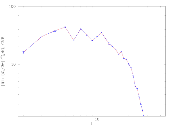
Figure 22: CMB reconstructed power spectrum for case 1 of the real data (solid line) and average CMB reconstructed power spectra for the 5 cases with lower values of $G$ (dashed line). The error bars are the dispersion obtained from these 5 power spectra.

As in the simulated case, the free-free emission has been recovered only in the galactic centre with a dispersion value at 50 GHz of $\sim 238\mu$K and with an estimated error of $\sim 48\mu$K. This value is several times higher than expected from $H\alpha$ measurements and raise again the issue of an unknown component. The synchrotron and dust reconstructions, however, look very good with estimated errors of $\sim 3$ and $\sim 1\mu$K respectively. These values account only for the statistical error but do not take into account the uncertainties coming from the determination of the spectral parameters.

As shown in Fig. 19 the CMB recovered power spectrum follows the shape of the measurements obtained from the COBE data, but with a slightly higher normalisation which indicates again the presence of some excess contamination in the recovered CMB map. This is confirmed by looking at the reconstructed CMB power spectrum inside and outside the galactic cut (Fig. 20). At the high galactic latitude region the amplitude of the $C_{\ell}$’s is consistent with the expected level whereas those obtained for the galactic plane present an excess of power. The free-free is recovered up to $\ell\la 30$ and then drops to zero, since the data do not have enough information at those scales. As in the simulated case, what seems a spurious excess of power is found at high $\ell$’s in the reconstructed power spectrum of the high galactic latitude region.

The recovered synchrotron power spectrum follows approximately the shape of the input power spectra (as expected since it has been obtained extrapolating the Haslam map) up to $\ell\la 25$ . For higher multipoles, the power spectra starts to oscillate which indicates that the reconstruction is not reliable at those scales. Finally, the dust emission seems to be well reconstructed up to the considered $\ell_{max}$ for the whole sky power spectrum. However, some excess is found at high $\ell$’s in the power spectrum obtained from the high galactic latitude region. We would like to point out that, as in the simulated case, changing the initial guess power spectra has very little effect in the reconstructions.

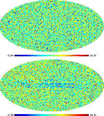
Figure 23: Normalised residual noise for the COBE-DMR 53 GHz channel for case 1 of simulated data (top) and of real data (bottom).

An extra check of the quality of the reconstructions can be performed by looking at the normalised residual noise for each frequency channel. This map is constructed by subtracting the predicted noiseless data (obtained using the reconstructed maps) from the actual noisy data. This gives the ‘predicted noise’ at the given frequency channel, which is then divided by the noise dispersion at each pixel. If the fit is acceptable this map should be a realisation of a Gaussian white noise field of unit dispersion with no visible structure, although one should be careful since incorrect choices of the spectral parameters can also give rise to this result due to degeneracies. As an illustration, the top panel of Fig. 23 shows the normalised residual noise for the 53 GHz frequency channel for case 1 of the simulations. No visible structure is present in the map, which confirms on the one hand, that the anisotropic noise has been properly taken into account and, on the other hand, that the Galaxy has been well fitted by our components. The bottom panel of the figure shows the same map for case 1 of the real data, which shows some visible structure in the galactic centre. This further confirms the fact that we are not fully subtracting the Galaxy.

6.3 Two-components dust model

This inability of the components to fit the data may be due either to variations of the spectral parameters with position or the frequency range, or to the fact that some other unknown component is needed to fit properly the data. A point raised by Jones et al. (1999) is the possiblity of reconstructing more than one dust component to account for spatially variations of the dust spectral parameters. Although each of the dust reconstructions may not have physical meaning, adding them together improved the reconstruction. Moreover, when a dust component with emissivity variations from pixel to pixel was included in the simulated data, the errors of the CMB reconstruction were also reduced by using three dust components with different emissivities, as compared with the case of reconstructing a single dust component whose emissivity was the average of the input template.

We have tested this possibility by adding to our set of data the second COBE-DIRBE channel (at 2141 GHz) and reconstructing two dust components. Since we have a total of 6 spectral parameters, it is not possible to cover exhaustively the full range of possible values. Instead, we have fixed the values of $\beta_{\rm ff}$, $\beta_{\rm syn}$ and $\alpha_{d}$ to the ones found to be optimal in $\S\ref{sec:freq_data}$ ($-0.19$, $-0.8$ and 2 respectively) and varied the dust temperatures of the two dust components in the range of 4 to 22 K. The best reconstruction was found for $T_{1}=20$ K and $T_{2}=11$ K with a value of $G=53.9005$. The CMB recovered map is given in the top panel of Fig. 25 and has been plotted in the same scale as the one of Fig. 17 to allow for a straightforward comparison. The middle panel shows the difference between the reconstructed CMB map using one dust component minus the one obtained with two dust components. It is obvious that the dispersion of the CMB map has been lowered inside the Galaxy (47.4 $\mu$K in the one dust component versus 42.4 $\mu$K in the two dust components) and the new CMB reconstruction seems to have less galactic contamination. This can also be seen in Fig. 24 which shows the power spectra of both reconstructions as well as the COBE-DMR data points.

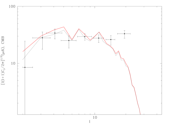
Figure 24: Power spectrum obtained from the (unsmoothed) CMB reconstruction of Fig. 17 (solid line) versus the power spectra of the recovered CMB obtained using two dust components (dotted line). The power spectrum measurements obtained from the COBE-DMR data are also plotted (solid squares).

The CMB reconstruction obtained using two dust components is closer to the measured power spectra. However, both maps are very similar outside the galactic cut. The dispersion of the difference map in this region is 5 $\mu$K, which is much lower than the estimated statistical error. The free-free and synchrotron reconstructed maps are very similar for both models, with differences $\sim$3 per cent for the free-free and $\sim$2 per cent for the synchrotron. The dust emission is now composed of the sum of two dust components. Each of them may not have a physical meaning but the extra degree of freedom should help to account for temperature variations of the dust component. In fact, the cold dust component presents negative as well as positive values in the reconstructed map and should be understood as a correction to the hot component, which helps to fit both of the COBE-DIRBE maps at high frequencies as well as some excess emission at lower frequencies. The total dust emission at 50 GHz is given in the bottom panel of Fig. 25. Note that the emission in the Galaxy centre has been extended with respect to the case when only a single dust component was used. Basically, the excess of emission of the CMB reconstructed map in the one single component case is being put into this cold dust component. Although this seems to improve the results, the normalised residual noise maps for the COBE-DMR frequency channels present some structure in the galactic centre and they look very similar to those obtained for the case of one single dust component (bottom panel of Fig. 23). Therefore, our model is still not fitting the Galaxy properly and a more exhaustive analysis should be performed in order to determine the correct spectral dependences of the components of the microwave sky.

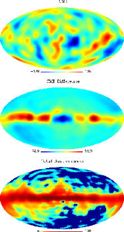
Figure 25: Top panel: CMB reconstructed map at 50 GHz smoothed with a 7 degree Gaussian beam for the case when 2 dust components have been used. Middle panel: map resulting of subtracting the previous reconstruction from the one of Fig. 17. Bottom panel: total dust emission at 50 GHz obtained by adding the contribution from the two dust components smoothed with a 7 degree Gaussian beam (non-linear scale). The CMB and dust reconstructions have been plotted in the same scale as the corresponding reconstructions of Fig. 17. Units are $\mu$K (thermodynamical temperature).

Another possible explanation for the difficulty in fitting the data with our model is the presence of an unknown component. As already mentioned, several works have found an anomalous galactic emission at low frequency, which correlates with the thermal dust one. Although in principle a free-free component is fitting the data that we have used, its amplitude is higher than expected from estimations based on the H_α emission. The spectral index found for the free-free was also slightly higher than expected from theoretical predictions. As a test, we have also run the code for a few models with $\beta_{\rm ff}=-0.22$, two of which gave slightly lower values of $G$ than the chosen model. However, the synchrotron map was presenting negative features in the Galaxy, which is indicative of a degeneracy between the spectral parameters.

To account for this anomalous component, we have tried to fit for a spinning dust component using the extra COBE-DIRBE channel in addition to the CMB, free-free, synchrotron and (thermal) dust emissions. The spectral parameters have been fixed to the values found in $\S\ref{sec:freq_data}$. We have tried three different spinning dust models which correspond to the cold neutral medium, the warm neutral medium (described in Draine & Lazarian, 1998) and a combination of both. In the three considered cases, the $G$ value was appreciably higher than in the optimal case and the CMB reconstruction was lost. However, even if spinning dust were present in the data, it would have been very difficult to recover it. We are basically trying to reconstruct three components, CMB, free-free and spinning dust from just the 3 COBE-DMR channels, which are very noisy, and therefore the data just do not have enough information. Moreover, a wider range of frequencies (between 5 and 60 GHz) would be necessary to distinguish between spinning dust and the other galactic components.

Finally, we would like to point out that the combination of MEM and other reconstruction methods should also be investigated in the future. In particular, blind source separation methods can infer the spectral dependence of the reconstructed components under certain assumptions. This information could be used as input for the MEM algorithm, which would improve the results of each method alone.

Appendix A $\chi^{2}$ function and derivatives

In order to evaluate the $\chi^{2}$ in real space we need to be able to predict the data at each pixel from the hidden variables ${\mathbf{h}}_{\ell m}$. The temperature field at a given pixel is normally written in terms of spherical harmonic coefficients. So, at a position $i$ corresponding to angles $(\theta,\phi)$ and at frequency $\nu$, the predicted noiseless data $d^{p}_{\nu}$ can be written as

$$d^{p}_{\nu}(\theta,\phi)=\sum_{\ell=0}^{\ell_{max}}\sum_{m=-\ell}^{\ell}a_{\ell m}^{\nu}Y_{\ell m}(\theta,\phi),$$ (17)

where $a_{\ell m}^{\nu}$ are the predicted harmonic coefficients at frequency $\nu$ and the $Y_{\ell m}$ are the spherical harmonics:

$$Y_{\ell m}(\theta,\phi)=\left[\frac{2\ell+1}{4\pi}\frac{(\ell-m)!}{(l+m)!}\right]^{1/2}P_{\ell m}(\cos\theta)e^{im\phi}.$$ (18)

Taking into account that, for a real field, we have $a_{\ell-m}=(-1)^{m}a_{\ell m}^{*}$, we can write $d_{\nu}$ as

$$d^{p}_{\nu}(\theta,\phi) = \sum_{\ell=0}^{\ell_{max}}\sum_{m=0}^{\ell}k_{m}\left[\Re(a_{\ell m}^{\nu})\cos(m\phi)\right.$$ (19)

$$-\Im(a_{\ell m}^{\nu})\sin(m\phi)\left.\right]\Lambda_{\ell m}$$

where $k_{m}=1$ for $m=0$ and $k_{m}=2$ otherwise. $\Lambda_{\ell m}$ denotes the factor that multiplies the exponential in the $Y_{\ell m}$ expression. The $a_{\ell m}^{\nu}$ are related to the hidden variables $\mathbf{h_{\ell m}}$ by:

$$a_{\ell m}^{\nu}=\sum_{\nu}B_{\ell}^{\nu}({\mathbf{F}}{\mathbf{L}}_{\ell}{\mathbf{h}}_{\ell m})_{\nu},$$ (20)

where we have assumed that the beam is spherically symmetric. $B_{\ell}^{\nu}$ is the beam in harmonic space at frequency $\nu$, ${\mathbf{F}}$ is the conversion $n_{f}\times n_{c}$ matrix. which encodes the frequency dependence of the components, ${\mathbf{L}}_{\ell}$ is the Cholesky decomposition (an $n_{c}\times n_{c}$ matrix) and ${\mathbf{h}}_{\ell m}$ is the column vector containing the hidden modes for each of the microwave components. The $\chi^{2}$ function is then written as

$$\chi^{2}=\sum_{\nu=1}^{n_{f}}\sum_{i=1}^{N_{p}}\frac{\left[d_{\nu,i}^{o}-d^{p}_{\nu,i}({\mathbf{h}}_{\ell m})\right]^{2}}{\sigma_{\nu,i}^{2}},$$ (21)

where $N_{p}$ is the number of pixels of each data map, $d_{\nu,i}^{o}$ is the observed data at frequency $\nu$ and pixel $i$ and $\sigma_{\nu,i}$ is the noise dispersion at frequency $\nu$ and pixel $i$.

If we denote $r_{\ell m}^{c}$ and $j_{\ell m}^{c}$ as the real and imaginary parts of the hidden harmonic coefficients for component $c$, we can write the first derivatives of $\chi^{2}$ as

$$\frac{\partial\chi^{2}}{\partial r_{\ell m}^{c}} = -2k_{m}\sum_{\nu=1}^{n_{f}}\sum_{i=1}^{N_{p}}\frac{d_{\nu,i}^{o}-d^{p}_{\nu,i}}{\sigma_{\nu,i}^{2}}$$

$$\times\cos(m\phi_{i})\Lambda_{\ell m}B_{\ell}^{\nu}(FL)_{\nu c},$$

$$\frac{\partial\chi^{2}}{\partial j_{\ell m}^{c}} = 2k_{m}\sum_{\nu=1}^{n_{f}}\sum_{i=1}^{N_{p}}\frac{d_{\nu,i}^{o}-d^{p}_{\nu,i}}{\sigma_{\nu,i}^{2}}$$ (22)

$$\times\sin(m\phi_{i})\Lambda_{\ell m}B_{\ell}^{\nu}(FL)_{\nu c}.$$

The second derivatives are given by

$$\frac{\partial^{2}\chi^{2}}{\partial r_{\ell m}^{c}\partial r_{\ell m}^{c^{\prime}}} = 2k_{m}^{2}\sum_{\nu=1}^{n_{f}}\sum_{i=1}^{N_{p}}\frac{1}{\sigma_{\nu,i}^{2}}\left[\cos(m\phi_{i})\Lambda_{\ell m}B_{\ell}^{\nu}\right]^{2}$$

$$\times(FL)_{\nu c}(FL)_{\nu c^{\prime}},$$

$$\frac{\partial^{2}\chi^{2}}{\partial j_{\ell m}^{c}\partial j_{\ell m}^{c^{\prime}}} = 2k_{m}^{2}\sum_{\nu=1}^{n_{f}}\sum_{i=1}^{N_{p}}\frac{1}{\sigma_{\nu,i}^{2}}\left[\sin(m\phi_{i})\Lambda_{\ell m}B_{\ell}^{\nu}\right]^{2}$$ (23)

$$\times(FL)_{\nu c}(FL)_{\nu c^{\prime}}.$$

These second derivatives of $\chi^{2}$ are the main contribution to the second derivatives of $\varphi=\chi^{2}-\alpha S$, since the term coming from the entropy is generally much smaller. They are also the main contribution to the Hessian, since we are assuming that we can neglect the rest of the elements. Note that these derivatives are all positive and therefore $\varphi$ will have a well defined minimum in the $\mathbf{h_{\ell m}}$ space. This means that the Newton-Raphson (NR) method will always be driven in the right direction and should be able to find the desired global minimum. Note also that the second derivatives of $\chi^{2}$ depend only on the characteristics of the experiment, on the assumed spectral parameters and also in the initial power spectra but they are independent of the $h_{\ell m}$. Therefore we do not need to reevaluate these derivatives at each NR iteration.

References

- [1] Baccigalupi C., Bedini L., Burigana C., De Zotti G., Farusi A., Maino D., Maris M., Perrota F., Salerno E., Toffolatti L., Tonazzini A., 2000, MNRAS, 318, 769
- [2] Banday A.J., Gorski K.M., Bennett C.L., Hinshaw G., Kogut A., Lineweaver C., Smoot G.F., Tenorio L., 1997, ApJ, 475, 393
- [3] Banday A.J. & Wolfendale A.W., 1991, MNRAS, 245, 462
- [4] Barreiro R.B., Sanz J.L., Herranz D. & Martínez-González E., 2003, MNRAS, 342, 119
- [5] Bennett C.L. et al., 1996, ApJ, 464, L1
- [6] Bennett C.L. et al., 2003a, ApJS, 148, 1
- [7] Bennett C.L. et al., 2003b, ApJS, 148, 97
- [8] Benoit A. et al., 2003, A&A, 399, L19
- [9] Bouchet F.R., Gispert R. & Puget J.L., 1996, in Dwek E., ed,. Proc. AIP Conf. 348. The mm/sub-mm foregrounds and future CMB space missions. AIP Press, New York, p.255
- [10] Cayón L., Sanz J.L., Barreiro R.B., Martínez-González E., Vielva P., Toffolatti L., Silk J., Diego J.M. & Argüeso F., 2000, MNRAS, 315, 757
- [11] Delabrouille J., Cardoso J.F. & Patanchon G., 2003, MNRAS, 346, 1089
- [12] Dennison B., Simonetti J.H. & Topasna G., 1998, Publ. Astron. Soc. Australia, 15, 147
- [13] de Oliveira-Costa A., Kogut A., Devlin M.J., Netterfield C.B., Page L.A & Wollack E.J., 1997, ApJ, 482, 17
- [14] de Oliveira-Costa A., Tegmark M., Gutiérrez C.M., Jones A.W., Davies R.D., Lasenby A.N., Rebolo R. & Watson R.A., 1999, ApJ, 527, L9
- [15] Desert F.-X., Boulanger F. & Puget J.L., 1990, A&A, 237, 215
- [16] Dickinson C., Davies R.D. & Davis R.J., 2003, MNRAS, 341, 369
- [17] Diego J.M., Vielva P., Martínez-González E., Silk J., Sanz J.L., 2002, MNRAS, 336, 1351
- [18] Draine B.T. & Lazarian A., 1998, ApJ, 494, L19
- [19] Finkbeiner D.P., 2003, ApJS, 146, 407
- [20] Finkbeiner D.P., Davis M. & Schlegel D.J., 1999, ApJ, 524, 867
- [21] Finkbeiner D.P., Schlegel D.J, Frank C. & Heiles C., 2002, ApJ, 566, 898
- [22] Gaustad J.E., McCullough P.R., Rosing W. & Van Buren D., 2001, PASP, 113, 1326
- [23] Giardino G., Banday A.J., Górski K.M., Bennett K., Jonas J.L. & J. Tauber, 2002, A&A, 387, 82
- [24] Górski K.M., Wandelt B.D., Hansen F.K., Hivon E. & Banday A.J., 1999, in astro-ph/9905275
- [25] Grainge K. et al., 2003, MNRAS, 341, L23
- [26] Halverson W., et al., 2002, ApJ, 568, 38
- [27] Hanany S., et al. 2000, ApJ, 545, L5
- [28] Haslam C.G.T., Salter C.J., Stoffel H. & Wilson W.E., 1982, A&AS, 47, 1
- [29] Herranz D., Gallegos J., Sanz J.L. & Martínez-González E., 2002a, MNRAS, 334, 533
- [30] Herranz D., Sanz J.L., Barreiro R.B. & Martínez-González E., 2002b, ApJ, 580, 610
- [31] Herranz D., Sanz J.L., Hobson M.P., Barreiro R.B., Diego J.M., Martínez-González E. & Lasenby A.N., 2002c, MNRAS, 336, 1057
- [32] Hobson M.P., Jones A.W., Lasenby A.N. & Bouchet F.R., 1998, MNRAS, 300, 1 (H98)
- [33] Hobson M.P., Barreiro R.B., Toffolatti L., Lasenby A.N., Sanz J.L., Jones A.W. & Bouchet F.R., 1999, MNRAS. 306, 232
- [34] Hobson M.P., McLachlan C., 2003, MNRAS, 338, 765
- [35] Jonas J.L., Baart E.E. & Nicholson G.D., 1998, MNRAS, 297, 997
- [36] Jones A.W., Hobson M.P., Mukherjee P. & Lasenby A.N., 2000, ApL&C, 37, 369
- [37] Kogut A., 1999, ASP Conf. Series, 181, 91
- [38] Kogut A., Banday A.J., Bennett C.L., Górski K.M., Hinsaw G. & Reach W.T., 1996, ApJ, 460, 1
- [39] Kuo C.L. et al., 2004, ApJ, 600, 32
- [40] Leitch E.M., Readhead A.C.S., Pearson T.J. & Myers S.T., 1997, ApJ, 486, 23
- [41] Maino D., Farusi A., Baccigalupi C., Perrotta F., Banday A.J., Bendini L., Burigana C., De Zotti G., Górski K.M. & Salerno, E., 2002, MNRAS, 334, 1, 53
- [42] Martínez-González E., Diego J.M., Vielva P. & Silk J., 2003, MNRAS, 345, 1101
- [43] Mason B.S. et al., 2003, ApJ, 591, 540
- [44] Netterfield C.B., et al., 2002, ApJ, 571, 604
- [45] Reich P. & Reich W., 1986, A&A, 63, 205
- [46] Reich P. & Reich W., 1988, A&A, 74, 7
- [47] Reynolds R.J., Haffner L.M. & Madsen G.J., 2002, in ASP Conf. Ser. 282, Galaxies: The Third Dimension, ed. M. Rosado, L. Binette, & L. Arias (San Francisco: ASP), 31
- [48] Sanz J.L., Herranz D., Martínez-González E., 2001, ApJ, 552, 484
- [49] Schlegel D.J., Finkbeiner D.P. & Davis M., 1998, ApJ, 500, 525
- [50] Smoot G., 1998, in astro-ph/9801121
- [51] Stolyarov V., Hobson M.P., Ashdown M.A.J. & Lasenby A.N., 2002, MNRAS, 336, 97 (S02)
- [52] Stolyarov V., Vielva P., Barreiro R.B., Hobson M.P., Martínez–González E.& Lasenby A.N., 2003, in preparation
- [53] Tegmark M. & de Oliveira-Costa A., 1998, ApJ, 500, 83
- [54] Tegmark M. & Efstathiou G., 1996, MNRAS, 281, 1297
- [55] Tegmark M. & Hamilton A., 1997, in proccedings of the 18th Texas Symposium on Relativistics Astrophysics & Cosmology, eds A. V. Olinto, J. A. Frieman & D. N. Schramm, p270 (World Scientific)
- [56] Vielva P., Martínez-González E., Cayón L., Sanz J.L. & Toffolatti L., 2001a, MNRAS, 326, 181
- [57] Vielva P., Barreiro R.B., Hobson M.P., Martínez–González E., Lasenby A.N., Sanz J.L. & Toffolatti L., 2001b, MNRAS, 328, 1
- [58] Vielva P., Martínez-González E., Gallegos J.E., Toffolatti L. & Sanz J.L., 2003, MNRAS, 344, 89
- [59] Wright E.L., Smoot G.F., Kogut A., Hinshaw G., Tenorio L., Lineweaver C., Bennett C. L. & Lubin, P. M., 1994, ApJ, 420, 1