Dark Energy, Expansion History of the Universe, and SNAP

Abstract

This talk presents a pedagogical discussion of how precision distance-redshift observations can map out the recent expansion history of the universe, including the present acceleration and the transition to matter dominated deceleration. The proposed Supernova/Acceleration Probe (SNAP) will carry out observations determining the components and equations of state of the energy density, providing insights into the cosmological model, the nature of the accelerating dark energy, and potentially clues to fundamental high energy physics theories and gravitation. This includes the ability to distinguish between various dynamical scalar field models for the dark energy, as well as higher dimension and alternate gravity theories. A new, advantageous parametrization for the study of dark energy to high redshift is also presented.

I Introduction

Little else evokes the recent great advances in our abilities in cosmological observations like the quest to explore the expansion history of the universe. This carries cosmology well beyond “determining two numbers” – the present dimensionless density of matter $\Omega_{m}$ and the present deceleration parameter $q_{0}$ of Sandage san61 – to seeking to reconstruct the entire function $a(t)$ representing the expansion history of the universe. In the previous case cosmologists sought only a local measure – the first two derivatives of the scale factor $a$, evaluated at a single time $t_{0}$ – while in the latter case we strive to map out the function determining the global dynamics of the universe.

While many qualitative elements of cosmology follow merely from the form of the metric, i.e. the kinematical cosmology (see Weinberg wein ), deeper understanding of our universe requires knowledge of the dynamics, the quantitative role of gravitational forces determining the scale factor evolution, $a(t)$. This echoes the flows of energy between components, e.g. the epoch of radiation domination transitioning to that of matter domination, and is a key element in the growth of density perturbations into structure. Yet until recently the literature tended to consider only

$$H_{0}=(\dot{a}/a)_{0}\qquad;\qquad q_{0}=-(a\ddot{a}/\dot{a}^{2})_{0}\,,$$ (1)

the Hubble constant and the deceleration parameter today.

Now a myriad of cosmological observational tests can probe the function $a(t)$ more fully, over much of the age of the universe (see Sandage san88 , Linder lin89 ; lin97 , Tegmark teg ). All that is required is a probe capable, not just in theory but in practice, of observations both precise and accurate enough. A number of promising methods are being developed, but this talk concentrates on the most advanced, the magnitude-redshift relation of Type Ia supernovae.

The goal of mapping out the recent expansion history of the universe has several motivations. The thermal history of the universe, extending back through structure formation, matter-radiation decoupling, radiation thermalization, primordial nucleosynthesis, etc. has taught us an enormous amount about both cosmology and particle physics. It has spin offs in high energy physics, neutrino physics, gravitational physics, nuclear physics, and so on (see, e.g., Kolb and Turner kt ). The recent expansion history of the universe promises similarly fertile ground with the discovery of the current acceleration of the expansion of the universe. This involves concepts of the late time role of high energy field theories in the form of possible quintessence, scalar-tensor gravitation, higher dimension theories, brane worlds, etc.

Looking literally to the future, this accelerated expansion moreover has profound implications for the fate of the universe, from the viability of string theory string to eternal inflation and the heat death of the universe krauss to ideas on the cyclic nature of time stein . The recent expansion history offers guidance on the fate of our universe plus physics at the extremes: the form of high energy physics, physics at the smallest scales and in extra dimensions, physics in the most distant past and asymptotic future.

Section II considers the use of supernova observations to obtain the magnitude-redshift law out to $z\approx 2$ and how to relate this to the scale factor-time behavior $a(t)$. Section III presents specifics on the proposed Supernova/Acceleration Probe mission snap and its capabilities. Different parametrizations of the dynamics are investigated in Section IV, including extensions to nonstandard gravitation that alters the Friedmann equation governing the expansion evolution. Section V considers constraints from other probes, especially on the age of the universe and the Hubble constant.

The reconstruction of the recent expansion history, à la Figure 5, may hopefully soon be a standard feature of future textbooks.

II Mapping the Expansion History

First we consider the global description: the geometry of the universe and the form of the spacetime metric that this imposes. Readers familiar with cosmology might wish to skip this didacticism and proceed to either Eq. 2 or 6.

Precision measurements of the cosmic microwave background (CMB) radiation temperature across the entire sky, as well as subsidiary experiments such as radio source counts, galaxy counts, and background radiation surveys in other wavelength bands, indicate our universe is very well modeled by an isotropic spacetime. Redshift surveys such as the 2dF and Sloan Digital Sky Survey allow us to begin to construct a three dimensional picture of the universe to test homogeneity directly. CMB fluctuation measurements can constrain inhomogeneous models as well. Moreover, we can always fall back upon the Cosmological Principle, which provides a strong theoretical expectation that the isotropy observed about us can be interpreted as about a random location and therefore enforces global homogeneity. Ellis et al. ell have quantified the extent to which this could break down and shown that formally isotropy about any three points leads to homogeneity.

A homogeneous and isotropic universe is described within general relativity by the Robertson-Walker metric. This contains only two parameters – a function $a(t)$ and a constant $k$ – describing respectively the scale evolution or dynamics, and the spatial curvature. CMB measurements have further put tight constraints on the spatial curvature, restricting its characteristic scale today to be of order ten times the horizon scale, i.e. its effective energy density is at most of order 1% of the total energy density.

Thus for the rest of this paper we adopt the Robertson-Walker metric with flat spatial sections, $k=0$:

$$ds^{2}=-dt^{2}+a^{2}(t)[dr^{2}+r^{2}(d\theta^{2}+\sin^{2}\theta\,d\phi^{2})]\,.$$ (2)

We will also find it convenient sometimes to use conformal time $d\eta=dt/a$.

Type Ia supernovae, or any standardizable candles (sources with known luminosity), are excellently suited to map the expansion history $a(t)$ since there exists a direct relation between the observed distance-redshift relation $d(z)$ and the theoretical $a(t)$. The scale factor $a$ trivially translates into the observable redshift $z$ of the source by $a=(1+z)^{-1}$. That is, the expansion of spacetime directly stretches the wavelengths of the emitted light. On the other hand, that light was emitted a finite time ago since it had to traverse a certain distance $d$ from the supernova to the observer. The received energy flux from the supernova obeys the (relativistic) inverse square law, so the distance can be derived from the observed flux by relating it to the known emitted flux. Via the speed of light the distance is translated into a “lookback time” $t$. Thus one can proceed very simply from observables $d(z)$ to the expansion $a(t)$.

Mathematically, things are almost as simple. The relation between the scale factor and redshift holds for any “quiet” universe where the light from a source moving at velocities slow compared to the Hubble velocity (which is near unity for the distant sources used) propagates without interaction in an adiabatically evolving background. The distance used is the luminosity distance $d_{L}$, which is related to the coordinate distance appearing in the metric (2) by $d_{L}=(1+z)r$. All that remains is to find $r(z)$.

The form of $r(z)$ comes from light following null geodesics, $ds=0$. Thus $dr=dt/a=d\eta$ and

$$r(z)=\eta(z)=\int_{a_{e}}^{1}da/(a^{2}H)=\int_{0}^{z}dz^{\prime}/H(z^{\prime})\,,$$ (3)

where the Hubble parameter (a function now, not a single number) is $H=\dot{a}/a$ and $a_{e}=1/(1+z)$ is the scale factor at the time of emission, i.e. when the supernova exploded. This is the kinematical result, following purely from the geometry. To evaluate the function we need to introduce dynamics: equations of motion derived from the gravitation theory.

In general relativity these are known as the Friedmann equations and the relevant one relating the Hubble parameter to the matter and energy contents of the flat universe is

$$H^{2}=(8\pi/3)\rho\,.$$ (4)

The conservation condition of each (noninteracting) component is

$$\dot{\rho}/\rho=-3H(1+p/\rho)\equiv-3H[1+w(z)],$$ (5)

where the energy density is $\rho$, the pressure $p$, and the equation of state (EOS) of each component is defined by $w=p/\rho$. Ordinary nonrelativistic matter has $w=0$; a cosmological constant has $w=-1$. We explicitly allow the possibility that $w$ evolves. The total density and pressure are just the sum of the individual components.

Once one has $H(z)$ one can map out the expansion history $a(t)$ by

$$t(a)=\int_{a}^{1}da^{\prime}/(a^{\prime}H)=\int_{0}^{z}dz^{\prime}/[(1+z^{\prime})H(z^{\prime})].$$ (6)

The gross behavior of the scale factor over the entire age of the universe is illustrated in Figure 1. Note that the lookback time is zero at $z=0$ ($a=1$). One can classify expanding cosmologies into open, closed, and critical cases, and those which possessed a Big Bang vs. bounce models. To set the stage by adding one level of detail at a time, we are next interested in discrimination between models which have less extreme asymptotic behaviors. A blowup of the past history of simple models appears in Figure 2. The main focus of this paper though is a much finer discrimination, between models distinguished by small differences in their components. This is probed through the recent expansion history.

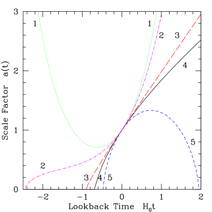
Figure 1: Overall expansion histories of expanding universes are sorted into classes: 1) a bounce model, 2) a loitering Eddington-Lemaître model, 3) an open model, 4) a critical, Einstein-de Sitter model, 5) a closed model.

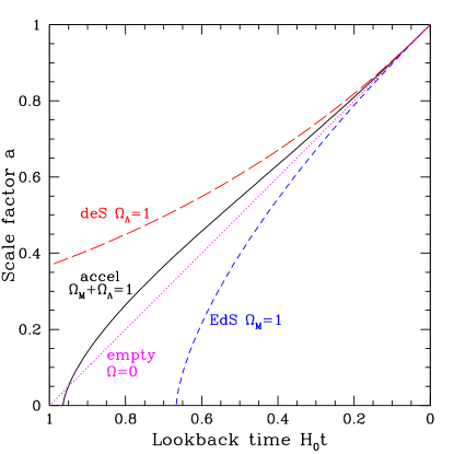
Figure 2: A more refined picture of the expansion history shows the differences between matter dominated (flat, Einstein-de Sitter), empty ($\Omega=0$, Milne), cosmological constant dominated (de Sitter), and presumably our universe (solid line): an accelerating model with both matter and dark energy.

III SNAP Capabilities

The distance-redshift relation can map out the expansion history. From the ability of supernovae, or other probes, to observe $r(z)$ one can fit and constrain $\rho$ and $w(z)$ of each component. To investigate the dark energy and distinguish between classes of physics models we need to probe the expansion back into the deceleration epoch, indeed over a redshift baseline reaching $z>1.5$ (see Fig. 3; Li01 ; HL02 ). SNAP snap is a simple, dedicated experiment specifically designed to map the distance-redshift relation out to $z=1.7$ with high precision and tight control of systematic errors.

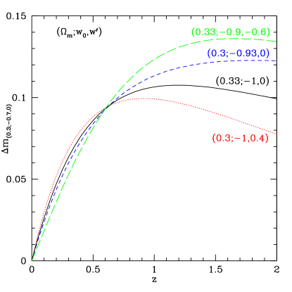
Figure 3: Degeneracies due to the dark energy model and the cosmological model cannot be resolved at low redshifts. In this differential magnitude-redshift diagram the three parameters to be determined are varied two at a time. Only at $z\approx 1.7$ do these very different physics models first exceed 0.02 mag discrimination. From HL02 .

These data can determine the cosmological parameters with high precision: depending on the exact model, the mass density $\Omega_{m}$ to $\pm 0.01$, vacuum energy density $\Omega_{\Lambda}$ and curvature $\Omega_{k}$ to $\pm 0.03$, and the dark energy equation of state $w$ to $\pm 0.05$ and its time variation $w^{\prime}=dw/dz$ to $\pm 0.3$. This time variation is a crucial distinguishing feature, not only for ruling out a cosmological constant explanation, but for guidance on the proper class of high energy physics theory to pursue. In addition, wide area weak gravitational lensing studies with SNAP will map the distribution of dark matter in the universe and teach us about the evolution of the nonlinear mass power spectrum.

The SNAP mission concept is a 2.0 meter space telescope with a nearly one square degree field of view. A half billion pixel, wide field imaging system comprises 36 large format new technology CCD’s and 36 HgCdTe infrared detectors. Both the imager and a low resolution ($R\sim 100$) spectrograph cover the wavelength range 3500 - 17000 Å, allowing detailed characterization of Type Ia supernovae out to $z=1.7$.

As a space experiment SNAP will be able to study supernovae over a much larger range of redshifts than has been possible with the current ground-based measurements – over a wide wavelength range unhindered by the Earth’s atmosphere and with much higher precision and accuracy. Many of these systematics-bounding measurements are only achievable in a space environment with low sky noise and a very small and stable point spread function (critical for lensing as well). Unlike other cosmological probes, supernova studies have progressed to the point that a detailed catalog of known and possible systematic uncertainties has been compiled – and, more importantly, approaches have been developed to constrain each one.

An array of data (e.g. supernova risetime, early detection to eliminate Malmquist bias, lightcurve peak-to-tail ratio, identification of the Type Ia-defining Si II spectral feature, separation of supernova light from host galaxy light, and identification of host galaxy morphology, etc.) makes it possible to study each individual supernova and measure enough of its physical properties to recognize deviations from standard brightness subtypes. For example, an approach to the problem of possible supernova evolution uses the rich stream of information that an expanding supernova atmosphere sends us in the form of its spectrum. A series of measurements will be constructed for each supernova that define systematics-bounding subsets of the Type Ia category. Only the change in brightness as a function of the parameters classifying a subtype is needed, not any intrinsic brightness. By matching like to like among the supernova subtypes, we can construct independent Hubble diagrams for each, which when compared bound systematic uncertainties at the targeted level of 0.02 magnitudes.

With a prearranged photometric observing program one obtains a uniform, standardized, calibrated dataset for each supernova, allowing for the first time comprehensive comparisons across complete sets of supernovae. The observing requirements also yield data ideal as survey images, and one automatically obtains host galaxy luminosity, colors, morphology, and type – a rich resource 9000 times larger than the Hubble Deep Field and somewhat deeper. Thus SNAP will map the distance-redshift relation and much more.

IV Modeling the Dynamics

A fly in the theoretical ointment is that the measured distance $r(z)$ is related to, but is not, the desired history relation $a(t)$. So we need to translate $r(z)$ into $a(t)$; this requires an intermediate step of obtaining $H(z)$. We can do this either directly or through the cosmology parameters $\rho$ and $w(z)$. The direct method involves a derivative of $r(z)$, so noisy data can introduce difficulties astier ; ht . We examine this approach further in §IV.3. First we discuss the reconstruction of $H(z)$ from the fit of the cosmological parameters to the observations.

Observational evidence for accelerated expansion informs us that (within the dark energy picture; cf. §IV.5) there must be further cosmological parameters, describing another component with a strongly negative EOS.

Assuming that just these two components, matter and another with EOS $w(z)$, control the dynamics during the epoch of interest, we obtain a solution for $H(z)$ and hence $r(z)$ by combining equations (3)-(5):

$$H_{0}r(z) = \int_{0}^{z}dz^{\prime}\,\Big{[}\Omega_{m}(1+z^{\prime})^{3}+(1-\Omega_{m})$$ (7)

$$\times e^{3\int_{0}^{\ln(1+z^{\prime})}d\ln(1+z^{\prime\prime})[1+w(z^{\prime\prime})]}\Big{]}^{-1/2},$$

where $\Omega_{m}$ is the dimensionless matter density $8\pi\rho_{m}/(3H_{0}^{2})$ and $H_{0}$ is the Hubble constant – the present value of the Hubble parameter. Equation (6) can then be used to obtain $a(t)$.

The EOS $w(z)$ is derived from the Lagrangian for that component, i.e. the particle physics enters here. One could solve the scalar field equation for a particular model to find $w(z)$ but then one does not obtain a model independent parameter space in which to compare models. For generality of treatment, various parametrizations of $w(z)$ are used (though hutstar introduces a principal component approach). We discuss a standard form next and a new parametrization in §IV.2.

IV.1 Linear $w(z)$

The conventional first order expansion to the EOS, enlarging the phase space to incorporate the critical property of time variation in the EOS, is $w(z)=w_{0}+w_{1}z$. In this case the exponential in (7) resolves to $(1+z)^{3(1+w_{0}-w_{1})}e^{3w_{1}z}$. Figure 4 illustrates the effect of changing the cosmological parameters, one at a time, on the expansion history.

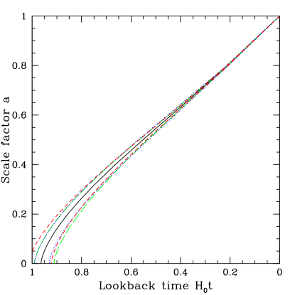
Figure 4: Precision experiments are necessary to differentiate the expansion histories of models with different densities and equations of state. The central curve is the history of a flat $\Omega_{m}=0.3$ model with cosmological constant. The red dashed curves vary the matter density by $\pm 0.05$, the blue dotted ones vary the equation of state of dark energy by $\pm 0.2$, and the green long dashed curves put in a time variation of the dark energy EOS, $dw/dz=\pm 0.5$.

An important point is the presence of correlation between the parameters $\Omega_{m}$, $w_{0}$, $w_{1}$ (see, e.g., welal ) which must be treated properly if more than one is allowed to vary (which is of course the general case). Figure 5 shows the reconstructed expansion history for a simulation of the future SNAP experiment. Despite it being able to determine each parameter individually to high precision, e.g. $\Omega_{m}$ to 0.03, $w_{0}$ to 0.05, $w_{1}$ to 0.3 (each marginalized over others), the correlations among them (i.e. degeneracies among their combinations) relax the tightness of the constraint SNAP would place on the expansion history. This is unavoidable (but see §IV.4).

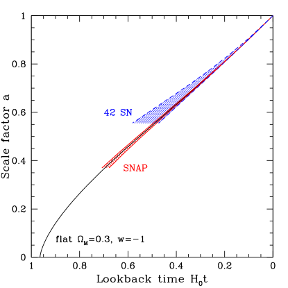
Figure 5: The constraints that supernova mapping of the expansion history through the magnitude-redshift relation provide. SNAP limits represent a generational advance in understanding the recent history of the universe.

IV.2 A new parametrization of the dark energy

Mapping the expansion history out to redshifts $z>1$, beyond the deceleration-acceleration transition represents a major advance in our cosmological knowledge. But high redshift does introduce complications in the parametrization of dark energy. In order to draw model independent constraints, we had parametrized the dark energy EOS linearly in redshift: $w(z)=w_{0}+w_{1}z$. This clearly grows increasingly problematic at redshifts $z>1$. However exact solutions for the EOS from the scalar field equations of motion do not allow us to make model independent statements.

Corasaniti and Copeland cc originally suggested an alternate parametrization in terms of a 7-dimensional phase space: the value of the EOS today, $w_{0}$, the values deep in the matter (radiation) dominated tracker regime, $w_{m}$ ($w_{r}$), the scale factors $a_{cm}$ ($a_{cr}$) at the time the field leaves the tracking behaviors, and the widths $\Delta_{m}$ ($\Delta_{r}$) of those transitions in Hubble units. They find success in a particular functional approximation with scale factor, obtaining the EOS $w(z)$ to better than 5% back to the last scattering surface for a range of models that display tracker behavior (where the field is in a slow roll regime that keeps the EOS nearly constant, determined by the EOS of the background component). Indeed they extend this function back into the radiation dominated epoch as well. While this only applies to dark energy field theories that have a slow roll regime, within that fairly varied class (e.g. potentials with inverse power laws, double exponentials, supergravity inspired models, etc.) it provides a model independent method of characterizing the behavior.

Such generality, while impressive, is somewhat unwieldy. For our present purposes we can make two simplifications. First, since we aim only to trace the expansion history back to the matter dominated epoch (for now at least), I simplify the phase space to four dimensions and obtain a fitting function for $w(a)$ as

$$w(a) = F+G\,\left[1+e^{-(a-a_{c})/\Delta}\right]^{-1}$$ (8)

$$F = w_{0}-(w_{m}-w_{0})(1+e^{-a_{c}/\Delta})(e^{-1/\Delta}-1)^{-1}$$ (9)

$$G = (w_{m}-w_{0})(1+e^{-a_{c}/\Delta})(e^{-1/\Delta}-1)^{-1}$$ (10)

$$\times (1+e^{-(1-a_{c})/\Delta})\,.$$

Out to the last scattering surface at $z=1100$ this is as accurate as the original Corasaniti & Copeland expression. The time variation of the EOS, evaluated at $z=0$, is

$$w^{\prime} \equiv (dw/dz)_{0}=(w_{m}-w_{0})\Delta^{-1}(e^{1/\Delta}-1)^{-1}$$ (11)

$$\times (1+e^{a_{c}/\Delta})(1+e^{-(1-a_{c})/\Delta})^{-1}.$$

But analyzing the constraints of SNAP or other cosmological probes on a 4-dimensional dark energy parameter space, in addition to other parameters such as $\Omega_{m}$ and the supernova intrinsic magnitude, is too broad for useful conclusions. Instead I make a second simplification by using a fitting function

$$w(a) = w_{0}+w_{a}(1-a)$$ (12)

$$= w_{0}+w_{a}z/(1+z).$$ (13)

This is astonishingly successful (see Fig. 1 in lin0210 ).

This new parametrization of dark energy models has several advantages: 1) a manageable 2-dimensional phase space, the same size as the old $w_{0}-w_{1}$ parametrization, 2) reduction to the old linear redshift behavior at low redshift, 3) well behaved, bounded behavior for high redshift, 4) high accuracy in reconstructing many scalar field equations of state and the resulting distance-redshift relations, 5) good sensitivity to observational data, 6) simple physical interpretation. Particularly important is its virtue of keeping $w(a)$ of order unity even for large redshifts; this is essential when analyzing cosmic microwave background (CMB) constraints (to $z=1100$) on dark energy. This contrasts with the linear redshift expansion from the previous section.

Beyond the bounded behavior, though, the new parametrization is also more accurate than the old one. For example, in comparison to the exact solution for the supergravity inspired SUGRA model braxm it is accurate in matching $w(z)$ to -2%, 3% at $z=0.5$, 1.7 vs. 6%, -27% for the linear $z$ approximation (the constants $w_{1}$, $w_{a}$ are here chosen to fit at $z=1$). Most remarkably, it reconstructs the distance-redshift behavior of the SUGRA model to 0.2% over the entire range out to the last scattering surface ($z\approx 1100$). The physical interpretation of the parametrization is straightforward: $w_{0}$ is the present value of the EOS and $w_{a}$ is a measure of the time variation, which can be chosen to give the correct value of $w(z=1)$. For the cosmological constant, of course $w_{a}=0$.

Figure 4 shows lines of constant $w_{a}=\pm 1$ ($dw/dz\approx 0.5$) in the expansion evolution $a(t)$. Note that for $w(a)=w_{0}+w_{a}(1-a)$ the dark energy density exponential in (7) resolves to $a^{-3(1+w_{0}+w_{a})}e^{-3w_{a}(1-a)}$.

Also note that $dw/d\ln(1+z)|_{z=1}=w_{a}/2$; one might consider this quantity a natural measure of time variation (it is directly related to the scalar field potential slow roll factor $V^{\prime}/V$) and $z=1$ a region where the scalar field is most likely to be evolving as the epoch of matter domination begins to change over to dark energy domination.

SNAP will be able to determine $w_{a}$ to better than $\pm 0.55$ (one expects roughly $w_{a}\approx 2w_{1}$), with use of a prior on $\Omega_{m}$ of 0.03, or to better than 0.3 on incorporating data from the Planck CMB experiment planck . For the advantages of combining supernova and CMB data see fhlt . The CMB information can be folded in naturally in this parametrization, without imposing artificial cutoffs or locally approximating the likelihood surface (Fisher matrix approach) as required for SNe plus a CMB prior in the $w_{1}$ parametrization. In fact, the new parametrization is even more promising since the sensitivity of the SNAP determinations increases for $w_{0}$ more positive than $-1$ or for positive $w_{a}$ (see, e.g., astier ): the values quoted above were for a fiducial cosmological constant model. For example, SUGRA predicts $w_{a}=0.58$ and SNAP would put error bars of $\sigma(w_{a})\approx 0.25$ on that; this would demonstrate time variation of the EOS at the 95% confidence level. Incorporation of a Planck prior can improve this to $\sigma(dw/d\ln(1+z)|_{z=1})\approx 0.1$, i.e. the $\approx$99% confidence level.

IV.3 Using $H(z)$ directly

The direct reconstruction method of going from observations $r(z)$ to $H(z)$, and then to $a(t)$, without a parametrization in terms of $w(z)$ can be attempted. This has the virtue of model semi-independence, allowing incorporation of additional errors, e.g. systematics, outside the distance relation. But since it can only be carried out in a local perturbative manner (à la the Fisher matrix) it does depend on a known fiducial model. But this is a model merely for $H(z)$, not for the details $w(z)$, i.e. it is a nonparametric reconstruction, and it can give a feel for the effect of measurement errors.

Here we relate the derived uncertainties about a fiducial behavior $H(z)$ to the observational errors. First we must realize that the supernovae observations are phrased in terms of magnitudes, or logarithmic fluxes: $m(z)\sim 5\log[(1+z)\,r(z)]$, so one really is interested in $\sigma_{H(z)}$ as a function of the measurement errors $\sigma_{m(z)}$. However, a one to one mapping between these quantities at a single redshift does not exist, since $m(z)$ involves an integral over the Hubble parameter (see Eq. 3). Instead, a variational calculation yields

$$\sigma_{H(z)}=H(z){\ln 10\over 5}\left[\sigma_{m(z)}+{d\sigma_{m}\over dz}H\eta\right],$$ (14)

i.e. the parameter error involves both the magnitude error at that redshift and its derivative. Recall $\eta(z)=\int_{0}^{z}dz^{\prime}/H$ is the comoving distance or conformal time.

For a fiducial model $H(z)$ one can translate errors in the magnitude data into uncertainties on the Hubble parameter, and then further to the $a(t)$ relation. This is convenient for taking into account the realistic situation of not only uncertainty in the cosmology parameters but in the observational data. For example, one can analyze the effect of statistical and systematic magnitude errors on the mapping of the expansion history. To carry the error progragation one step further, to $a(t)$, we must integrate the Hubble parameter we found from differentiating the data in order to obtain the lookback time. The resulting error in the time $t(a)$ is now nonlocal in redshift:

$$\sigma_{t(z)} = \sigma_{m(z)}{\ln 10\over 5}(1+z)^{-1}\eta$$ (15)

$$+ {\ln 10\over 5}\int_{0}^{z}dz^{\prime}\,(1+z^{\prime})^{-2}\eta(z^{\prime})\,\sigma_{m(z^{\prime})}\,.$$

In the next section we will see a better solution.

IV.4 Conformal Time History

One method of incorporating the advantages of both approaches – the generality of parametrization and the directness of reconstruction – is to alter slightly our view of the expansion evolution. Instead of $a(t)$, consider the conformal time $a(\eta)$. From $d=(1+z)\eta$ one sees that one requires no foreknowledge or local approximation to obtain the scale factor-conformal time relation.

We have

$$m(z) \sim 5\log[(1+z)\eta(z)],$$ (16)

$$\eta(a) \sim a\cdot 10^{m(z)/5}=\eta_{0}(a)\cdot 10^{dm(z)/5}$$ (17)

where in the last equality we explicitly show how the conformal time-scale factor relation changes in the presence of a shift or errors in the observed magnitude. This error propagation then reduces simply to $\sigma_{\eta(z)}=\sigma_{m(z)}\,(\ln 10/5)\eta$. Thus the fractional uncertainty is

$${\sigma_{\eta}\over\eta}=\sigma_{m}{\ln 10\over 5}\approx(1/2)\sigma_{m}.$$ (18)

All quantities are at a single redshift. Only in the case where $\sigma_{m}$ is constant in redshift does one obtain similar precision on the other mapping parameters: then $\sigma_{t}/t=\sigma_{H}/H=\sigma_{\eta}/\eta$.

Mapping of the expansion history in conformal time is shown in Figure 6. Note that the reconstruction is much tighter due to the straightforward translation from observations. The 1% distance measurement error ($\sigma_{m}=0.02$) given by SNAP’s limiting systematics becomes a 1% error in $a(\eta)$. Moreover there is no need for the indirect mapping method of §IV.1, which led to a $\sim$2% error in $a(t)$ due to the parameter correlations mentioned in that section.

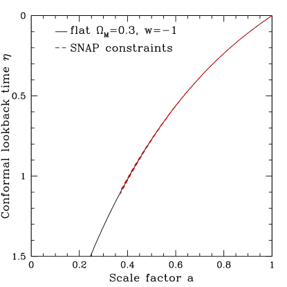
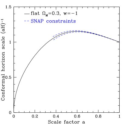
Figure 6: The expansion history is plotted in conformal time in the left figure. SNAP constraints appear very tight when viewed in conformal time because this is most closely related to the observations. The right figure shows the conformal horizon scale – the logarithmic derivative of the left figure. The part with negative slope allows comoving wavelengths to expand outside the horizon, or alternately represents $aH=\dot{a}$ increasing, i.e. $\ddot{a}>0$ – precisely the signature of inflation or acceleration. The dashed blue lines show that SNAP will map the accelerating phase, the transition, and into the matter dominated, decelerating phase of the past universe.

Figure 6 also shows the logarithmic derivative

$${d\eta\over d\ln a}=a{dt\over a\,da}=(\dot{a})^{-1}=(aH)^{-1},$$ (19)

interpreted respectively as the proper time evolution of the scale factor or the conformal horizon scale $(aH)^{-1}$. Just as in inflation a positive slope denotes decelerating expansion, $\ddot{a}<0$ and comoving wavelengths (e.g. of density perturbations) enter the horizon; v.v. for a negative slope: an accelerating universe or inflation. The dashed lines show that SNAP can probe both epochs and map the transition between them.

IV.5 Beyond Dark Energy

Mapping the physical time evolution of the scale factor relies on translating the observations into the behavior of the Hubble parameter $H(z)$. This translation might proceed via a parametrization of the physics of the acceleration, e.g. the dark energy properties as in §IV. We also might want to study the density evolution and its transition from the earlier matter dominated epoch to the present linexp . In §2 we adopted general relativity to obtain the Friedmann equation (4) to provide the foundation for these.

But ideally we would like to use the data to test the Friedmann equations of general relativity or alternate explanations for the acceleration besides dark energy. The supernova distance-redshift data allow such investigation of the fundamental framework by substituting the altered Hubble evolution $H(z)$ into Eq. (3). This enables constraints to be placed on, e.g., higher dimension theories, Chaplygin gas, etc. See Linder linexp for examples.

V Complementary Probes

In addition to the mapping of the expansion history through the distance-redshift relation by Type Ia supernovae or possibly other methods in the future, one can constrain the $a(t)$ curve in other ways. The total age of the universe places the “foot” of the $a(t)$ curve on the $a=0$ axis in the lower left of the plots. “Shooting upward” with a known slope ($a\sim t^{1/2}$ in the early radiation dominated epoch) provides a constraint on the $a(t)$ relation. Knox et al. knox have shown that the location of the acoustic peaks in the cosmic microwave background radiation power spectrum is nearly degenerate with the age in a flat universe not too different from ours. These data place a constraint of $t_{0}=14.0\pm 0.5$ billion years. The bounds in terms of $H_{0}t_{0}$ are slightly weaker because of increased model dependence: $0.93\pm 0.06$, $1.00\pm 0.07$ from supernovae saul ; h0t0 .

The $t$, as opposed to the $H_{0}t$, axis would thus have a stronger footpoint for the $a(t)$ curve to aim toward. But conversely, the slope of $a(t)$ near $a=1$ changes from unity on a $H_{0}t$ plot to the Hubble constant $H_{0}$ on a $t$ plot, adding another uncertainty. A direct bound on $H_{0}$ constrains the slope of the $a(t)$ curve at $a=1$ in the upper right of such plots. The Hubble Space Telescope Key Project freed quotes $H_{0}=72\pm 8$ km/s/Mpc. In either the $a-t$ or $a-H_{0}t$ plane constraints on present slope and total age together act to force the expansion history into a narrow corridor, shooting back in time subject to the boundary conditions.

VI Conclusion

The geometry, dynamics, and composition of the universe are intertwined through the theory of gravitation governing the expansion of the universe. By precision mapping of the recent expansion history we can hope to learn about all of these. The brightest hope for this in the near future is the next generation of distance-redshift measurements through Type Ia supernovae that will reach out to $z\approx 1.7$. This represents over 70% of the age of the universe and spans the current accleration epoch back to the matter dominated deceleration epoch when most large scale structure formed.

Just as the thermal history of the early universe taught us much about cosmology, astrophysics, and particle physics, so does the recent expansion history have the potential to greatly extend our physical understanding. With the new parametrization of dark energy suggested here, one can study the effects of a time varying equation of state component back to the decoupling epoch of the cosmic microwave background radiation. But even beyond dark energy, exploring the expansion history provides us cosmological information in a model independent way, allowing us to examine many new physical ideas. From two numbers we have progressed to mapping the entire dynamical function $a(t)$, on the brink of a deeper understanding of the dynamics of the universe.

References

- (1) A. Sandage, Ap.J. 133, 355 (1961)
- (2) S. Weinberg, Gravitation and Cosmology (Wiley, New York, 1972)
- (3) A. Sandage, Ann. Rev. A&A 26, 561 (1988)
- (4) E.V. Linder, A&A 206, 175 (1988)
- (5) E.V. Linder, First Principles of Cosmology (Addison-Wesley, London, 1997)
- (6) M. Tegmark, Science 296, 1427 (2002), astro-ph/0207199
- (7) E.W. Kolb and M.S. Turner, The Early Universe (Addison-Wesley, New York, 1990)
- (8) T. Banks and M. Dine, JHEP 0110, 012 (2001), hep-th/0106276
- (9) L.M. Krauss and G.D. Starkman, Ap.J. 531, 22 (2000), astro-ph/9902189
- (10) P. Steinhardt and N. Turok, astro-ph/0204479
- (11) SNAP (http://snap.lbl.gov) parameter error estimates are for 2000 SNe between and 300 SNe at from the Nearby Supernova Factory (http://snfactory.lbl.gov), plus a prior on of 0.03. Some numerical results were kindly provided by R. Miquel and N. Mostek; see Kim, Linder, Miquel & Mostek 2003, in preparation, for a description of the Monte Carlo fitter.
- (12) G.F.R. Ellis et al., Phys. Rep. 124, 315 (1985)
- (13) E.V. Linder, astro-ph/0108255
- (14) E.V. Linder and D. Huterer, submitted to Phys. Rev. D, astro-ph/0208138
- (15) P. Astier, astro-ph/0008306
- (16) D. Huterer and M.S. Turner, Phys. Rev. D 64, 123527 (2001), astro-ph/0012510
- (17) D. Huterer and G. Starkman, Phys. Rev. Lett. 90, 031301 (2003), astro-ph/0207517
- (18) J. Weller and A. Albrecht, Phys. Rev. D 65, 103512 (2002), astro-ph/0106079
- (19) P.S. Corasaniti and E.J. Copeland, to appear in Phys. Rev. D, astro-ph/0205544
- (20) E.V. Linder, in Proc. IDM2002, astro-ph/0210217
- (21) M. Chevallier and D. Polarski, Int. J. Mod. Phys. D 10, 213 (2001)
- (22) P. Brax and J. Martin, Phys. Lett. B 468, 40 (1999), astro-ph/9905040
- (23) Planck: http://astro.estec.esa.nl/Planck
- (24) J.A. Friemann, D. Huterer, E.V. Linder, and M.S. Turner, submitted to Phys. Rev. D, astro-ph/0208100
- (25) E.V. Linder, to appear in Phys. Rev. Lett., astro-ph/0208512
- (26) L. Knox, N. Christensen, and C. Skordis, Ap. J. Lett. 563, L95 (2001), astro-ph/0109232
- (27) S. Perlmutter et al., Ap. J. 517, 565 (1999), astro-ph/9812133
- (28) J.L. Tonry and the High-Z Supernova Search Team, in Astrophysical Ages and Time Scales, astro-ph/0105413
- (29) W. Freedman et al., Ap. J. 553, 47 (2001), astro-ph/0012376