Realistic error estimates on kinematic parameters

Abstract

Current error estimates on kinematic parameters are based on the assumption that the data points in the spectra follow a Poisson distribution. For realistic data that have undergone several steps in a reduction process, this is generally not the case. Neither is the noise distribution independent in adjacent pixels. Hence, the error estimates on the derived kinematic parameters will (in most cases) be smaller than the real errors. In this paper we propose a method that makes a diagnosis of the characteristics of the observed noise The method also offers the possibility to calculate more realistic error estimates on kinematic parameters. The method was tested on spectroscopic observations of NGC 3258. In this particular case, the realistic errors are almost a factor of 2 larger than the errors based on least squares statistics.

1 Introduction

The bulk of kinematic information available on elliptical galaxies is nowadays retrieved through observation and analysis of the line-of-sight velocity distributions (LOSVD’s) of the stars in these galaxies.

The basic idea behind the study of LOSVD’s is that a galaxy spectrum can be generated by the spectrum of a star of similar type that has been redshifted by the rotation of the galaxy and smeared out by the velocity dispersion of the stars (Minkowski, 1962).

The study of LOSVD’s as we know it now started about 30 years ago, when near the end of the seventies, Sargent et al, (1977) and Tonry & Davis, (1979) published surveys of galaxy redshifts and velocity distributions. The methods they presented in their papers were widely used afterward:

• Fourier quotient method (Sargent et al,, 1977): The LOSVD is obtained by dividing the Fourier transform of the galaxy spectrum by the Fourier transform of the template spectrum, and transform the result back into pixel space. Although it seems to be natural to use Fourier space, this has also some disadvantages. The error calculation becomes complicated due to the correlations in the quotient and the method is very sensitive to template mismatch.

• Cross-correlation method (Tonry & Davis,, 1979): The peak in the galaxy-template correlation function is fit by a Gaussian function. The method also provides a way to obtain error estimates on the kinematic parameters.

These techniques assume a Gaussian form for the broadening functions for mainly practical reasons: it provides a way of filtering the noise in the spectra and it allows to calculate convolutions analytically. The mean and variance determining the Gaussian function were considered as parameters describing the mean streaming and stellar velocity dispersion.

About ten to fifteen years later, the quality of the data had improved a lot and new techniques were developed trying to get more information out of the observed spectra than just two parameters. The main improvement was the elimination of the assumption of a Gaussian form for the LOSVD. There are mainly two criteria that can be used to classify these techniques: (a) whether a non-parametric LOSVD or a parameterized LOSVD is derived. In case of high S/N data, a non-parametric LOSVD yields all information you can get out of a spectrum. But because of the presence of noise there is always a need for some sort of smoothing. There are several ways to do this, either by adapting some filter or by using a smoothing parameter. For these non-parametric fitting methods there is not always a simple way to come to an error estimate. (b) whether the fit is performed in Fourier space or in pixel space. A treatment of the problem in pixel space has the advantage that parts of the spectrum can be easily eliminated and allows an easier error estimate.

A lot of methods have been proposed:

• Fourier fitting method (Franx et al.,, 1989): (parametric in Fourier space) A convolution of the LOSVD with the template is fitted to the galaxy spectrum in Fourier space. Error estimates are derived from a least squares fit.

• Fourier correlation quotient method (Bender,, 1990): (non-parametric in Fourier space) The method is based on the deconvolution of the peak of the template-galaxy correlation function with the peak of the autocorrelation of the template star. This approach is shown to be less sensitive to template mismatch than the standard Fourier quotient method. The deconvolution itself is done in Fourier space. Noise filtering is done by applying a Wiener filter. Error estimates can be retrieved from Monte Carlo simulations.

• Direct fitting method (Rix & White,, 1992): (non-parametric in pixel space) The galaxy spectrum is assumed to be a superposition of various components: (1) continuum terms, (2) a set of broadened stellar spectra where the broadening function and the stellar spectra can vary, (3) a noise component. The best combination of components and the errors on the results are obtained from a least squares minimization.

• unresolved Gaussian deconvolution (Kuijken & Merrifield,, 1993): (non-parametric in pixel space) The LOSVD is modeled as a sum of a set of Gaussian distributions that are uniformly spaced in velocity. The best fit is determined by means of a least square minimization, which also serves as basis for error determination.

• Bayesian method (Saha & Williams,, 1994): (non-parametric or parametric in pixel space) The concept is to take a trial LOSVD and convolve it with a template spectrum into a model spectrum. If this model is the real one, the difference between the model spectrum and the observed spectrum must be the noise. With probability theory it can be calculated what the probability is that the trial LOSVD is the true one, given the data. Confidence intervals for broadening functions are obtained from Monte Carlo simulations.

• Cross-correlation method update (Statler,, 1995): (parametric in pixel space) This is a generalization of the galaxy-template cross-correlation method to arbitrary parameterized line profiles, where the correlation function is fitted by the model line profile using a least squares technique. For a well resolved galaxy spectrum, the result is fairly insensitive to template mismatch. Errors follow out of standard statistics involved in the fitting technique.

• penalized likelihood (Merritt,, 1997): (non-parametric in pixel space) The method is based on a penalty function that is large for any noisy function and zero for a Gaussian function. This method allows to fit high quality data very accurately, whereas also very noisy data can be fitted, in the limit by a simple Gaussian. Monte Carlo simulations are performed to come to an error estimate.

When parameters based on the integrated moments of the LOSVD are sought for, one can also obtain these parameters in a one step process. In this case, a convolution of a parameterized expression for the LOSVD with a stellar template spectrum is matched to the observed galaxy spectrum.

• Gauss-Hermite fitting method (van der Marel & Franx,, 1993): (parametric in Fourier space) A Gauss-Hermite parameterization is used for the LOSVD, a least squares minimization is performed in Fourier space.

• Gauss-Hermite direct fitting method (van der Marel et al.,, 1994): (parametric in pixel space) The LOSVD is written as a truncated Gauss-Hermite series and the least squares fit is performed in pixel space.

It is generally believed that, if the data are good enough to apply non-parametric fitting, such an approach implies less bias than a parametric fit. However, having a non-parametric LOSVD, it is still very useful to describe the obtained profile by just a few characteristic numbers. Higher order information can be obtained either by calculating the moments of the velocity distribution or by fitting a parameterized function to it. Since there is a real danger of confusion when dealing with the moments of the LOSVD, we define them here explicitly:

$$\langle v_{p}\rangle=\int dv_{p}v_{p}{\cal L}(v_{p}),$$ (1)

and

$$\mu_{k}=\int dv_{p}(v_{p}-\langle v_{p}\rangle)^{k}{\cal L}(v_{p}),\quad k\neq 1,$$ (2)

with ${\cal L}(v_{p})$ the LOSVD. The kinematic moments are the mean projected rotation $\langle v_{p}\rangle$, the projected velocity dispersion $\sigma_{p}^{2}=\mu_{2}$, the skewness $\zeta_{3}=\mu_{3}/\sigma^{3}_{p}$ and the kurtosis $\zeta_{4}=\mu_{4}/\sigma^{4}_{p}$.

The calculation of higher order moments out of LOSVD’s may be troublesome because of the strong dependence of the moments on the wings of the profiles. These wings unfortunately are the hardest to retrieve from observations. Therefore, in most practical cases, a parameterized function is fitted to the LOSVD. A truncated Gauss-Hermite series is often used (Gerhard, 1993,van der Marel & Franx, 1993):

$${\cal L}(v_{p})=\gamma\exp\left[-{1\over 2}{(v_{p}-\langle v\rangle)^{2}\over\sigma^{2}}\right]\times\left[1+\sum_{j=3}^{n}h_{j}H_{j}\left({v_{p}-\langle v\rangle\over\sigma}\right)\right].$$ (3)

In this expression, $\langle v\rangle$ and $\sigma$ are free parameters, they are also called ’mean velocity’ and ’velocity dispersion’. The functions $H_{j}(x)$ are the $j$-th order Gauss-Hermite polynomials, and their coefficients $h_{j}$ are regarded as the higher order parameters. The coefficient $h_{3}$ is the third order shape parameter and is an indication for anti-symmetric deviations from a pure Gaussian function in the form of leading or trailing tails. The coefficient $h_{4}$ is the fourth order shape parameter and is an indication for symmetric deviations from a pure Gaussian LOSVD in the form of broader or smaller wings.

Kinematic information up (to parameters corresponding) to the fourth order moment of the LOSVD is becoming available for a large sample of ellipticals, see e.g Bender et al. (1994), Kronawitter et al., (2000), Halliday et al., (2001). These data sets are a prerequisite for the construction of dynamical models of elliptical galaxies. In some cases it can be noticed that the error estimates on the parameters are smaller than the scatter among neighbouring data points in the kinematic profiles. This is especially striking for the so-called higher order moments (third and fourth order moment). Examples of this behaviour can be seen in some of the data presented by Bender et al. (1994), Kronawitter et al., (2000), Halliday et al., (2001). A possible interpretation of this fact is that the real errors on the kinematic parameters are larger than the error estimates given by the parameter fitting algorithms.

The derivation of these error estimates relies on assumptions that are generally not completely met. Though people are aware of this, it is generally unclear how large the discrepancy between reality and assumptions is.

One can come up with at least two good reasons why it is important to have realistic error estimates for dynamical modelling. First, for the construction of dynamical models, it is convenient to work with a goodness of fit indicator, which is meant to be an objective indicator of how good the model fits the data. Such goodness of fit indicators need error estimates on the data. However, if these are not realistic errors, it is not straightforward to interpret the values of this goodness of fit indicator, let alone derive meaningful confidence intervals for the models. In some cases, awareness of this problem may prompt one to adopt modified error estimates for use in the goodness of fit indicator (e.g. Kochanek, (1994), Cretton et al. (2000), Gerhard et al., (1998), Saglia et al., (2000), Kronawitter et al., (2000)). However, playing with the error estimates on individual data points is equivalent to using different relative weights for the data points, and this is likely to complicate the interpretation of a goodness of fit indicator rather than simplify it.

A second issue of concern is that these parameters are often used to determine a realistic dynamical model and to constrain the potential of a galaxy at the same time. In particular the velocity dispersion and the fourth order parameter play an important role in inferring the existence of central black holes or dark matter haloes around elliptical galaxies. In practice this is done by assuming a potential for the system and trying to find a dynamical model based upon the selected potential that simultaneously fits the velocity dispersion and fourth order parameter within the given error estimates. If no such model can be found, it is concluded that the assumed potential is not the right one, and the amount of dark matter is changed. If the error estimates are smaller than the real errors and the conclusions on the potential critically depend on them (e.g. Rix et al., (1997), Kronawitter et al., (2000), Cretton & van den Bosch, (1999)), some potential-model combinations may be rejected wrongly. As an inevitable consequence, it is possible that in some cases the use of realistic error estimates in dynamical modelling will weaken the dynamical evidence for dark matter in elliptical galaxies.

The method to derive realistic error estimates on kinematic parameters that is presented in this paper reaches out toward a need on the observational side and the modelling side. The method makes an implicit diagnosis of the noise distribution and uses the characteristics of this distribution as the basis of a new error estimate.

In section 2, a diagnosis of the problem with error estimates is given. An outline of the new method is presented in section 3, this is elaborated and illustrated in section 4. A discussion and conclusions can be found in sections 5 and 6 respectively.

2 Diagnosis of the problem

In the absence of external sources of errors, a raw spectral image contains data points that follow a Poisson distribution, the variance of which is denoted by ”Poisson noise”. Another characteristic of a raw spectral image is that the data points in the image are independent. Hence, the power spectrum of the raw signal would match the definition of white noise: it has constant power in the frequency domain.

Before kinematic parameters can be calculated, the spectra have to be brought in a state that is referred to as ’cleaned’ and ’calibrated’. Bringing the spectra in such a condition requires a number of image processing steps, the so-called ’standard reduction techniques’, for which adequate tools are available in image analysis packages such as MIDAS or IRAF. But besides bringing the observed spectra in good condition, these reduction steps also have a non-negligible influence on the noise distribution.

For example, the removal of bad pixels or cosmic ray events, where the values of two or more adjacent pixels are replaced by an average over a surrounding region, clearly introduce dependencies in the data. Likewise, dependencies are introduced by any operation where some kind of interpolation is involved, like e.g. calibration. Moreover, a sky subtraction does certainly not guarantee a perfect elimination of the sky in the data, regardless the level of sophistication that is used to perform the operation. The residual of this correction also adds up to the noise distribution. In some cases the above effects can be the source of considerable uncertainties on the derived kinematic parameters, while this is not reflected by error estimates based on Poisson noise.

In many cases, a least squares technique is used to derive the kinematic parameters and error estimates from the data. The statistical interpretation of this method relies on the assumption that (1) the noise is independent and (2) Gaussian distributed on the input data. For large numbers, a Gaussian distribution is a fairly good approximation for a Poisson distribution and therefore the second assumption is valid. It is clear from the above arguments that the first condition generally is not met after data reduction. As a consequence, the errors derived from standard statistics will in many cases differ from the real errors on the kinematic parameters.

Sometimes, Monte Carlo simulations are used (Bender et al. (1994), Statler, (1995)) to estimate the uncertainties on the derived parameters. For the realization of synthetic galaxy spectra, a Gaussian noise distribution with given S/N is used. So also this method may show a similar tendency to underestimate the errors.

Accepting the fact that the cleaned and calibrated spectral images come as they are, it is possible to obtain error estimates that are more realistic estimates than those currently found in literature. This is the purpose of the present paper.

3 Outline of the method

To get an idea of more realistic errors on the parameters and to overcome the above problems we propose the following scheme. The steps are described in more detail in the following sections.

• Perform a fit of a model galaxy spectrum to the observed galaxy spectrum and determine the residual of this fit. The model galaxy spectrum is a convolution of the selected template spectrum with a LOSVD. For this step it is important to use an expression for the LOSVD that offers enough freedom. The purpose is to fit every part of the galaxy spectrum that can reasonably be fit by a convolution of the template spectrum with a general and smooth LOSVD.

• The residual of this fit contains (1) the Gaussian noise on the raw spectrum, (2) the features left or introduced by several reduction steps. The errors estimated with the proposed method take into account artifacts from flatfielding, cosmic remnants, effects of rebinning and remnants of sky removal, for as far as the latter has been removed reasonably well. On the other hand, the method does not account for errors in continuum subtraction nor template mismatch. Hence, the residual of the fit can be considered as a realization of the ”observed noise” involved in the problem: the term ”observed noise” applies to ’cleaned and calibrated’ spectra and is used to make a distinction with Poisson noise. Where pure white noise is featureless and transforms into a flat power spectrum, the power spectrum of the residual will be different. A smooth representation of the power spectrum of the residual will be taken as sufficient information on the main characteristics of the observed noise.

• The next step is to generate a number of synthetic galaxy spectra, that have a noise distribution with the same power spectrum as the observed noise, and to use these synthetic spectra to determine the spread on the kinematic parameters. These equivalent noise distributions that carry the characteristics of the original observed noise can be obtained by multiplying the Fourier transform of a white noise profile with a smooth representation of the power spectrum of the residual, and transforming this back.

The idea of using Monte Carlo simulations to determine error estimates of course is not new, but the main point is that in the present method one tries to model the real characteristics of the noise.

A demonstration of the method on realistic galaxy spectra is given in section 4.

4 NGC 3258

4.1 Observations

NGC 3258 is an E1 galaxy and was observed with the ESO-NTT telescope in the nights of 27-28/2/2001 (64.N-192). Spectra of the major axis were taken using the red arm of EMMI, covering the Ca II triplet. Grating #7 was used, having a dispersion of 0.66 Å/pix. The detector was a Tektronix CCD with 2048$\times$2047 pixels, 24$\mu m\times$24$\mu m$ in size and with a pixel scale of $0.27^{\prime\prime}$/pixel. A slit width of $1.5^{\prime\prime}$ thus yields a spectral resolution of 3.67 Å FWHM, resulting in an instrumental dispersion of about 54 km/s in the region of the Ca II triplet. For NGC 3258, several exposures of 3600 sec were taken (in total 11 hours). A number of standard stars (G dwarfs and K and M giants) were also observed.

4.1.1 Standard data reduction steps

Standard reduction steps were applied to these spectra. Out of the bias and dark exposures a correction term was derived. Several domeflat images were used to come to an appropriate flatfield image. Cosmics were removed using a top hat filter. After filtering, the images were inspected carefully and remaining cosmics were also removed by hand.

For the wavelength calibration, lamp spectra were taken just before or after each of the spectroscopic observations of the galaxy or the stellar template stars. For each row in the lamp spectra images, a polynomial was constructed to transform the pixel scale into wavelength scale. The same coordinate transformation was then applied to the galaxy or star spectra. The calibrated images have a step of $0.3$Å.

For the airmass correction, the mean value of the airmass at the beginning and end of the exposure was used. The contribution of the sky to the spectra was estimated from an upper and lower region of the image, where there was no contribution of the light of the galaxy or template star. Several galaxy spectra were reduced separately, aligned and combined into one galaxy spectra image.

Spatial rebinning of the galaxy spectra resulted in data with a S/N $\geq$ 50/bin (about 70 in the centre). Only a small part of the spectrum, from 8500 Å to 8750 Å was used to determine the kinematic parameters.

4.2 The observed noise on the data

The idea is that the residual of the observed galaxy spectrum with a sufficiently flexible model spectrum can be attributed to some sort of noise involved in the problem. For a given stellar template spectrum it is important to consider a representation for the LOSVD that offers enough degrees of freedom to be able to find the best fitting model spectrum.

For this reason, nonparametric LOSVD’s in combination with a flexible method to generate them are chosen to perform this fit. We have also chosen not to restrict ourselves to positive LOSVDs, because this makes the fit more general and at this point there are no physical restrictions on the LOSVDs. The method adopted here performs a least squares fit, using a set of cubic spline basis functions to represent the LOSVD. An outline of the method can be found in Appendix A. However, for this step, any non-parametric fitting method with enough degrees of freedom will do. The model spectrum was a linear combination of convolutions with a number of observed template stars in which the coefficients were chosen on the basis of a goodness of fit estimator.

The non-parametric fit is only used to get an idea of the fraction of the signal in the galaxy spectrum that cannot be accounted for by a model spectrum with the chosen template mix, and hence that will be part of the residual. Furthermore, also traces of sky lines, or incompletely removed cosmics will contribute to the residual of this fit.

Figure 1: At position $r=0.8^{\prime\prime}$: the galaxy spectrum and non-parametric fit in the middle panel and the residual of the fit in the lower panel. The upper panel shows the LOSVD resulting from the non-parametric fit.

Figure 2: At position $r=11^{\prime\prime}$: the galaxy spectrum and non-parametric fit in the middle panel and the residual of the fit in the lower panel. The upper panel shows the LOSVD resulting from the non-parametric fit.

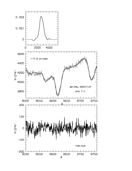
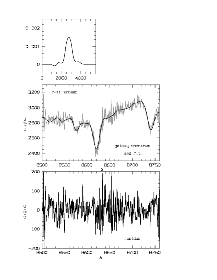
As an illustration, the results of the method for two different positions along the major axis of NGC 3258 are shown in figure 1 for $r=0.8^{\prime\prime}$ and figure 2 for $r=11^{\prime\prime}$. The upper panel displays the LOSVD, obtained from a non-parametric fit with 10 degrees of freedom. The middle panel shows the observed galaxy spectrum and the fit. The lower panel shows the residual of the fit. From these lower panels is it clear that the residual at $11^{\prime\prime}$ (values mostly between -100 and 100) is much larger than the residual at $0.8^{\prime\prime}$ (values mostly between -60 and 60). This immediately shows that the Poisson noise is not the only source of errors. The galaxy spectrum at $0.8^{\prime\prime}$ has much more counts in absolute value than the galaxy spectrum at $11^{\prime\prime}$, hence pure Poisson noise is higher at $0.8^{\prime\prime}$ than at $11^{\prime\prime}$. The surplus non-Poissonian contribution to the residual at $11^{\prime\prime}$ is likely to come mostly from an imperfect sky subtraction.

4.3 The power spectrum of the residual

Figure 3: The power spectrum of the noise involved in the fit (black line) and white noise (gray line). The smoothed observed noise profile is shown in black dashed line, the constant level of the white noise is shown in gray dashed line. Upper panel: at position $r=0.8^{\prime\prime}$. Lower panel: at position $r=11^{\prime\prime}$.

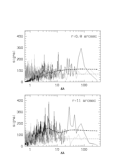
To see what the magnitudes of the various frequency components in these residuals are, their power spectra have been calculated. They are presented in figure 3, the residual at $0.8^{\prime\prime}$ is in the upper panel, the residual at $11^{\prime\prime}$ in the lower panel. The scale on the horizontal axis is the period of the power spectrum, instead of the more widely used frequency. This period (labelled $\Delta\lambda$) is directly related to the wavelength scales of the features in the original spectrum. Because of the wide range in values for $\Delta\lambda$, a logarithmic axis is plotted. On top of the residual power spectra in figure 3, a sample power spectrum for the expected white noise at these radii is presented. There is a clear difference between both profiles.

Having these power spectra representations, one would like to know which part is playing an important role for the determination of real errors on the kinematics. In other words, which frequencies can have an important impact on the derived kinematic parameters?

Figure 4: The shaded regions show the regions of influence of injected wave functions with different wavelengths on the measurement of kinematic parameters.

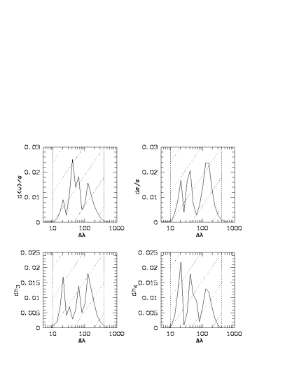
This can be investigated by means of some simulations. Galaxy spectra with various noise characteristics can be created starting from a galaxy spectrum obtained after convolution of a template spectrum with a known LOSVD and adding wave functions (sine and cosine functions) with different frequencies. For these artificial spectra, a best fitting model spectrum was determined using a least-squares minimization. The model spectrum was composed with the template spectrum and a LOSVD expressed as a truncated Gauss-Hermite series. This analysis of the artificial spectra gives new values for the kinematic parameters, that will differ from the original kinematic parameters. The results of such simulations as a function of the scale size of the waves can be seen in figure 4 (upper panels for d$\langle v\rangle$/$\sigma$ and d$\sigma$/$\sigma$, lower panels for d$h_{3}$ and d$h_{4}$).

It is clear that the measurement of these kinematic parameters is sensitive to superpositions of wave functions with wavelengths ($\Delta\lambda$) between 10 Å and 400 Å (hashed regions in figure 4). This $\Delta\lambda$ range is independent of the wavelength range used in the analysis, but scales with $\sigma$ (which is 325 km/s in this case).

This learns that the region of interest in the power spectrum of the residuals lies between $\Delta\lambda=10$Å and $\Delta\lambda=400$Å. It is also there (see figure 3) that the residual power spectra overshoot the white noise.

For short wavelengths, the residual power spectrum seems to have lower values than the Poisson noise power spectrum. At first sight this seems to be puzzling. However, this is a result of the interpolations that took place in the course of the data reduction process. Interpolation always implies some sort of smoothing, which means that features with a small wavelength scale disappear from the image.

Moreover, oversampling lies at the origin of the transfer of an amount of noise coming from small wavelength scale to larger wavelength scale. The stronger the oversampling, which has the artificially enlarging of feature wavelength scales as a result, the stronger this migration effect. In the case of NGC 3258, the original spectrum had a step of $0.66$Å/pixel, while the spectra after calibration have a step of $0.3$Å/pixel.

4.4 Realistic error estimates

The power spectra of the residuals clearly show that the assumption of independent (white) noise is not a valid one. This implies that the classical statistical tools for calculating error estimates out of least squares fitting techniques cannot be used.

The only option that is left, is to determine the uncertainties on the parameters through Monte Carlo simulations. In this case it is important to work with simulated galaxy spectra that have the same noise characteristics as the original galaxy spectrum. Our method proposes to achieve this by using simulated galaxy spectra that give residuals that follow the same power spectrum as the initially determined residual.

To realize this, a smooth representation of the residual power spectrum is created. This is illustrated in figure 3, by means of the dashed lines. In this case, each pixel was replaced by a weighted mean over 20 pixels at each side taking a linearly declining weight function into account. This smooth function has basically the same behaviour as the power spectrum, and hence carries the information that distinguishes the observed noise distribution from white noise. New realizations of this noise distribution can be calculated by multiplying a white noise spectrum with this fitted function. In this way, the simulated galaxy spectra for the Monte Carlo simulation are constructed.

To these spectra, a model spectrum composed with the template spectrum and a parameterized expression for the LOSVD is fitted. For the parameterization, a Gauss-Hermite decomposition was used, following van der Marel & Franx, (1993). The best fitting values for $\langle v\rangle$, $\sigma$, $h_{3}$ and $h_{4}$ were obtained using the Levenberg-Marquardt method as described in Press et al., (1989).

Figure 5: Kinematic parameters for NGC 3258. The realistic error estimates are shown by means of vertical lines, the horizontal lines on these error estimates indicate an estimate for the errors based on least squares statistics.

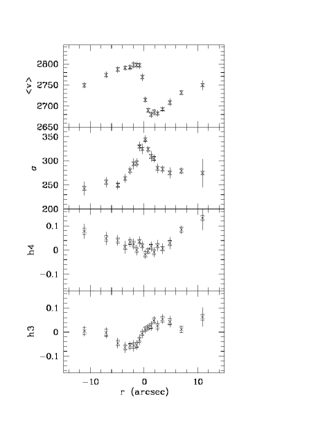
The error estimates are the root mean squares of the kinematic parameters that were derived from 100 realizations of the galaxy spectra. The results are shown in figure 5, from upper to lower panel: the mean rotation velocity, the velocity dispersion, $h_{4}$ and $h_{3}$. The vertical error estimates present realistic errors. The horizontal lines correspond to error estimates based on least squares statistics.

The mean velocity reaches a maximum value of about 56 km/s and the realistic error estimates lie between 5.7 km/s and 11.3 km/s (with a mean error of 7.5 km/s and a mean error from least squares statistics of 4 km/s). The central velocity dispersion is 344 km/s, with an error of 8 km/s. The mean error on $\sigma$ is 10.4 km/s, the mean error on $\sigma$ based on least squares statistics is 3.8 km/s. For large radii, the profile is antisymmetric.

The profile for $h_{3}$ goes through the origin, apparently there is no serious problem with template mismatch. The mean error on $h_{3}$ is 0.02, the lowest value is about 0.013, the highest value is 0.039 (measured in an outer point). From least squares statistics, the mean error on $h_{3}$ is 0.01.

The $h_{4}$ profile is approximately symmetric, with low values in the centre and higher values for the outer data points. The central data points show quite some scatter, but this is not inconsistent with the errors (at least 0.014) on the data in that region. The errors increase outwards, the outer data points have an error of 0.049 (positive side) and 0.03 (negative side). The mean error on $h_{4}$ is 0.023, the mean error on $h_{4}$ following least squares statistics is 0.01.

For the $h_{3}$ and $h_{4}$ profiles, we compared the data points at either side of the centre. The amount of scatter in the profiles can be expressed as the mean distance between corresponding data points at positive and negative radius, $\sqrt{(\sum_{i=1,n}(|y_{i}|-|y^{\prime}_{i}|)^{2})/n}$, with $n$ the number of data points at positive or negative radius, and $y_{i}$ and $y^{\prime}_{i}$ the values for the parameters in corresponding points at positive and negative side of the centre. Fore $h_{3}$ the value of this scatter indicator is 0.019 and for $h_{4}$ this is 0.031. This means that for both parameters, the mean errors derived with the proposed method are close to this scatter indicator, while the mean errors following from least squares statistics are clearly smaller.

5 Discussion

To verify and validate the algorithm and its implementation, we now explore a few situations in which (following the discussion in section 2) conventional and more realistic error bars based on the method described in this paper are expected to give different results by means of simulations. Using simulations has the advantage that also the true errors can be calculated and hence the error estimates can be compared.

5.1 Impulse noise

A fraction of the noise with non-Poissonian character is manifested as spikes that overshoot the Poisson noise and that are relatively small on wavelength scale. This situation can be mimicked in a simulation by adding impulse noise to a spectrum with otherwise pure Poisson noise.

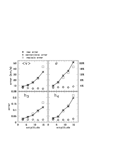
Synthetic model spectra were obtained by convolving a LOSVD characterized by $\langle v\rangle=h_{3}=h_{4}=0$ and $\sigma=250$ km/s with a K3 giant and adding Poisson noise. Different types of model spectra were then created by contaminating 10 $\%$ of the pixels in the spectrum with impulse noise with an amplitude of 3, 6, 9, 12 or 15 times the amplitude of the Poisson noise.

The RMS deviation on the kinematic parameters calculated out of 100 equivalent realization of one type of synthetic spectrum are considered to be the true errors on the kinematic parameters in that specific situation. For each type of spectrum, also the analyses following the scheme outlined in section 3 was applied (these results will be referred to as realistic errors). Likewise, conventional errors were calculated with a standard least squares technique. These results are presented in figure 6. The true errors are indicated in asterisks, the realistic errors in squares and the conventional errors in diamonds.

It is clear that the conventional errors returned by a standard technique are independent of the degree of contamination and can underestimate the true errors considerably. For an impulse noise with an amplitude of 3 times that of the Poisson noise the conventional error underestimates the true error by $\sim 27\%$ for $\langle v\rangle$, $\sim 37\%$ for $\sigma$, $\sim 31\%$ for $h_{3}$ and $\sim 35\%$ for $h_{4}$. The realistic errors on the other hand follow the true errors much better. For the same situation the difference between realistic errors and true errors is $\sim 10\%$ for $\langle v\rangle$, $\sim 5\%$ for $\sigma$, $\sim 0\%$ for $h_{3}$ and $\sim 14\%$ for $h_{4}$. For serious contamination, with an impulse noise with an amplitude of 15 times that of the Poisson noise, the realistic error bars seem to slightly overestimate the real errors, but this is hopefully no longer a realistic situation.

Figure 6: Results of a simulation where impulse noise is added to a spectrum with pure Poisson noise. The amplitude of the impulse noise, relative to the amplitude of the Poisson noise is indicated on the horizontal axis. On the vertical axis are the measured errors. The asterisks indicate the true errors on the kinematic parameters, the squares indicate the realistic errors and the diamonds indicate the conventional errors.

5.2 Sampling

Changing the original sampling step of a spectrum has an impact on the error propagation that is completely neglected when Poisson noise is used as basic assumption for the error calculation.

For the simulations, a number of synthetic spectra were obtained with the same LOSVD and template star as above, but the number of pixels was different for each spectrum. In the end, all synthetic spectra were resampled in order to end up with spectra with $N$ pixels. This means that for the final spectra, the wavelength scale was $n$ times the original wavelength scale, with $n$ equal to 1.5, 2, 3 or 4, in order to mimic oversampling, and also $n$ equal to 0.5 and 0.25, thus mimicking undersampling.

These sampling factors are chosen only for the sake of illustrating the method. These rebinned spectra were analysed using the technique described in section 3, yielding realistic errors, and using a standard technique for the conventional errors. Again, the real errors were calculated out of Monte Carlo simulations with 100 spectra. The resulting error estimates are presented in figure 7, in squares for the realistic errors and diamonds for the conventional errors. The true errors are indicated in asterisks. Again, the conventional errors are independent of any change in amount of over- or undersampling, while the realistic errors mainly follow the true errors. The change in errors scales roughly with $\sqrt{n}$, with $n$ the sampling factor.

Figure 7: The results of simulations with rebinned spectra, where the wavelength scale after rebinning is $n$ times the wavelength scale of the original spectrum. The sampling factor $n$ is on the horizontal axis, the vertical axes represents the errors. The true errors are indicated in asterisks, the realistic errors in squares and the conventional error in diamonds.

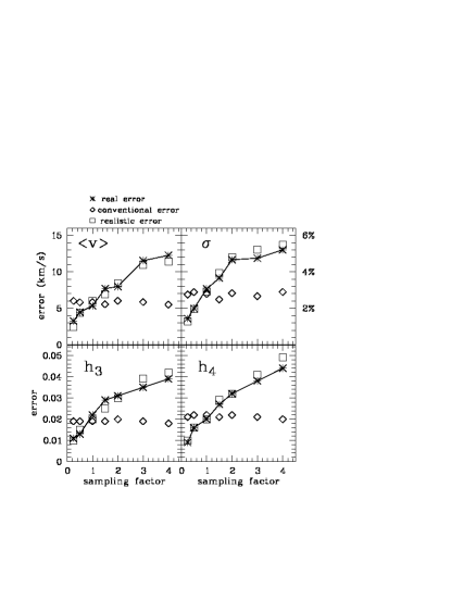
This result shows that care should be taken if kinematic parameters and conventional errors are estimated from spectra that are logarithmically rebinned. In that case the wavelength scale is clearly changed, but in such a way that some regions are more compressed and other regions are stretched.

5.3 Template mismatch

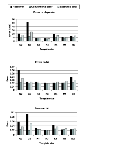
We do not claim that the proposed method is able to cope with the errors coming from template mismatch. But also in this case, the errors estimated with the method presented in this paper are closer to the true errors than the conventional errors obtained by standard techniques. The synthetic spectrum, created with a K3 giant, was also analysed with the following templates: G2 dwarf, G5 dwarf, K1 giant, K4 giant, M1 giant, M2 giant. The results are presented in figure 8. The horizontal axis shows the sequence of template stars, the bars indicate the errors: black for the true error, dark gray for the conventional error and light gray for the realistic error (indicating that the error is obtained using the technique presented in this paper). The results for $\sigma$ are in the upper panel, the results for $h_{3}$ in the middle panel and the results for $h_{4}$ in the lower panel. The results for $\langle v\rangle$ are not shown because the correction for the radial velocity of the template star would introduce an additional uncertainty.

It is clear that the true errors (black bars) are larger than the conventional errors and the realistic errors. For all three kinematic parameters, it is remarkable that the conventional errors show little variation if different stellar templates are used, whereas the differences in values for the ”realistic” errors are larger. Moreover, in cases with large true errors, the ”realistic” errors are closer to these values than the conventional errors. It seems that the errors obtained with this method can be used as indicators for template mismatch in the sense that larger errors indicate a poorer fitting template, whereas the conventional errors clearly cannot be used as such.

Figure 8: The results of simulations with other templates. The horizontal axis shows the sequence of template stars, the bars indicate the errors: black for the true error, dark gray for the conventional error and light gray for the ”realistic” error using this technique. The results for $\sigma$ are in the upper panel, the results for $h_{3}$ in the middle panel and the results for $h_{4}$ in the lower panel.

6 Conclusions

As the technical limitations on the quality of observed data are diminishing, the numerical signal processing starts putting limitations on the information content of the observations. Therefore, it is important to have realistic estimates of the errors on the data.

In this paper, we propose a new method to calculate error estimates on kinematic parameters derived from spectroscopic observations. The starting point is the realization that the data points in the ’reduced and calibrated’ spectral images do not follow a Poisson distribution and are not independent from pixel to pixel. This implies that the error estimates derived with classical tools (Monte Carlo simulations with Gaussian noise or statistical interpretation of least squares techniques) will underestimate the true errors in many cases.

The proposed method first determines the characteristics of the real noise on the data. For this, a flexible fitting method offering enough degrees of freedom is used. The residual of the fit is considered as observed noise. It is shown that the power spectrum of this observed noise can be very different from white noise. Realistic error estimates are obtained through Monte Carlo simulations with synthetic galaxy spectra, where the noise distribution follows the same power spectrum as the observed noise. In this way, errors are estimated taking the real characteristics of the noise into account, instead of relying on a Gaussian (or Poisson) noise distribution. Moreover, the proposed scheme can be applied in combination with several methods that are currently used to derive kinematic parameters from spectroscopic data.

The method was tested on spectroscopic observations of NGC 3258. In this particular case, the realistic errors are almost a factor of 2 larger than the errors based on least squares statistics. What is most important, is that the realistic error estimates are more consistent with the scatter among neighbouring data points in the kinematic profiles.

Simulations with spectra containing Poisson noise and impulse noise confirm that the proposed method offers error estimates that are closer to the true errors than conventional error estimates. Moreover, from simulations with synthetic spectra it becomes clear that an oversampling of the spectra results in an underestimate of the errors on kinematic parameters when simple least squares statistics are used. This may be an important consideration when kinematic parameters are calculated from logarithmically rebinned spectra. Although this method is not able to calculate realistic errors on kinematic parameters obtained with an ill matching template star, the realistic errors do trace the situation of template mismatch, in the sense that they become larger with increasing template mismatch, unlike the usual error estimates.

Appendix A Cubic spline fit

Figure 9: Left: A first type of third degree cubic spline, composed with the functions I and II. Right: A second type of third degree cubic spline, composed with the functions III and IV. The definitions can be found in the text.

In this paper, a new method is used to perform a non-parametric fit of a model spectrum to an observed galaxy spectrum. The method performs a least squares fit, using a set of cubic spline basis functions to represent the LOSVD.

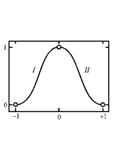
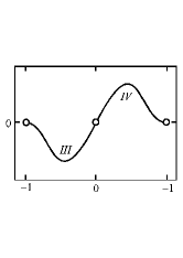
Each basis function is a third-degree cubic spline. There are two types of cubic spline basis functions, each a composition of two polynomials, as illustrated in figure 9.

In this figure, the cubic splines are defined in the interval [-1,1]. The first third degree basis function (left in figure 9) is a composition of polynomials I and II. The second basis function (right in figure 9) is a composition of polynomials III and IV. These polynomials are:

$$I = 1-3x^{2}-2x^{3}=(1+x)^{2}(1-2x)$$ (4)

$$II = 1-3x^{2}+2x^{3}=(1-x)^{2}(1+2x)$$ (5)

$$III = x+2x^{2}+x^{3}=(1+x)^{2}x$$ (6)

$$IV = x-2x^{2}+x^{3}=-(1-x)^{2}x$$ (7)

Function I is defined in the interval [0,1] and meets the requirements that $y(1)=0=y^{\prime}(1)$, $y(0)=1$, $y^{\prime}(0)=0$, (prime denoting first order derivative). This behaviour is mirrored with respect to the vertical axis into the region [-1,0], resulting in function II. The composition of I and II gives a symmetric cubic spline basis function. The first two conditions assure that the function declines smoothly to 0 at the edges. The other two conditions give the profile a flat peak on the y-axis.

Function IV is defined in the interval [0,1] and meets the requirements that $y(1)=0=y^{\prime}(1)$, $y(0)=0$, $y^{\prime}(0)=1$. This behaviour is mirrored with respect to the centre into the region [-1,0], resulting in function III. The composition of III and IV is an antisymmetric cubic spline basis function. Again, the first two conditions assure that the function declines smoothly to 0 at the edges. The other conditions make sure the function goes through the centre and give a steeply declining or inclining profile near the centre.

Figure 10: Implementation scheme for the non-parametric fit. The fitting interval is divided in a number of sub-intervals. Every two adjacent sub-intervals are used to define a set of cubic splines that is included in the fit. This means that four basis functions of different type (I, II, III, IV) are defined in each sub-interval.

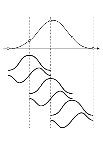
For the practical implementation, the interval where the fit is performed is divided in $(n-1)$ sub-intervals, using $p_{i}$, $i=1,\ldots,n$ points. This is illustrated in figure 10. Each triplet of adjacent points $p_{i-1},p_{i},p_{i+1}$ is used to define a set of cubic splines that is included in the fit.

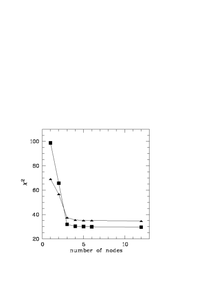
The choice of the number of sub-intervals or basis functions is free. The less sub-intervals are considered, the more the line profile is smoothed. There is no a priori criterion that can be used to decide how many of these sub-intervals have to be used to obtain a good fit. Instead, a number of fits with an increasing number of sub-intervals (hence basis functions) is performed and the $\chi^{2}$ values of the fits then indicate when the number of cubic spline pairs offers enough degrees of freedom to come to a good fit. This is illustrated in figure 11; once a sufficient degree of freedom is reached, the values for $\chi^{2}$ start decreasing only very slowly when the number of nodes is increased. If $n$ points are used, $(n-1)$ sub-intervals are used for the fit, yielding $2n-4$ degrees of freedom.

Figure 11: The $\chi^{2}$ values of a number of fits with an increasing number of sub-intervals, for the spectra at $r=0.8^{\prime\prime}$ (filled squares) and $r=11^{\prime\prime}$ (filled triangles). For both spectra, using four nodes or more gives about the same values for $\chi^{2}$.

Kuijken & Merrifield (1993) came up with a similar idea, but they used Gaussian functions for the decomposition of the LOSVD. The cubic splines used here are for the same degrees of freedom slightly more flexible in fitting. The fit is not restricted to strictly positive results. If one wants to obtain physical solutions with this method, linear constraints can be added to the $\chi^{2}$ fit.

References

- Bender, (1990) Bender R., 1990, A&A, 229, 441
- Bender et al. (1994) Bender R., Saglia R.P., Gerhard O.E., 1994, MNRAS, 269, 785
- Cretton et al. (2000) Cretton N., Rix H.W., de Zeeuw P.T., 2000, ApJ, 536, 319
- Cretton & van den Bosch, (1999) Cretton N., van den Bosch F.C., 1999, ApJ, 514, 704
- Franx et al., (1989) Franx M., Illingworth G., Heckman T., 1989, ApJ, 344, 613
- Gerhard, (1993) Gerhard O.E., 1993, MNRAS, 265, 213
- Gerhard et al., (1998) Gerhard O.E., Jeske G., Saglia R.P., Bender R., 1998, MNRAS, 295, 197
- Halliday et al., (2001) Halliday C., Davies R.L., Kuntschner H., Birkinshaw M., Bender R., Saglia R.P., Baggley G., 2001, MNRAS, 326, 473
- Kochanek, (1994) Kochanek C.S., 1994, ApJ, 436, 56
- Kronawitter et al., (2000) Kronawitter A., Saglia R.P., Gerhard O., Bender R., 2000, A&AS, 144, 53
- Kuijken & Merrifield, (1993) Kuijken K., Merrifield M.R., 1993, MNRAS, 264, 712
- Merritt, (1997) Merritt D., 1997, AJ, 114, 228
- Minkowski, (1962) Minkowski R., 1962, Problems of Extragalactic Research, Ed. G.C. McVittie, Macmillan, New York, p. 112
- Press et al., (1989) William H. Press, Saul A. Teukolsky, William T. Vetterling, and Brian Flannery, Cambridge University Press, 702 pp. 1989
- Rix & White, (1992) Rix H.W., White S., 1992, MNRAS, 254, 389
- Rix et al., (1997) Rix H.W., de Zeeuw P.T., Cretton N., van der Marel R., Carollo M., 1997, ApJ, 488, 702
- Saglia et al., (2000) Saglia R.P., Kronawitter A., Gerhard O., Bender R., 2000, AJ, 119,153
- Saha & Williams, (1994) Saha P., Williams T.B., 1994, AJ, 107, 1295
- Sargent et al, (1977) Sargent W. L. W., Schechter P. L., Boksenberg A., Shortridge K., 1977, ApJ, 212, 326
- Simkin, (1974) Simkin s., 1974, A&A, 31, 129
- Statler, (1995) Statler T.S., 1995, AJ, 109, 1371
- Tonry & Davis, (1979) Tonry J., Davis M., 1979, AJ, 84, 1511
- van der Marel & Franx, (1993) van der Marel R.P., Franx M., 1993, ApJ, 407, 525
- van der Marel et al., (1994) van der Marel R. P., Rix H. W., Carter D., Franx M., White S. D. M., de Zeeuw T, 1994, MNRAS, 268, 521