The Stellar Content of M31’s Bulge11affiliation: Based on observations with the NASA/ESA Hubble Space Telescope obtained at the Space Telescope Science Institute, which is operated by AURA for NASA under contract NAS5-26555.
Abstract
In this paper we analyze the stellar populations present in M31 using nine sets of adjacent HST-NICMOS Camera 1 and 2 fields with galactocentric distances ranging from to . These infrared observations provide some of the highest spatial resolution measurements of M31 to date; our data place tight constraints on the maximum luminosities of stars in the bulge of M31. The tip of the red giant branch is clearly visible at , and the tip of the asymptotic giant branch (AGB) extends to . This AGB peak luminosity is significantly fainter than previously claimed; through direct comparisons and simulations we show that previous measurements were affected by image blending. We do observe field-to-field variations in the luminosity functions, but simulations show that these differences can be produced by blending in the higher surface brightness fields. We conclude that the red giant branch of the bulge of M31 is not measurably different from that of the Milky Way’s bulge. We also find an unusually high number of bright blueish stars (7.3 arcmin-2) which appear to be Galactic foreground stars.
1 Introduction
The first deep infrared (IR) observations of stars in the bulge of our Galaxy were carried out by Frogel & Whitford (1987). Measuring the luminosity function (LF) using the M giant grism surveys of Blanco, McCarthy & Blanco (1984) and Blanco (1986), they found many luminous giants, but noticed that the LF has a sharp break at (), with the brightest stars extending to .
The tip of red giant branch (RGB), defined by the core mass required for helium flash, occurs at a luminosity of . Any stars brighter than this limit are therefore on the asymptotic giant branch (AGB). The stars observed in the Galactic bulge extend magnitudes brighter than the tip of the RGB. Since metal-poor ([Fe/H]) Galactic globular clusters do not exhibit such luminous AGB stars, this might have suggested a younger age for the bulge population, since the luminosity of the brightest AGB stars increases with decreasing age (e.g. Iben & Renzini, 1983). However metal-rich globular clusters do have stars which can reach luminosities of , while still having ages comparable to the metal poor clusters (Frogel & Elias, 1988; Guarnieri, Renzini & Ortolani, 1997). Moreover, it has been demonstrated that the stellar population of the Galactic bulge is dominated by metal-rich stars ([Fe/H]) (McWilliam & Rich, 1994) that are as old as Galactic globular clusters (Ortolani et al., 1995; Feltzing & Gilmore, 2000; Kuijken & Rich, 2002; Zoccali et al., 2002), and that the number of stars brighter than the RGB tip is consistent with the frequency observed in old, metal rich globular clusters. In summary, the stellar population in the bulge of the Milky Way is as old as the oldest Galactic globular clusters, and old, metal rich stellar populations are able to produce AGB stars only as bright as .
Work was already underway studying stars in other nearby galaxies to determine whether the properties of the stars in the Galactic bulge are typical of all bulges. The nearest and brightest large spiral, M31 (the Andromeda Galaxy) was the obvious first choice for a comparison. Some of the first measurements of stars in the inner bulge of M31 ( kpc from the nucleus) were made by Mould (1986). He found that M31’s brightest bulge stars were magnitude more luminous than the brightest stars in M31’s halo. Rich et al. (1989) then took spectra of some of these bright stars, and found most to have properties characteristic of late-type M giants.
It was unclear what was causing the apparent difference between the stellar populations of the bulges of the Milky Way and M31. The dependence of the AGB peak luminosity on mass (and therefore age and mass loss) and metallicity pointed to several possible explanations for this observed difference. However, all of these explanations implied a difference in the formation or evolutionary processes of these two otherwise very similar galaxies.
To see if the luminous stars in M31 are indeed similar to those found in the bulge of the Milky Way, Rich & Mould (1991) measured a sample of stars in the inner bulge of M31 from the nucleus with the Hale 5m reflector (see §8.2). Their resulting LF had a drop at , similar to that seen in BW, but extended to . To explain these excess luminous stars they proposed several theories. (1) These stars could be younger stars from the disk superposed on the bulge. (2) They could be super-metal-rich in chemical composition, since the luminosity of the brightest AGB stars increases with metallicity. (3) The bulge of M31 could have a young stellar component, since the luminosity of the brightest AGB stars increases with decreasing age (Iben & Renzini, 1983). (4) They could be the result of merged lower-mass main-sequence stars (blue straggler progenitors), which produces more massive and luminous stars.
Soon thereafter, Davies, Frogel & Terndrup (1991) imaged the M31 bulge in the near-IR using the 3.8m UKIRT facility, albeit from the nucleus, a factor of two more distant than Rich. Their LF has an upper limit mag brighter than that seen in the Galactic bulge. They argued that contamination by stars from a young disk, which lies behind the bulge, is most likely responsible for the luminous stars observed by RM91.
DePoy et al. (1993) carried out a -band survey of stars in 604 arcmin2 of Baade’s Window to check the possibility that the M giant surveys in the bulge of the MW (Blanco, McCarthy & Blanco, 1984; Blanco, 1986) may have missed very luminous stars similar to the ones seen in the bulge of M31. The DePoy et al. (1993) observations turned up no such population of luminous stars, and their derived LF is consistent with that obtained by Frogel & Whitford (1987). In order to compare their Galactic Bulge observations with those of the bulge of M31, DePoy et al. (1993) rebinned and smoothed their image to simulate the M31 observations. The resulting degraded image showed that few if any of the “stars” on this simulated M31 field corresponded to individual stars on the original image; most were just random groupings of stars. A quantitative analysis showed that the extreme crowding caused an artificial brightening in the LF of more than one magnitude. They thus concluded that the luminous stars seen in M31’s bulge were most likely not real, but an artifact of image crowding.
At nearly the same time Rich, Mould & Graham (1993) acquired new observations of five fields in the bulge of M31 with the Palomar IR Imager on the Hale 5m telescope (see §8.1). By measuring the LFs in fields with different expected disk contributions from 2 to 11 arcminutes from the nucleus, they rejected the hypothesis of Davies, Frogel & Terndrup (1991) that the bright stars are disk contaminants. Using their own model fields, which showed that they could accurately measure the GB tip despite the crowding, they also argued against the idea of DePoy et al. (1993) that the bright stars are stellar blends. While they did concede that some of their measurements may have been affected by crowding of up to 1 magnitude, they maintained that they were not generally measuring clusters of blended images. Further calculations by Rich, Mould & Graham (1993) also showed the numbers of blue straggler progeny stars to be insufficient to explain the number of luminous stars.
In pursuit of a resolution to this controversy, Rich & Mighell (1995) obtained HST Wide-Field Planetary Camera (WFPC1) observations of the inner bulge of M31. Regretfully, these observations were taken with HST’s original aberrated optics, reducing the effective resolution to barely better than was available from the ground. These observations also yielded many luminous stars, although not quite as bright as previously measured. The data also suggested that the brightest stars may be concentrated toward the center of M31.
Approaching this problem from the theoretical side, Renzini (1993, 1998) performed calculations to estimate the number of stars in all evolutionary stages in each pixel. He showed that the number of blends increases quadratically with both the surface brightness of the target and with the angular resolution of the observations. Applying these calculations to existing photometric data for the inner bulge of M31, he concluded that all previous ground-based observations were dominated by blends, and even questioned the HST observations of Rich & Mighell (1995), pointing to the measured blue colors as indicative of their blended origin.
With the Wide-Field Planetary Camera 2 (WFPC2), Jablonka et al. (1999) observed three fields in the bulge of M31 at optical wavelengths. With HST’s improved resolution, they did not find stars more luminous than those in the Galactic Bulge, and concluded that previous detections of very bright stars were likely the result of blended stars due to the crowding in WFPC1 and ground-based images.
However, since even very luminous evolved stars can go undetected at optical wavelengths due to molecular blanketing, Davidge (2001) recently obtained new infrared images of the bulge of M31 with the 3.6m CFHT. With the help of adaptive optics (AO), his observations confirm the optical non-detection of very luminous stars made by Jablonka et al. (1999). Although there is agreement between the brightest stars measured by (Davidge, 2001) in the bulge of M31 and the brightest stars measured in the Galactic Bulge (Frogel & Whitford, 1987), the luminosity functions still show considerable differences. The M31 bulge LF measured by Davidge (2001, Figure 7) does not show a break at as is observed in BW, but instead shows a change in slope at and a break at , indicative of different star formation histories in the MW and M31 if correct.
Thus it appears that this decade-old controversy has not yet been completely resolved. While there now appears to be agreement that the brightest of the previous measurements were blends, it is still not certain whether the luminosity functions of the bulges of the Milky Way and M31 are consistent with one another. In this paper we will show that indeed they are, and that even the most recent observations, including our own, are still affected by blending in the inner regions of M31.
The layout of the paper is as follows. We start by describing our observations in Section 2, and our reduction and photometric techniques in Section 3. We present the color magnitude diagrams and luminosity functions in Sections 4 and 5 respectively. Section 6 gives a brief theoretical analysis of blending in M31, followed by detailed simulations of all our fields in Section 7. In Section 8 we compare our measurements with previous observations; Rich, Mould & Graham (1993) in §8.1, Rich & Mould (1991) in §8.2, and Davidge (2001) in §8.3. Section 9 discusses the bright stars which appear to be Galactic foreground stars, and we conclude with a brief summary of our results in Section 10.
2 Observations
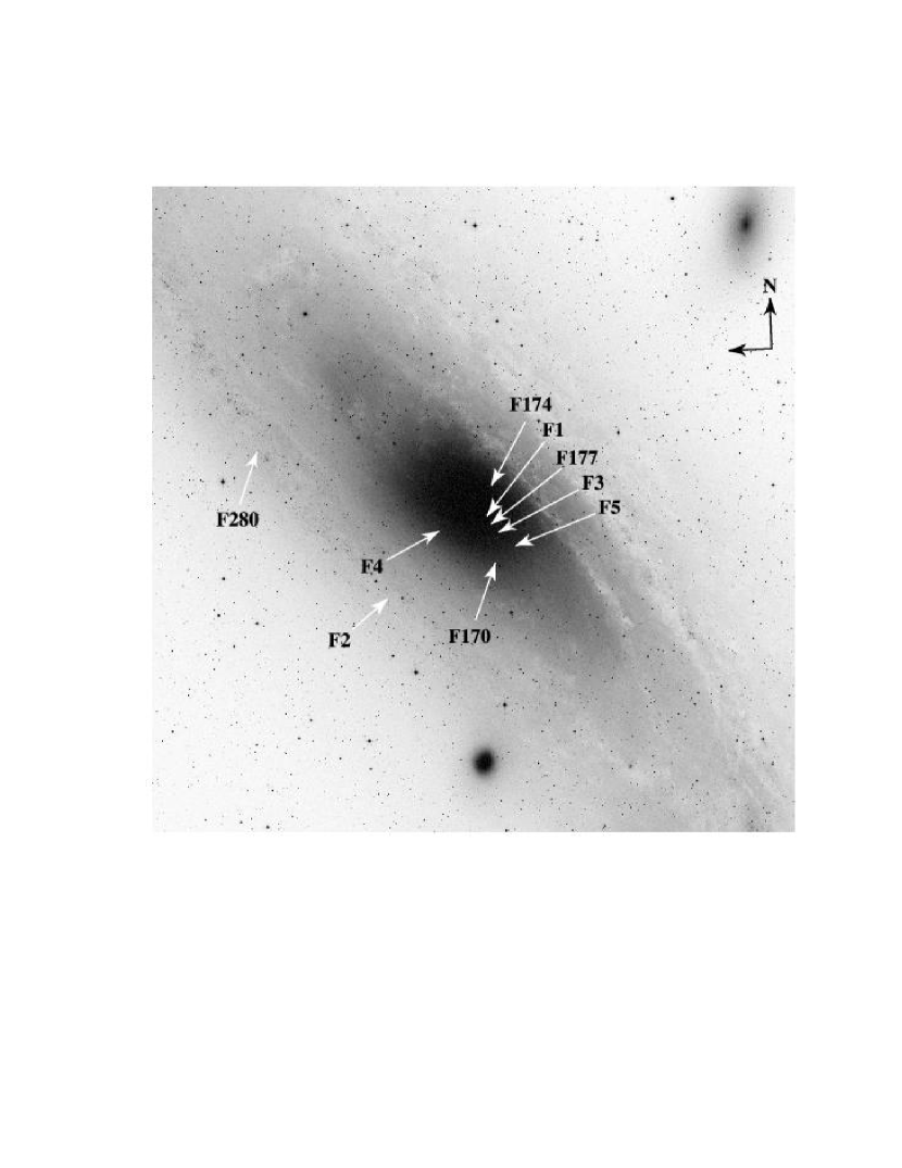
In this paper we analyze images of M31 taken from two different NICMOS proposals. Proposal 7876 imaged the five central fields of Rich, Mould & Graham (1993). These fields were carefully chosen to sample varying bulge/disk ratios, and are indicated by F1–F5 on Figure 1. Proposal 7826 imaged five globular clusters in M31. The four fields used in this study are indicated on Figure 1 by their cluster numbers: F170, F174, F177 and F280. We omit the G1 field from this analysis, since at 34 kpc from the center of M31, the frame is dominated by cluster stars.
Since the NIC1 and NIC2 cameras are at different positions in the HST focal plane, we can simultaneously image 2 fields at each pointing (see Figure 2). The NIC2 field is across, and separated by from the NIC1 field ( between field centers). Their different sizes are due to their different spatial resolutions; the NIC1 images have a plate scale of pixel-1, compared to the pixel-1 of NIC2. Having different resolutions at each pointing will prove useful for understanding the severe crowding very near the center of M31.

Our observations are summarized in Table 1. The top half of the table lists our NIC1 observations, and the second half is for NIC2. The first column lists the field ID; the second and third give the field coordinates. The distance from the center of M31 in arcminutes is listed in column 4. Using this distance, the position angle from the major axis of M31, the -band surface brightness from Kent (1989), and an assumed color of 2.9, we estimate the -band surface brightness of each field, which is listed in column 5. Taking Kent’s bulge – disk decomposition, we also give the bulge/disk ratio in column 6.
| ID | aaJ2000 | aaJ2000 | Radius | bbmag/arcsec-2, from Kent (1989) assuming . | Bulge/Disk |
|---|---|---|---|---|---|
| (1) | (2) | (3) | (4) | (5) | (6) |
| NIC1 | |||||
| F1 | 0h42m3783 | 41° | 15.09 | 6.4 | |
| F2 | 0h43m2846 | 41° | 18.72 | 0.1 | |
| F3 | 0h42m3263 | 41° | 15.91 | 3.5 | |
| F4 | 0h43m213 | 41° | 16.88 | 1.3 | |
| F5 | 0h42m2551 | 41° | 16.37 | 2.1 | |
| F170 | 0h42m3214 | 41° | 16.68 | 1.7 | |
| F174 | 0h42m3315 | 41° | 15.52 | 4.9 | |
| F177 | 0h42m3530 | 41° | 15.58 | 4.7 | |
| F280 | 0h44m3063 | 41° | 18.35 | 0.2 | |
| NIC2 | |||||
| F1 | 0h42m3630 | 41° | 14.98 | 7.7 | |
| F2 | 0h43m2707 | 41° | 18.54 | 0.1 | |
| F3 | 0h42m3087 | 41° | 15.82 | 3.9 | |
| F4 | 0h43m044 | 41° | 16.57 | 1.9 | |
| F5 | 0h42m2263 | 41° | 16.40 | 2.0 | |
| F170 | 0h42m3240 | 41° | 16.52 | 1.9 | |
| F174 | 0h42m3330 | 41° | 15.78 | 4.1 | |
| F177 | 0h42m3440 | 41° | 15.40 | 5.5 | |
| F280 | 0h44m2950 | 41° | 18.33 | 0.2 |
The NICMOS focus was set at the compromise position 1-2. This is the best focus for simultaneous observations with cameras 1 and 2. All of our observations used the multiaccum mode (MacKenty et al., 1997) because of its optimization of the detector’s dynamic range and cosmic ray rejection.
Our primary (pointed) observations were taken with NIC2. Each field was observed through three filters: F110W (0.8–1.4 µm), F160W (1.4–1.8 µm), and F222M (2.15–2.30 µm). These filters are close to the standard ground-based , , & filters. However, to maximize the depth of our parallel NIC1 observations, we only used the F110W () filter. Total integration times and FWHMs for each camera and filter combination are given in Table 2. The dates of the observations are listed in Table 3.
All the observations implemented a spiral dither pattern with 4 positions to compensate for imperfections in the infrared array. For fields F1–F5 the dither steps were for the and band images, and for the band images. Fields F170–F280 are the same, except that we used dithers in .
As previously mentioned, the observations of fields F170–F280 are from another proposal targeting M31’s metal-rich globular clusters (Stephens et al., 2001b). In these observations we exclude stars inside radii of , , , and around the clusters G170, G174, G177 and G280 respectively, to avoid cluster stars.
| NIC1 | NIC2 | |||
|---|---|---|---|---|
| Fields | F110W | F110W | F160W | F222M |
| F1–F5 | 4992 | 1280 | 2048 | 1664 |
| F170–F280 | 7552 | 1920 | 3328 | 2304 |
| FWHM | ||||
| Field | Date |
|---|---|
| F1 | 1998/09/20 |
| F2 | 1998/09/18 |
| F3 | 1998/09/24 |
| F4 | 1998/09/23 |
| F5 | 1998/10/13 |
| F170 | 1998/08/10 |
| F174 | 1998/08/13 |
| F177 | 1998/09/08 |
| F280 | 1998/09/13 |
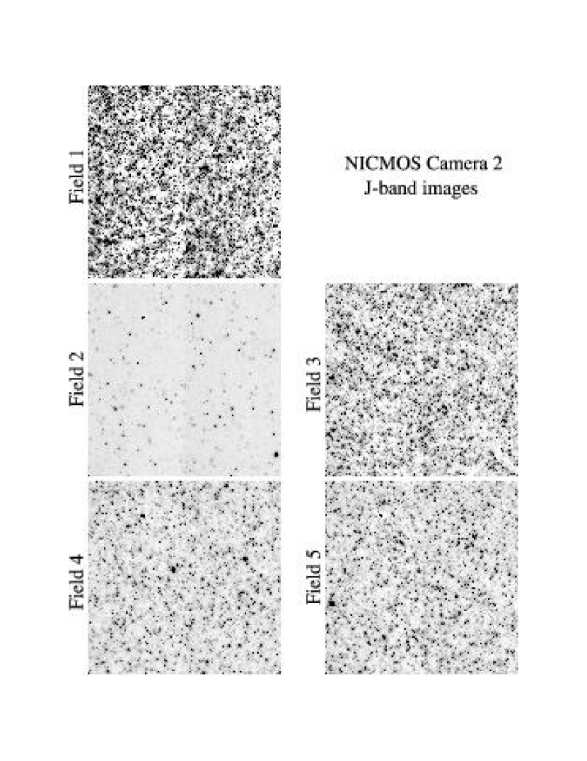
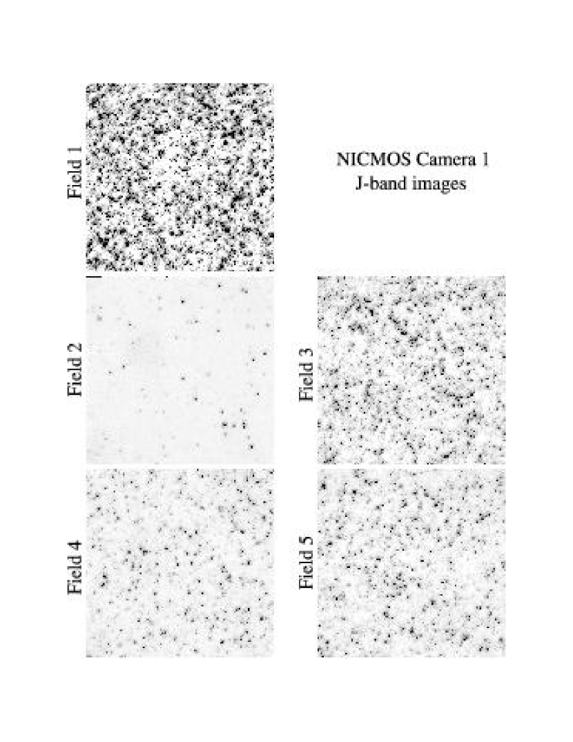
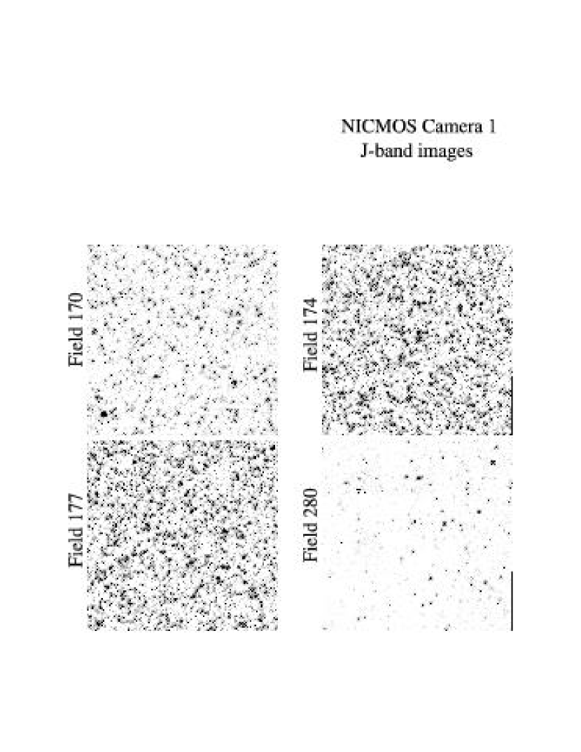
Images of fields F1-F5 are shown in Figures 3 and 4 for NIC2 and NIC1 respectively. The NIC1 images of fields F170-F280 are shown in Figure 5, and their NIC2 counterparts are given in Figure 2 of Stephens et al. (2001b). These images are the combination of 4 and 12 dithers for NIC2 and NIC1 respectively. The dimensions of each set of combined images are different due to the varying plate scale and dither size, and are given in the figure captions.
When converting to absolute or bolometric magnitudes we assume a distance modulus to M31 of , which corresponds to 3.7 parsecs arcsec-1, and an extinction of .
3 Data Reduction & Photometry
Our data were reduced with the STScI pipeline supplemented by the Image Reduction and Analysis Facility (IRAF 111IRAF is distributed by the National Optical Astronomy Observatories, which are operated by AURA, Inc., under cooperative agreement with the NSF.) nicproto package (May 1999) to eliminate any residual bias (the “pedestal” effect). Object detection was performed on a combined image made up of all the dithers of all the bands (12 images in total). Point spread functions (PSFs) were determined from each of the four dithers, then averaged together to create a single PSF for each band of each target. Instrumental magnitudes were measured using the allframe PSF fitting software package (Stetson, 1994), which simultaneously fits PSFs to all stars on all dithers. daogrow (Stetson, 1990) was then used to determine the best magnitude in a radius aperture.
We finally transformed our photometry to the CIT/CTIO system. The NIC2 measurements used the transformation equations of Stephens et al. (2000), listed in equations 1-3. The NIC1 transformation proved to be more complicated, and is based on a comparison with the much lower spatial resolution groundbased observations of Rich, Mould & Graham (1993). A detailed description of the technique is given in Appendix A.
The selection criteria are also slightly different for stars measured in the NIC1 and NIC2 fields. For the NIC2 frames we require measurements in all three bands, with PSF-fitting errors smaller than 0.25 magnitudes in each band. For NIC1, with only -band observations, we only require that the PSF-fitting error be less than 0.25 magnitudes.
| (1) | |||
| (2) | |||
| (3) |
4 Color-Magnitude Diagrams
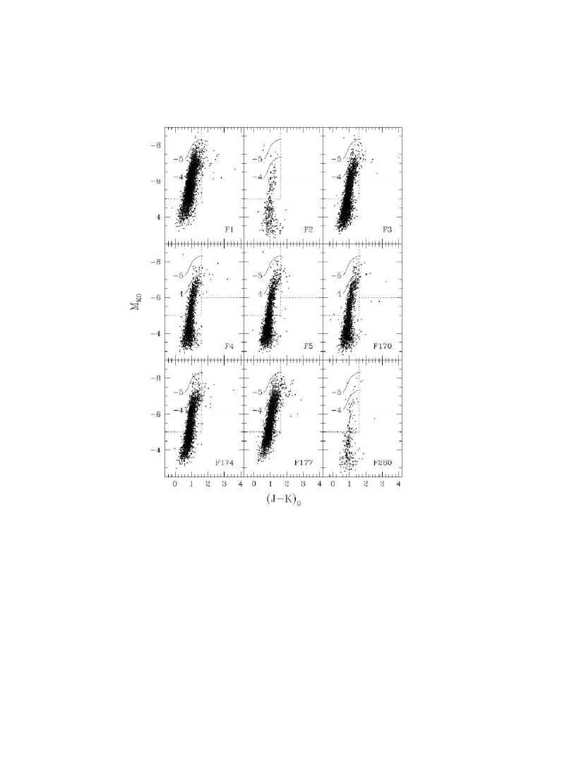
The – color-magnitude diagrams of all 9 NIC2 fields are shown in Figure 6. The overplotted solid lines are contours of constant bolometric magnitudes of and , based on the bolometric corrections for M giants in Baade’s Window calculated by Frogel & Whitford (1987). These plots assume a distance modulus to M31 of , , and .
The RGB and AGB are both visible in these CMDs. The tip of the RGB is more clearly defined in the less crowded fields, and a differential bolometric LF shows that it occurs at . In the more crowded fields the RGB tip gets blurred because of blending, which pushes stars up off of the RGB. The tip of the bulge AGB extends to . This AGB tip is significantly fainter than previously claimed, and we address this in a comparison with previous observations in Section 8.
4.1 LPVs
Long-period variables (LPVs) are large amplitude, luminous red variable stars with periods ranging from 50 to several hundred days. These stars are on the AGB and represent the brief final stages of low- to intermediate-mass stellar evolution on the giant branch. Based on measurements of variables in the Galactic Bulge (Frogel & Whitford, 1987), we have marked the region of each CMD where we expect to find primarily LPVs (Fig. 6). This region is indicated by a dashed box in the upper right of each CMD, with and . Since image blending generally shifts objects to bluer colors (Stephens et al., 2001a), this region should be relatively insensitive to crowding causing spurious LPV candidates, although in extreme cases, LPVs may actually be shifted blueward out of the box, thus only giving us a lower limit to the number of LPVs. A casual comparison of this LPV region between fields shows that some of the CMDs, particularly from the inner fields, have many more potential LPVs.
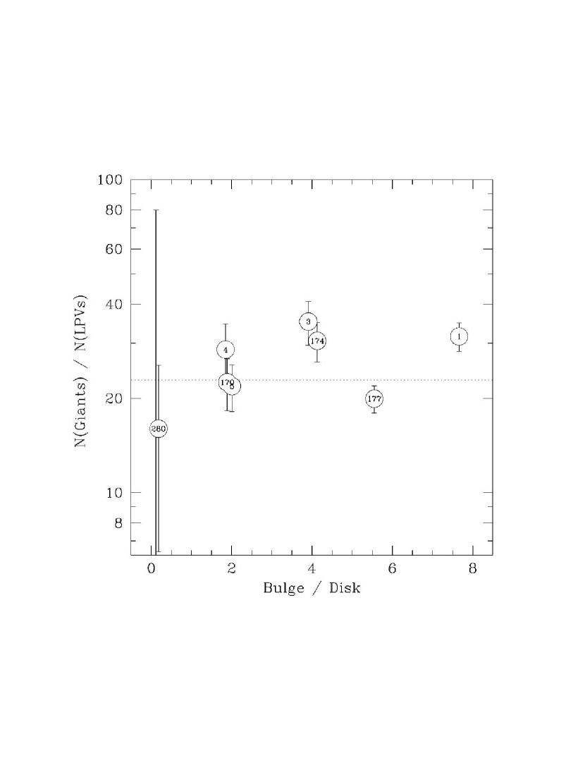
Since the relative numbers and luminosities of LPVs are sensitive to the age and/or metallicity of the parent population, LPVs can be used to look for field-to-field variations in the stellar population. Frogel & Whitelock (1998) argue that the relative number of LPVs to non-variable giants is independent of [Fe/H] for [Fe/H], and for higher metallicities the LPV lifetime is significantly reduced due to increased mass loss rates. Thus for stellar systems with a super-solar metallicity component, the ratio of non-variables to LPVs will appear high compared to lower metallicity systems. This idea seems to be supported by their determination of a higher non-variable giants to LPV ratio in the Galactic bulge compared to globular clusters.
To determine whether there is a change in the relative numbers of LPV candidates among our fields, we compare their numbers to the number of nonvariable giants, classified by having and . The ratio of giants to LPVs for each of our NIC2 fields is shown in Figure 7 as a function of bulge/disk ratio. This plot shows no trend in the giant/LPV ratio, instead all of our observations are scattered around the average ratio of N(Giants)/N(LPVs). Thus the LPVs appear to be uniformly distributed with the nonvariable stars.
5 Luminosity Functions
The -band LFs measured in all 18 fields are shown in Figure 8 and listed in Table 4 in units of number per magnitude per square arcsecond. The figure shows both the NIC1 and NIC2 LFs overplotted for each field. The first thing to note about this compilation of M31 LFs is that the NIC1 and NIC2 measurements are not exactly the same. While most show good agreement, several of the NIC2 LFs extend to brighter magnitudes, and all of the NIC1 LFs extend fainter.
The faint end differences are a combined result of the longer exposure times and better spatial resolution of NIC1. The NIC1 exposure times are nearly four times longer than those of the -band NIC2 observations. This is because while NIC2 was cycling through all three , & filters, NIC1 observed only through the -band filter. The faint end photometry is also affected by the level of crowding in the field. NIC2 is undersampled at , making it more difficult to distinguish close objects. Thus in very crowded fields, NIC1 has an advantage over NIC2, accounting for the larger faint-end difference seen in the more crowded fields.
There are several reasons for the differences seen at the bright end. The first is the difference in the field of view of each camera. NIC2 covers an area on the sky three times that of NIC1, and thus has a much better chance of finding the rarer brighter stars. Second is resolution and image sampling. NIC1 has a well sampled -band PSF with a FWHM of , while the NIC2 -band PSF is undersampled with a larger FWHM of . Also, the NIC2 photometric calibration requires detections in all three bands. Thus the limiting resolution for NIC2 is actually the -band, which has a FWHM of , nearly twice the size of the NIC1 -band PSF. The combined result is that the NIC2 observations are more sensitive to blending, which can artificially brighten stars, extending the bright end of the LF. Finally, there is the coincidence that most of the NIC1 observations occur in regions of slightly fainter surface brightnesses than their NIC2 counterparts (see Table 1 and Figure 2), somewhat exacerbating both aforementioned effects.
The -band NIC2 LFs are shown in Figure 9 and listed in Table 5, both normalized to give number/arcsec2/magnitude. Although NIC1 is more resilient against blending, both NIC1 and NIC2 observations are susceptible to its ill effects (see §7). However, under the hypothesis that all the measured bulge LFs arise from a single true LF, and that the differences are purely a result of blending, we estimate that the tip of the AGB occurs at and .


| NIC1 | NIC2 | |||||||||||||||||
|---|---|---|---|---|---|---|---|---|---|---|---|---|---|---|---|---|---|---|
| F1 | F2 | F3 | F4 | F5 | F170 | F174 | F177 | F280 | F1 | F2 | F3 | F4 | F5 | F170 | F174 | F177 | F280 | |
| 15.875 | 0.00 | 0.00 | 0.00 | 0.00 | 0.00 | 0.00 | 0.00 | 0.00 | 0.00 | 0.00 | 0.00 | 0.00 | 0.01 | 0.00 | 0.00 | 0.00 | 0.00 | 0.00 |
| 16.125 | 0.00 | 0.00 | 0.00 | 0.00 | 0.00 | 0.00 | 0.00 | 0.00 | 0.00 | 0.00 | 0.00 | 0.00 | 0.00 | 0.00 | 0.00 | 0.00 | 0.00 | 0.00 |
| 16.375 | 0.00 | 0.00 | 0.00 | 0.00 | 0.00 | 0.02 | 0.00 | 0.00 | 0.00 | 0.00 | 0.00 | 0.00 | 0.00 | 0.00 | 0.00 | 0.00 | 0.00 | 0.00 |
| 16.625 | 0.00 | 0.00 | 0.00 | 0.00 | 0.00 | 0.00 | 0.00 | 0.00 | 0.00 | 0.00 | 0.00 | 0.00 | 0.01 | 0.01 | 0.00 | 0.00 | 0.00 | 0.00 |
| 16.875 | 0.00 | 0.00 | 0.00 | 0.00 | 0.00 | 0.00 | 0.00 | 0.00 | 0.00 | 0.00 | 0.00 | 0.01 | 0.00 | 0.00 | 0.00 | 0.00 | 0.00 | 0.00 |
| 17.125 | 0.00 | 0.00 | 0.00 | 0.00 | 0.00 | 0.02 | 0.00 | 0.00 | 0.00 | 0.01 | 0.01 | 0.00 | 0.00 | 0.00 | 0.00 | 0.00 | 0.00 | 0.00 |
| 17.375 | 0.00 | 0.00 | 0.00 | 0.00 | 0.00 | 0.00 | 0.00 | 0.02 | 0.00 | 0.02 | 0.01 | 0.01 | 0.00 | 0.00 | 0.00 | 0.01 | 0.00 | 0.00 |
| 17.625 | 0.03 | 0.00 | 0.00 | 0.00 | 0.00 | 0.00 | 0.00 | 0.02 | 0.00 | 0.02 | 0.00 | 0.02 | 0.00 | 0.00 | 0.00 | 0.03 | 0.03 | 0.01 |
| 17.875 | 0.11 | 0.00 | 0.00 | 0.00 | 0.00 | 0.02 | 0.02 | 0.06 | 0.02 | 0.16 | 0.00 | 0.02 | 0.02 | 0.05 | 0.02 | 0.09 | 0.12 | 0.00 |
| 18.125 | 0.11 | 0.03 | 0.06 | 0.00 | 0.03 | 0.03 | 0.17 | 0.16 | 0.05 | 0.48 | 0.01 | 0.15 | 0.02 | 0.06 | 0.06 | 0.08 | 0.17 | 0.01 |
| 18.375 | 0.19 | 0.00 | 0.06 | 0.11 | 0.03 | 0.08 | 0.20 | 0.12 | 0.02 | 1.01 | 0.01 | 0.17 | 0.07 | 0.08 | 0.11 | 0.18 | 0.52 | 0.06 |
| 18.625 | 0.92 | 0.03 | 0.19 | 0.00 | 0.17 | 0.09 | 0.39 | 0.39 | 0.02 | 1.70 | 0.03 | 0.38 | 0.08 | 0.25 | 0.11 | 0.56 | 0.76 | 0.03 |
| 18.875 | 2.36 | 0.00 | 0.22 | 0.36 | 0.14 | 0.22 | 0.89 | 0.70 | 0.02 | 3.95 | 0.02 | 0.92 | 0.39 | 0.50 | 0.37 | 1.34 | 2.00 | 0.01 |
| 19.125 | 4.14 | 0.11 | 1.11 | 0.36 | 1.08 | 0.59 | 2.59 | 2.31 | 0.05 | 4.90 | 0.08 | 1.79 | 0.81 | 1.04 | 0.81 | 2.28 | 3.01 | 0.12 |
| 19.375 | 5.81 | 0.03 | 2.33 | 0.72 | 0.94 | 0.91 | 3.14 | 3.30 | 0.14 | 5.33 | 0.11 | 2.39 | 1.04 | 1.32 | 1.01 | 2.71 | 3.45 | 0.09 |
| 19.625 | 6.00 | 0.22 | 2.72 | 1.47 | 1.72 | 1.05 | 4.14 | 3.86 | 0.09 | 5.12 | 0.08 | 2.83 | 1.41 | 1.50 | 1.19 | 2.86 | 4.13 | 0.06 |
| 19.875 | 7.08 | 0.14 | 2.89 | 1.22 | 1.58 | 1.27 | 3.67 | 4.16 | 0.14 | 5.31 | 0.19 | 2.67 | 1.27 | 1.42 | 1.57 | 2.76 | 3.80 | 0.13 |
| 20.125 | 7.69 | 0.25 | 3.39 | 1.22 | 1.92 | 0.98 | 4.33 | 4.89 | 0.19 | 5.24 | 0.24 | 3.00 | 1.60 | 1.69 | 1.25 | 3.23 | 4.19 | 0.10 |
| 20.375 | 9.33 | 0.03 | 3.61 | 1.42 | 1.50 | 1.66 | 5.52 | 5.47 | 0.23 | 4.44 | 0.18 | 3.59 | 1.68 | 1.87 | 1.66 | 3.48 | 4.05 | 0.16 |
| 20.625 | 10.28 | 0.14 | 4.86 | 1.75 | 2.33 | 1.61 | 5.91 | 6.00 | 0.17 | 3.61 | 0.17 | 4.03 | 2.14 | 2.29 | 1.69 | 3.48 | 3.90 | 0.19 |
| 20.875 | 11.36 | 0.19 | 4.78 | 2.06 | 3.31 | 2.33 | 7.69 | 6.67 | 0.34 | 2.25 | 0.33 | 4.35 | 2.41 | 3.10 | 2.30 | 3.78 | 3.31 | 0.27 |
| 21.125 | 12.50 | 0.36 | 6.25 | 2.17 | 3.97 | 2.56 | 8.77 | 8.34 | 0.33 | 1.19 | 0.34 | 3.97 | 2.68 | 3.12 | 2.65 | 2.90 | 1.76 | 0.41 |
| 21.375 | 12.53 | 0.44 | 7.61 | 3.17 | 4.58 | 3.33 | 8.50 | 8.62 | 0.48 | 0.51 | 0.37 | 2.74 | 2.75 | 2.79 | 2.66 | 2.21 | 0.88 | 0.30 |
| 21.625 | 9.58 | 0.50 | 9.25 | 4.06 | 5.94 | 3.58 | 7.88 | 8.36 | 0.67 | 0.17 | 0.30 | 1.60 | 2.35 | 2.29 | 2.39 | 0.70 | 0.27 | 0.45 |
| 21.875 | 6.36 | 0.42 | 10.56 | 5.03 | 6.83 | 4.59 | 5.41 | 5.19 | 0.56 | 0.06 | 0.35 | 0.48 | 1.58 | 1.44 | 1.69 | 0.25 | 0.05 | 0.41 |
| 22.125 | 3.00 | 0.94 | 8.89 | 6.08 | 7.47 | 3.69 | 3.12 | 3.48 | 0.64 | 0.00 | 0.28 | 0.11 | 0.68 | 0.44 | 0.78 | 0.06 | 0.01 | 0.41 |
| 22.375 | 1.69 | 1.00 | 6.69 | 6.14 | 6.28 | 2.44 | 1.69 | 1.97 | 1.12 | 0.00 | 0.19 | 0.00 | 0.19 | 0.16 | 0.34 | 0.01 | 0.00 | 0.20 |
| 22.625 | 0.47 | 1.03 | 4.36 | 6.72 | 5.36 | 1.28 | 0.89 | 1.09 | 0.97 | 0.00 | 0.14 | 0.00 | 0.08 | 0.03 | 0.09 | 0.00 | 0.00 | 0.22 |
| 22.875 | 0.36 | 1.06 | 2.69 | 5.78 | 4.28 | 0.73 | 0.56 | 0.36 | 0.48 | 0.00 | 0.07 | 0.00 | 0.00 | 0.00 | 0.00 | 0.00 | 0.00 | 0.06 |
| 23.125 | 0.19 | 1.03 | 1.86 | 4.44 | 2.28 | 0.36 | 0.12 | 0.20 | 0.14 | 0.00 | 0.02 | 0.00 | 0.00 | 0.00 | 0.00 | 0.00 | 0.00 | 0.01 |
| 23.375 | 0.03 | 0.81 | 1.11 | 3.42 | 1.81 | 0.09 | 0.11 | 0.11 | 0.09 | 0.00 | 0.00 | 0.00 | 0.00 | 0.00 | 0.00 | 0.00 | 0.00 | 0.00 |
| 23.625 | 0.00 | 0.58 | 0.50 | 1.92 | 0.56 | 0.06 | 0.03 | 0.09 | 0.02 | 0.00 | 0.00 | 0.00 | 0.00 | 0.00 | 0.00 | 0.00 | 0.00 | 0.00 |
| 23.875 | 0.00 | 0.28 | 0.08 | 1.00 | 0.33 | 0.06 | 0.00 | 0.00 | 0.02 | 0.00 | 0.00 | 0.00 | 0.00 | 0.00 | 0.00 | 0.00 | 0.00 | 0.00 |
| 24.125 | 0.00 | 0.03 | 0.08 | 0.53 | 0.06 | 0.02 | 0.00 | 0.00 | 0.00 | 0.00 | 0.00 | 0.00 | 0.00 | 0.00 | 0.00 | 0.00 | 0.00 | 0.00 |
| F1 | F2 | F3 | F4 | F5 | F170 | F174 | F177 | F280 | |
|---|---|---|---|---|---|---|---|---|---|
| 14.875 | 0.00 | 0.00 | 0.00 | 0.01 | 0.00 | 0.00 | 0.00 | 0.00 | 0.00 |
| 15.125 | 0.00 | 0.00 | 0.00 | 0.00 | 0.00 | 0.00 | 0.00 | 0.00 | 0.00 |
| 15.375 | 0.00 | 0.00 | 0.00 | 0.00 | 0.00 | 0.00 | 0.00 | 0.00 | 0.00 |
| 15.625 | 0.01 | 0.00 | 0.00 | 0.00 | 0.00 | 0.00 | 0.00 | 0.00 | 0.00 |
| 15.875 | 0.01 | 0.00 | 0.01 | 0.00 | 0.01 | 0.00 | 0.00 | 0.00 | 0.00 |
| 16.125 | 0.05 | 0.00 | 0.03 | 0.01 | 0.00 | 0.00 | 0.05 | 0.02 | 0.00 |
| 16.375 | 0.15 | 0.01 | 0.06 | 0.00 | 0.05 | 0.03 | 0.05 | 0.09 | 0.01 |
| 16.625 | 0.32 | 0.01 | 0.07 | 0.05 | 0.06 | 0.06 | 0.07 | 0.26 | 0.04 |
| 16.875 | 0.61 | 0.02 | 0.17 | 0.09 | 0.15 | 0.11 | 0.18 | 0.50 | 0.01 |
| 17.125 | 1.06 | 0.02 | 0.32 | 0.08 | 0.17 | 0.14 | 0.34 | 0.53 | 0.01 |
| 17.375 | 1.71 | 0.00 | 0.52 | 0.21 | 0.36 | 0.19 | 0.64 | 1.25 | 0.01 |
| 17.625 | 3.18 | 0.06 | 0.96 | 0.50 | 0.59 | 0.60 | 1.46 | 1.79 | 0.04 |
| 17.875 | 3.72 | 0.07 | 1.41 | 0.69 | 0.78 | 0.73 | 1.69 | 2.48 | 0.12 |
| 18.125 | 4.24 | 0.03 | 1.81 | 0.83 | 0.88 | 0.64 | 1.94 | 2.81 | 0.04 |
| 18.375 | 4.15 | 0.15 | 2.16 | 0.98 | 1.19 | 0.88 | 2.30 | 3.13 | 0.09 |
| 18.625 | 4.36 | 0.18 | 2.40 | 1.15 | 1.19 | 1.38 | 2.22 | 3.18 | 0.13 |
| 18.875 | 4.61 | 0.19 | 2.22 | 1.16 | 1.26 | 1.12 | 2.71 | 3.18 | 0.06 |
| 19.125 | 4.42 | 0.10 | 2.50 | 1.41 | 1.67 | 1.18 | 2.81 | 3.66 | 0.07 |
| 19.375 | 4.01 | 0.14 | 3.10 | 1.50 | 1.69 | 1.43 | 2.72 | 3.49 | 0.23 |
| 19.625 | 3.11 | 0.25 | 3.61 | 2.04 | 2.13 | 1.71 | 3.32 | 3.22 | 0.16 |
| 19.875 | 2.33 | 0.28 | 3.77 | 1.95 | 2.52 | 2.08 | 3.02 | 2.91 | 0.32 |
| 20.125 | 1.71 | 0.35 | 3.67 | 2.61 | 2.93 | 2.49 | 2.74 | 1.98 | 0.36 |
| 20.375 | 1.10 | 0.38 | 2.84 | 2.55 | 2.52 | 2.28 | 2.19 | 1.01 | 0.27 |
| 20.625 | 0.41 | 0.37 | 2.16 | 2.47 | 2.41 | 2.53 | 1.55 | 0.60 | 0.36 |
| 20.875 | 0.19 | 0.39 | 1.05 | 1.79 | 2.05 | 1.85 | 0.75 | 0.26 | 0.58 |
| 21.125 | 0.03 | 0.33 | 0.37 | 1.01 | 0.68 | 1.00 | 0.21 | 0.07 | 0.38 |
| 21.375 | 0.01 | 0.17 | 0.03 | 0.17 | 0.14 | 0.30 | 0.05 | 0.00 | 0.29 |
5.1 Comparison with Baade’s Window
We show our NIC2 -band luminosity functions superposed on the LF of the Galactic Bulge in Figure 10. The Bulge LF is a composite of measurements made in Baade’s Window (BW), with the bright end () from Frogel & Whitford (1987) and the faint end from DePoy et al. (1993). All the LFs have been normalized in the range .
The bottom panel of Figure 10 is a comparison between BW and the seven bulge fields in our sample. These fields all have bulge-to-disk ratios greater than one, as listed in Table 1. These fields are all of very high surface brightness, and therefore we expect most to exhibit some amount of artificial brightening due to blending. However, as the plot shows, there is still very good agreement between these M31 bulge fields and the bulge of the MW.
Thus based on our infrared luminosity functions, the stellar population of bulge of M31 is very similar to that of the Milky Way. The match up between the LFs is quite good, and when one takes into account our prediction of a small amount of artificial brightening due to blending in our most crowded bulge fields, the correspondence will be even better.
5.2 Comparison of Disk and Bulge LFs
The top panel of Figure 10 is a comparison between BW and the two disk fields in our sample. The F2 & F280 fields both have bulge-to-disk ratios less than one (see Table 1). These two fields also have the lowest surface brightnesses, which means that the effects of blending are the least, and hence their photometric measurements are the most trustworthy. However in this comparison, we see that both of these disk LFs extend slightly brighter than the break measured in BW, and do so more prominently than any of the bulge fields.
In order to determine whether or not the measured disk and bulge luminosity functions are in fact distinguishable from one another, we compare the distributions of stellar luminosities using the KS-test. We combine the F2 and F280 measurements to represent the disk population, and use all other fields for the bulge population. Incompleteness in the more crowded fields limits the comparison to only bright stars with , and in this range the KS-test shows a conspicuous overabundance of luminous disk stars in the range . However the significance is low, with , indicating that the two populations are nonetheless consistent with being drawn from the same parent population.
On the other hand, if we limit the comparison to only the AGB (), the excess of luminous disk stars is enough to drop the KS value to . This low probability is marginally significant, but is based on a much smaller number of stars (12 disk stars and 729 bulge stars). It is also noteworthy that the simulations (§7) show no such enhancement.
In summary, both of the two disk fields have a slight excess of luminous stars with , although only statistically significant when compared to the bulge fields over a small range in luminosity. This small overabundance of AGB stars just above the Baade’s Window LF break is due to the presence of younger disk stars in these two fields.

6 Blending
In order to analytically estimate the effects of blending on our observations, we have used the equations of Renzini (1998) to predict number of stars in each evolutionary stage per resolution element. Several parameters in this calculation have a weak dependence on the age, metallicity, and IMF of the assumed stellar population. For these parameters, we choose to use a ratio of total to -band luminosity of , and a specific evolutionary flux stars yr-1 L⊙-1, both suitable for a solar-metallicity, 15 Gyr old population.
To try to estimate the importance of blending on fields at different distances from M31, we have calculated the number of RGB stars within 1 magnitude of the RGB tip, . Since the brightest stars in our fields are only magnitude brighter than the expected tip of the RGB, a blend with even one RGBT star will distort their measurement by .
The results of these calculations are displayed in Figure 11. The left panel shows the number of RGBT stars per resolution element as a function of surface brightness for four different imaging resolutions. The resolution roughly corresponds to NICMOS, is the resolution of the Davidge (2001) observations, and corresponds to the resolution obtained by Rich, Mould & Graham (1993). As an example of using this plot, consider an image with resolution taken at a location where the -band surface brightness is 14.5 magnitudes arcsecond-1. That image would have, on average, 1 RGBT star in each resolution element; obviously not conditions favorable for accurate photometry.
To make this plot easier to interpret, on the right side of Figure 11 we show the number of RGBT stars per resolution element as a function of position in M31, using the same four imaging resolutions. To convert from the -band surface brightness in the left panel to radius in the right panel, we have used the -band surface brightness measurements of Kent (1989), and we assume that . Following through with the previous example, we see that with resolution, we would find approximately 1 per resolution element at a distance of from the center of M31 along its major axis.
The question then becomes, what is the limit for “good” photometry? While it seems quite obvious what would be bad, i.e. one or more RGBT star per resolution element, what is “good” is more difficult to quantify, and requires knowledge of exactly how good “good” needs to be. Clearly, if is less than one, is approximately the probability that a star within one magnitude of the RGB tip will fall in any given resolution element. Thus is the probability that a resolution element will contain a blend of two RGBT stars. Therefore the number, and severity of the blends which can be accepted determine the limiting surface brightness. Stephens et al. (2001a) have run simulations on their NICMOS photometry of globular clusters in M31, and find that for accurate photometry of stars down to , /resolution element should be . While this is a good guide, to better understand the observations at different resolutions and surface brightnesses, it is best to perform simulations to attempt to quantify the effects of blending.

7 Simulations
To better understand the effects of blending we have run extensive simulations of each of our NICMOS fields following the procedures of Stephens et al. (2001a). We create an artificial field to match each observed field, and measure it in exactly the same manner as the real frame. Since in the simulations we know both the measured and true magnitude of every star in the field, we can try to estimate the true properties of the observed stellar population being modeled, free from observational effects.
One of the goals of this work was to look for variations in the stellar populations with varying galactocentric distance and bulge-to-disk ratio. However, the severe crowding, strong dependence of blending on surface brightness, and degeneracy between surface brightness and bulge-to-disk ratio make this question very difficult to answer. Thus one of the main purposes of our simulations is to determine whether all of our observations are consistent with a single stellar population. To make this determination, we have generated artificial frames using the stellar properties measured in some of the least crowded fields. If the measured differences between fields are just due to observational effects, the simulations should exhibit the same differences.
The simulations are complicated by the fact that the data come from four different instrument configurations, each with different exposure times, plate scales, and dither sizes. For each configuration, each dither starts as a blank frame having the appropriate noise characteristics. We then randomly add stars using the daophot addstar routine, until we have approximately matched the observed stellar density in the field being modeled. The PSFs used to add stars are the average of the PSFs determined from each field for each configuration, with any negative values in the model PSF set to zero. The addstar routine also incorporates random Poisson noise into each star as it is added.
The input stellar population was chosen to match the colors and luminosity function observed in the least-crowded bulge fields. The colors are the mean colors observed in fields 4 & 5, calculated at 0.5 magnitude intervals. The input LF is a broken power law with a faint end slope of 0.278 extending from , and a bright-end slope of 1.100 from . The faint-end slope was taken from the Galactic Bulge (DePoy et al., 1993), while the breakpoint and bright-end slope were determined from the NIC1 -band LFs, since it was felt that they were the most robust against the effects of blending. The artificial frames were then processed and measured in exactly the same manner as the real data, namely finding stars on a combined image with daofind, then measuring all dithers simultaneously with allframe.
The number of input stars was varied to approximately match the number of detected stars on each frame, although the measured LF morphology was also taken into account for some of higher density fields. Table 6 lists the number of artificial stars input into each simulated frame, as well as the number of stars recovered from both the real and simulated fields.
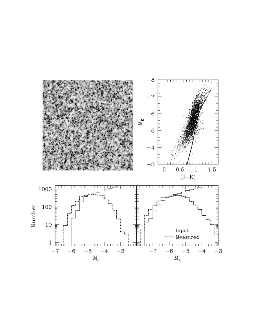
The results of the simulations of a single camera (NIC2) and a single field (F1) are summarized in Figure 12. This is the most crowded field, and hence the effects of blending are the most severe. The simulated -band image is shown in the upper left, and is nearly indistinguishable from the real observations (Fig. 3). The resulting , CMD is shown in the upper right. The input stars form a narrow locus which blends into a line stretching (on this plot) from and to and . The locus of measured stars is broader and shifted brighter and bluer compared to the input stars. As the simulations show, when the field is this crowded, none of our measurements are very accurate.
The input and recovered luminosity functions are shown at the bottom of Figure 12. The -band LFs on the left show that the measured LF is shifted by magnitudes brighter than the input LF. The LFs on the right show that, the -band measurements are not as severely distorted as the undersampled NIC2 -band observations.
7.1 Simulation Results
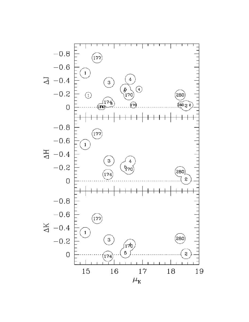
The first statistic we calculate is the difference between the brightest star measured and the brightest star input into each artificial field. This gives a rough idea of the maximum amount of brightening one can expect in each field. Figure 13 illustrates this difference for the ,, and -bands as a function of field surface brightness. This plot shows that there is little brightening due to blending in the artificial fields with lower surface brightnesses (). However, as the surface brightness increases, the amount of artificial brightening increases as well.
The size of each circle in Figure 13 indicates whether the simulation is a NIC1 (small circles) or NIC2 (large circles) field. The higher resolution and more finely sampled NIC1 observations are clearly less affected by blending, with only a few fields having deviations greater than 0.1 magnitudes.
This figure also shows that the brightest -band data are less affected by blending than the corresponding -band measurements. For the most crowded fields (e.g. F1, F177, F174, F3) the -band brightening due to blending can be as high as 0.75 magnitudes, while in the -band, blending is magnitudes less. This can also be seen in the larger difference between the input and recovered LFs at compared to , and the blueward shift of stars in the CMD as seen in Figure 12. As mentioned above, we attribute the difference between & to the undersampling in and the bluer color of the underlying population.
The delta-magnitude quantity previously calculated is admittedly subject to small number statistics, since it is based on only a single star in each field. Ideally we would run each simulation a number of times, and the average difference would be a much more robust estimator of the amount of brightening to expect in the real field. However, looking at the results of all the fields together, the direction and magnitude of the effect is clear.
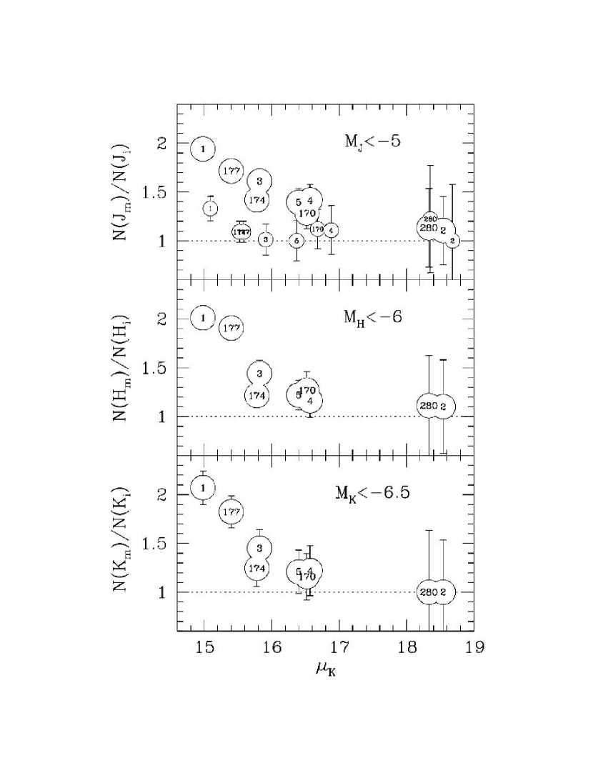
Another interesting, and hopefully more robust, quantity to calculate for each field is the ratio of the number of “bright” stars measured compared to the number of stars input to the same brightness. This quantity is very important, for example when using AGB stars to assess recent star formation. We plot this ratio as a function of the field surface brightness in Figure 14. We chose , , and as the criterion for a star to be considered “bright”. These limits are fairly arbitrary, however if chosen to be much brighter, then some of the fields will have no stars input that bright, and if much fainter, some fields will not be complete to that level, and we will be measuring completeness instead of blending.
Figure 14 shows the ratio of measured to input bright stars for all of our simulated frames. The large circles represent NIC2 fields and the small circles NIC1 fields. The lowest surface brightness fields (F2 & F280) have nearly equal numbers of measured and input stars, i.e. minimal blending. However, as the surface brightness increases, the points begin to move up off of the dashed line indicating a ratio of unity. This upturn is a function of wavelength, but in general occurs at mag/arcsec2 for the NIC2 observations, and mag/arcsec2 for the NIC1 observations. In the simulations of the brightest fields we measure about twice as many bright stars in NIC2, and 1.25 times as many in NIC1 compared to the number which were actually input into the simulation.
Of course the ratio of the number of measured to input stars is dependent on exactly where one draws cutoff magnitude. At brighter cutoff magnitudes the ratio goes to infinity when there are no stars input as bright as we measure. Choosing a fainter cutoff both dilutes the number of blends, and causes faint blends to be lost due to incompleteness.
In summary, both Figures 13 and 14 show similar structure, with a sharp increase in blending between . Obviously the amount of blending one can withstand depends on the scientific goals, however one must be very careful interpreting results from such data. We are even skeptical of some of our own measurements of stars just above the tip of the AGB, which only occur in the most crowded fields where the surface brightness is greater than magnitudes arcsecond-2 (however see §9).
| Recovered | |||
|---|---|---|---|
| Field | Input | Real | Simulation |
| NIC1 | |||
| F1 | 900000 | 4037 | 3277 |
| F2 | 25000 | 348 | 521 |
| F3 | 400000 | 3102 | 3088 |
| F4 | 150000 | 2208 | 2411 |
| F5 | 250000 | 2323 | 2405 |
| F170 | 300000 | 2154 | 2055 |
| F174 | 950000 | 4847 | 4970 |
| F177 | 950000 | 4861 | 4970 |
| F280 | 50000 | 448 | 619 |
| NIC2 | |||
| F1 | 3000000 | 4037 | 3594 |
| F2 | 80000 | 314 | 597 |
| F3 | 1500000 | 3128 | 3498 |
| F4 | 700000 | 2066 | 2598 |
| F5 | 800000 | 2257 | 2555 |
| F170 | 900000 | 1986 | 2496 |
| F174 | 2000000 | 2923 | 3156 |
| F177 | 4000000 | 3221 | 3010 |
| F280 | 110000 | 256 | 487 |
8 Comparison with Previous Observations
8.1 Rich, Mould & Graham (1993)
The groundbased observations of Rich, Mould & Graham (1993, hereafter RMG93) are the foundation of the current work. Theirs was the first study in M31 which systematically attempted to measure the stellar properties over a range of galactocentric distances and bulge-to-disk ratios. For that reason our NIC2 fields were chosen to be the same as those in RMG93. RMG93 took their observations on 1992 Aug 30 – Sept 1 with the Palomar IR imager on the Hale 5m telescope. This instrument was outfitted with a pixel InSb detector with pixels. Each of their fields were observed for 75 seconds through both and filters. Using offsets equal to half the field of view, they obtained 25 frames that were later assembled into mosaics. Thus the central of their mosaics have total integration times of 150s in each filter. The seeing is on these mosaics.
The central of Field 1 from RMG93 is shown on the left side of Figure 15. In order to match up our corresponding NIC2 image shown in the right side of Figure 15, we first rebinned our image by a factor of 4.1 to go from our pixels to the groundbased pixels, then smoothed the rebinned image with a Gaussian kernel to match the seeing in the groundbased images. This rebinned and smoothed intermediary NICMOS image is shown in the center of Fig 15.
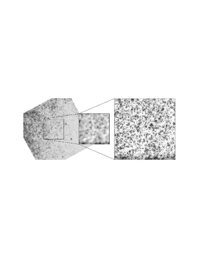
In order to better understand the relationship between the groundbased photometry and our NICMOS measurements we have performed a star-by-star comparison of the objects measured by RMG93 in Field 1. As is obvious from Figure 15, none of the objects seen from the ground correspond to single stars in the NICMOS image. However, if we simply take our brightest measured star nearest the RMG93 object as the center of the clump which composes their object, we can study the composition of that clump.
As an example consider RMG93 star 95. This object is located just above and right of the center of the groundbased image. RMG93 measure this object as , however the star we match this object with has (the first entry in Table 7) . The next star has and lies away. If we include all stars within a radius of we should get approximately the same amount of flux as measured by RMG93 viewed through seeing. Table 7 lists the NICMOS measured stars and their radius from the assumed center of the groundbased clump (columns 2 & 3) and the magnitude of the running sum of their flux (column 4). Going down through this table, we eventually add enough stars to reach the groundbased measurement of at . Of course this radius of equal measurements varies from star to star, depending on how PSFs were fit to the groundbased blends. Using 52 “stars” matched with the RMG93 observations, we find this average radius to be in and in (see Appendix A). Of the 13 stars with matches in field 1, the average difference between the RMG93 measurement and the brightest NICMOS star measured within is magnitudes .
| N | DistanceaaDistance in arcseconds. | Sum | |
|---|---|---|---|
| 1 | 0.01 | 16.63 | 16.63 |
| 2 | 0.15 | 16.35 | 15.73 |
| 3 | 0.25 | 17.87 | 15.59 |
| 4 | 0.25 | 17.24 | 15.37 |
| 5 | 0.44 | 18.68 | 15.32 |
| 6 | 0.47 | 18.49 | 15.26 |
| 7 | 0.48 | 18.75 | 15.22 |
| 8 | 0.51 | 19.47 | 15.20 |
| 9 | 0.52 | 18.84 | 15.16 |
| 10 | 0.52 | 19.27 | 15.14 |
| 11 | 0.57 | 19.47 | 15.12 |
| 12 | 0.59 | 17.09 | 14.96 |
Figure 16 shows a comparison between the NICMOS measured LFs (solid lines) with RMG93’s groundbased LFs (beaded lines). The RMG93 LFs are the measured numbers of stars matched in their and -band images placed into 0.25 magnitude bins (column 2 of their Table 8). We have normalized these LFs by multiplying by 0.063 to compensate for the larger area of the groundbased images (5634 arcsec2) compared to the NIC2 area (355 arcsec2). If the normalized RMG93 LF falls below a value of one (dashed line) it can be taken as the probability that NICMOS would find a star that bright if they exist.
Looking at the comparison in Figure 16 we see that the amount of disagreement is strongly correlated to the field surface brightness, which is listed in the upper left of each panel. Field 1 exhibits the worst case of blending, where RMG93 finds a significant number of stars a magnitude brighter than we measure. Field 3 is not as severe, however the groundbased observations predict that we should find many more bright stars up to mag brighter than we see. The three lowest surface brightness fields (F2, F4, F5) are roughly consistent with the NICMOS measurements. In every field the RMG93 LF trails off to very bright magnitudes, and even though there is a very low probability of finding such bright stars in one of our small NIC2 fields, it seems clear that these are most likely just severe cases of blending.

8.2 Rich & Mould (1991)
Rich & Mould (1991, hereafter RM91) obtained the first infrared color- magnitude diagram of an M31 bulge field, from the nucleus and along the major axis. They observed and -band mosaics of nine non-contiguous fields using the Palomar IR imager on the Hale 5m telescope, yielding a total area of square arcseconds.
The RM91 field lies close to our F3 field, and we compare the luminosity functions by taking the RM91 counts from column 4 (CMD) of their Table 3. We then normalize the RM91 LF by multiplying by the ratio of the NICMOS field F3 area (355 arcsec2) to the RM91 field area. The resulting comparison is shown in Figure 17.
Figure 17 shows remarkable agreement between the bright ends of the NICMOS and RM91 luminosity functions. Had the M31 bulge population been normalized to Baade’s Window in RM91, the apparent extended giant branch would have been far less prominent. However an accurate normalization is difficult without the faint end completeness provided by the NICMOS images.
Figure 17 also shows a discrepancy between the luminosity functions of RM91 and RMG93, where the earlier RM91 groundbased data seems to match the bright end of the NICMOS LF, while the later RMG93 data appears much more affected by blending.
One possible explanation for this difference seems to lie in the analysis of the data. While both datasets were acquired with the same telescope and instrument, the RM91 data were analyzed on a frame-by-frame basis, while the RMG93 data were assembled into a large mosaic before analysis. Therefore the RM91 data retained its original image quality, while the RMG93 image quality, due to difficulties in perfectly registering the frames, was reduced to perhaps even worse than that of the worst image.
In light of our simulations, it is still difficult to understand the apparent agreement between the bright ends of the RM91 and NICMOS luminosity functions. Our simulations (for their quoted seeing) would still lead to the inescapable conclusion that the measured magnitudes of the brightest stars in RM91 must still suffer from crowding. It is also possible that the images may have been so undersampled ( pixels) that that the actual seeing was better than quoted, though RM91 state that 0.6 arcsec seeing was reached in only one of the images. As the original frames are not available, we are not able double check the measurements or to explore the issue in further detail.

8.3 Davidge (2001)
Davidge (2001) has recently obtained images of a bulge field SW of the nucleus of M31 using the 3.6 meter Canada-France-Hawaii Telescope (CFHT). With the help of adaptive optics, his images achieve a FWHM of . His photometric uncertainties include 0.05 magnitudes in the aperture correction and 0.03 magnitudes in the zero-point. The surface brightness of his field (00h42m45.1s, +41°, J2000) is mag/arcsec2 based on the measurements of Kent (1989) and assuming .
Figure 18 shows a comparison between the LFs of the Davidge (2001) field and the two NICMOS fields with bracketing surface brightnesses: F174 and F177, which have and mag/arcsec2 respectively. The Davidge LF should lie between the two NICMOS LFs, however the Davidge LF is instead shifted magnitudes brighter.
Davidge has suggested that the difference between his measurements and our HST-NICMOS observations (Stephens et al., 2001b) is due primarily to calibration. In support of this conclusion he cites simulations which indicate that the effects of blending on his observations are at most 0.1 mag over what would be measured with the NIC2 resolution. However, these simulations used simple Gaussian PSFs and included only stars ( stars/arcsec2). They show only a few severely blended stars which he claims are “easily identifiable”. In reality blending is a stochastic phenomenon, involving millions of stars, and producing a continuum of blending which can be very difficult to detect and quantify.
As shown by Figure 11, making observations at mag/arcsec2 at Davidge’s resolution will give, on average, NRGBT stars per resolution element. Thus in any given resolution element there is a probability of having 2 NRGBT stars, compared to the probability with NICMOS. Thus the most likely cause for the difference between the Davidge (2001) LF and our NICMOS LFs in Figure 18 is indeed due to blending.
As we discussed in Section 7, we are certainly not claiming the comparison of our observations with Davidge (2001) is a case of right and wrong; but rather a case of wrong and wrong. Both sets of observations are affected by blending, and the stars just above the AGB tip in our most crowded fields may in fact be artificially brightened by several tenths of a magnitude.

9 Bright Stars
We have cautioned that some of the bright stars in our fields may be blends of fainter stars, however there exists a population of bright stars which are real. Inspection of the images shows that these stars are obvious point sources, and occur over the entire range of M31 stellar densities. These stars are some of the brightest and bluest which we have observed, with and , and are most likely foreground Milky Way stars. Here we provide a brief discussion of their properties to ensure that they are not confused with a population of young M31 bulge stars.
The CMD of brightest stars measured in all of the NIC2 frames is shown in Figure 19. Here the AGB is located between and extends up to the curved line at . Stars directly above the AGB are most likely blends of fainter stars. However the bright stars bluer than are indeed real stars. If they were at the distance of M31 they would all have bolometric magnitudes brighter than .

We find a total of 8 foreground stars in the NIC2 fields: 2 in F2, 1 in F3, 2 in F4, 1 in F5, 1 in F170, and 1 in the G1 field, which has not been otherwise analyzed in this paper because of the lack of non-cluster stars. We find none in the NIC2 F1, F174, F177, or F280 fields.
Searching the NIC1 observations, we use the fact that the faintest foreground star in the NIC2 group has . Thus if we assume that any star with a NIC1 -band magnitude brighter than is also a MW contaminant, we find 2 in the NIC1 F170 field, and 1 in the F177 field. None of the other 8 NIC1 fields (including G1) have any stars this bright. These three stars are also clearly separated from the rest of the NIC1 AGB LF by a magnitude gap.
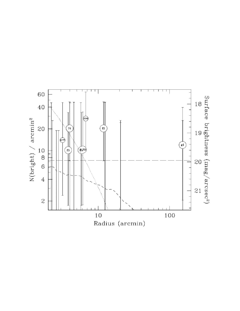
The radial distribution of the bright foreground stars is illustrated in Figure 20. Here we plot the surface density measured in each field as a function of radial distance from the center of M31. The upper and lower limits are one-sigma confidence intervals, calculated using the small-number approximation formulae of Gehrels (1986). The distribution shows no trend with radius, and is certainly not correlated with either of the steeply dropping surface brightness profiles of M31’s bulge or disk, illustrated by the dotted and short-dashed lines respectively.
In total, we find 8 bright foreground stars in the 10 NIC2 fields. These fields have a combined area of 0.95 arcmin2, giving a surface density of 8.4 arcmin2. Although we don’t have color information in the NIC1 frames, there are three very bright stars with . The total area of the NIC1 fields is 0.56 arcmin2, giving a surface density of 5.4 stars arcmin-2 for these bright stars. If we assume that all 11 stars are of the same population, the average surface density is 7.3 stars arcmin-2, which is shown by a long-dashed line in Figure 20.
A comparison with the estimated number of field stars by Ratnatunga & Bahcall (1985) reveals that our measurement of 7.3 stars arcmin-2 is extremely high. The measured mean color of corresponds to for either dwarfs or giants, which means that these stars most likely have . However, Ratnatunga & Bahcall (1985) predict field stars / arcmin2 between and toward M31. Given the combined area of our NIC1 and NIC2 images (1.5 arcmin2), we should have found approximately one field star, not 11.
Unfortunately there have been few surveys of bright field stars toward M31 to verify the model predictions. Ferguson et al. (2002) recently performed a large scale survey of M31 looking for substructure in the halo and disk of M31. Integrating over all their magnitudes, i, which correspond to roughly , they estimate 13,000 - 20,000 Galactic foreground stars deg-2 or between 3.6 - 5.56 stars arcmin-2. This is very close to the prediction of Ratnatunga & Bahcall (1985) for their magnitude range ( /arcmin2), but the stars we have observed mostly have , and thus are too bright to be included in their survey.
Thus while the crowded fields have many blends at , it is clear that the brightest and bluest stars, with and , are real. We find 11 of these stars which is over a factor of 10 greater than what is predicted by Galactic models. However it seems very unlikely that these stars are associated with M31 as their surface density does not scale with the surface brightness of M31, and we find one as far out as the globular cluster G1, 34 kpc from the center of M31.
10 Discussion & Conclusions
We have analyzed the stellar populations of M31 using 9 sets of adjacent HST NIC1 and NIC2 fields, with distances ranging from to from the nucleus. These observations are the highest resolution IR measurements to date, and provide some of the tightest constraints on the maximum luminosities of stars in the bulge of M31.
Analytic estimates of the effects of blending on our observations, where we calculate the number of RGB stars within 1 magnitude of the RGB tip as a function of position in M31, indicate that simulations are required to accurately interpret our observations. We thus perform extensive simulations of each of our NICMOS fields following the procedures of Stephens et al. (2001a). These simulations show that for the most crowded fields we can expect the brightening due to blending to be as high as 0.75 magnitudes in and 0.55 magnitudes in . They also show that the ratio of measured to input bright stars is a strong function of the field surface brightness. In the highest surface brightness field we measure about 25% more bright stars than were input with NIC1, and about twice as many with NIC2.
All of the bulge luminosity functions are consistent with a single, uniform bulge population. This is based on the observation that the small differences we see are correlated with surface brightness, and that the simulations predict similar differences. We note however, that our simulations only verify that a single LF combined with blending can produce the observed field-to-field differences. Thus our observations are consistent with a single bulge LF, but without higher resolution data, small field to field differences cannot be ruled out.
The tip of the RGB in M31 is clearly visible at , and the tip of the bulge AGB extends to . This AGB peak luminosity is significantly fainter than previously claimed. A comparison with the measurements of Rich, Mould & Graham (1993), which guided our choice of the 5 pointed observations, indicates that their brightest stars are most likely severe cases of blending. In a comparison of our F174 and F177 LFs with the recently observed bulge field of Davidge (2001), we find that the magnitude difference between his and our LFs is due entirely to blending in his lower resolution observations, rather than a calibration error as claimed by Davidge.
We also find an unusually high number of bright blueish stars in our fields. In all 20 (NIC1 + NIC2) fields we find 11 stars which are uncorrelated with the surface brightness distribution of M31, and appear to be foreground Milky Way stars. However, the implied surface density of 7.3 arcmin-2 is over a factor of 10 higher than is predicted by Galactic models.
Appendix A NIC1 Transformation
In order to compare observations made with the two different NICMOS cameras with each other and with groundbased observations we must first convert all measurements to a common photometric system. The transformation of NIC2 to the groundbased CIT/CTIO system has already been calculated and published (Stephens et al., 2000). However, NIC1 lacks a formal transformation to any groundbased system.
As a first attempt to transform NIC1 to a groundbased photometric system, we applied the NIC2 transformation from Stephens et al. (2000). Using their calibration keywords, and assuming for the color term, we applied the corresponding offset to all of our NIC1 photometry. However, this transformation yielded large discrepancies (up to magnitudes) between the luminosity functions measured in corresponding NIC1 and NIC2 field pairs, such that the NIC1 fields appeared too faint. A comparison between the STScI calibrated NIC1 and NIC2 F110W luminosity functions shows that the lower surface brightness fields should show nearly perfect agreement, while the more crowded fields should show discrepancies of no more than magnitudes.
As an alternative method to transform NIC1 to a groundbased system, we considered the observations of Rich, Mould & Graham (1993). Our NIC2 observations were chosen to be centered on the RMG93 fields, and since the NIC1 and NIC2 focal planes are so close together ( between field edges) and NICMOS was rotated degrees from North when we took most of our images, NIC1 falls on the lower left (SE) corner of the RMG93 images (see Figure 2). By rebinning and smoothing our NIC1 images we were able to match up 8 “stars” with RMG93. Of course these aren’t really single stars, but rather clumps of many stars. However, by estimating how many stars are in the clumps measured by RMG93, we were able to use their observations to transform ours to the CIT/CTIO system.
Going back to our NIC2 observations, whose calibration we trust, we matched up 52 “stars” with RMG93. Using the -band observations, we determined that we can make NICMOS agree ( magnitudes) with RMG93’s measurements if we sum up all the NICMOS measured stars within a radius around what we estimate to be the center of the RMG93’s “stars”.
To determine the NIC1 transformation, we first calibrate our photometry using the most recent header keywords listed in the NICMOS Data Handbook v5.0 (Dickinson et al., 2002) namely: photfnu = 2.358E-6 Jy sec / DN, and fnuvega = 1773.7 Jy. We then sum the flux of all NICMOS stars measured within of the RMG93 centroids. The resulting difference between the NIC1 magnitudes and RMG93 is magnitudes using all 8 “stars”, or magnitudes using a sigma-rejected sample of 7.
In summary, we apply a magnitude offset to our NIC1 F110W magnitudes to approximately transform them to the -band of the groundbased CIT/CTIO system. This is in contrast to the NIC2 photometry which was transformed using the equations of Stephens et al. (2000), which includes a color term in each band.
References
- Blanco, McCarthy & Blanco (1984) Blanco, V.M., McCarthy, M.F., & Blanco, B.M., 1984, AJ, 89, 636
- Blanco (1986) Blanco, V.M., 1986, AJ, 91, 290
- Davidge (2001) Davidge, T.J., 2001, AJ, 122, 1386
- Davies, Frogel & Terndrup (1991) Davies, R.L., Frogel, J.A., & Terndrup, D.M., 1991, AJ, 102, 1729
- DePoy et al. (1993) DePoy, D.L., Terndrup, D.M., Frogel, J.A., Atwood, B., & Blum, R., 1993, AJ, 105, 2121
- Dickinson et al. (2002) Dickinson, M. E. et al. 2002, in HST NICMOS Data Handbook v. 5.0, ed. B. Mobasher, Baltimore, STScI
- Feltzing & Gilmore (2000) Feltzing, S., & Gilmore, G., 2000, A&A, 355, 949
- Ferguson et al. (2002) Ferguson, A.M., Irwin, M.J., Ibata, R.A., Lewis, G.F., & Tanvir, N.R., 2002, AJ, 124, 1452
- Frogel & Elias (1988) Frogel, J.A., & Elias, J.H. 1988, ApJ, 324, 823
- Frogel & Whitelock (1998) Frogel, J.A., & Whitelock, P.A., 1998, AJ, 116, 754
- Frogel & Whitford (1987) Frogel, J.A., & Whitford, A.E., 1987, ApJ, 320, 199
- Gehrels (1986) Gehrels, N., 1986, ApJ, 303, 336
- Guarnieri, Renzini & Ortolani (1997) Guarnieri, M.D., Renzini, A., & Ortolani, S. 1997, ApJ, 477, L21
- Iben & Renzini (1983) Iben, I. Jr., & Renzini, A., 1983, ARA&A, 21, 271
- Jablonka et al. (1999) Jablonka, P., Bridges, T.J., Sarajedini, A., Meylan, G., Maeder, A., & Meynet, G., 1999, ApJ, 518, 627
- Kent (1989) Kent, S.M., 1989, AJ, 97, 1614
- Kuijken & Rich (2002) Kuijken, K., & Rich, R.M., 2002, AJ, 124, 2054
- MacKenty et al. (1997) MacKenty J.W., et al., 1997, NICMOS Instrument Handbook, Version 2.0, STScI, Baltimore, MD
- McWilliam & Rich (1994) McWilliam, A., & Rich, R.M., 1994, ApJS, 91, 749
- Mould (1986) Mould, J.R., 1986, in Stellar Populations, ed. C. Norman, A. Renzini & M. Tosi, Cambridge University Press, p. 9.
- Ortolani et al. (1995) Ortolani, S., Renzini, A., Gilmozzi, R., Marconi, G., Barbuy, B., Bica, E., & Rich, R. M., 1995, Nature, 377, 701
- Ratnatunga & Bahcall (1985) Ratnatunga, K.U., & Bahcall, J.N., 1985, ApJS, 59, 63
- Renzini (1993) Renzini, A., 1993, in IAU Symp. 153, Galactic Bulges, ed. H. Dejonge & H.J. Habing (Dordrecht: Kluwer), p. 151
- Renzini (1998) Renzini, A., 1998, AJ, 115, 2459
- Rich, Mould & Graham (1993) Rich, R.M., Mould, J.R., & Graham, J.R., 1993, AJ, 106, 2252 (RMG93)
- Rich & Mighell (1995) Rich, R.M., & Mighell, K.J., 1995, ApJ, 439, 145
- Rich et al. (1989) Rich, R.M., Mould, J., Picard, A., Frogel, J.A., & Davies, R., 1989, ApJ, 341, L51
- Rich & Mould (1991) Rich, R.M., & Mould, J., 1991, AJ, 101, 1286
- Stephens et al. (2001a) Stephens, A.W., Frogel, J.A., Freedman, W., Gallart, C., Jablonka, P., Ortolani, S., Renzini, A., Rich, R.M., & Davies, R., 2001a, AJ, 121, 2584
- Stephens et al. (2001b) Stephens, A.W., Frogel, J.A., Freedman, W., Gallart, C., Jablonka, P., Ortolani, S., Renzini, A., Rich, R.M., & Davies, R., 2001b, AJ, 121, 2597
- Stephens et al. (2000) Stephens, A.W., Frogel, J.A., Ortolani, S., Davies, R., Jablonka, P., Renzini, A., & Rich, R.M., 2000 AJ, 119, 419
- Stetson (1990) Stetson, P.B., 1990, PASP, 102, 932
- Stetson (1994) Stetson, P.B., 1994, PASP, 106, 250
- Zoccali et al. (2002) Zoccali, M., Renzini, A., Ortolani, S., Greggio, L., Saviane, I., Cassisi, S., Rejkuba, M., Barbuy, B., Rich, R.M., & Bica, E., 2002, A&A, in press