Reconstruction of the primordial Universe by a Monge–Ampère–Kantorovich optimisation scheme

Abstract

A method for the reconstruction of the primordial density fluctuation field is presented. Various previous approaches to this problem rendered non-unique solutions. Here, it is demonstrated that the initial positions of dark matter fluid elements, under the hypothesis that their displacement is the gradient of a convex potential, can be reconstructed uniquely. In our approach, the cosmological reconstruction problem is reformulated as an assignment problem in optimisation theory. When tested against numerical simulations, our scheme yields excellent reconstruction on scales larger than a few megaparsecs.

I Introduction

The present distribution of galaxies brought to us by redshift surveys indicates that the Universe on large scales exhibits a high degree of clumpiness with coherent structures such as voids, great walls, filaments and clusters. The cosmic microwave background (CMB) explorers, however, indicate that the Universe was highly homogeneous billions of years ago. When studying these data, among the questions that are of concern in cosmology are the initial conditions of the Universe and the dynamics under which it grew into its present form. CMB explorers provide us with valuable knowledge into the initial conditions of the Universe, but the present distribution of the galaxies opens a second, complementary window into its early state.

Unraveling the properties of the early Universe from the present data is an instance of the general class of inverse problems in physics. In cosmology this problem is frequently tackled in an empirical way by taking a forward approach. In this approach, a cosmological model is proposed for the initial power spectrum of dark matter. Next, a particle presentation of the initial density field is made which provides the initial data for an N-body simulation which is run using Newtonian dynamics and is stopped at the present time. Subsequently, a statistical comparison between the outcome of the simulation and the observational data can be made, assuming that a suitable bias relation exists between the distribution of galaxies and that of dark matter. If the statistical test is satisfactory then the implication is that the initial condition was viable; otherwise one changes the cosmological parameters and goes through the whole process again. This is repeated until one obtains a satisfactory statistical test, affirming a good choice for the initial condition.

However, this inverse problem does not have to be necessarily dealt with in a forward manner. Can one fit the present distribution of the galaxies exactly rather than statistically and run it back in time to make the reconstruction of the primordial density fluctuation field? Since Newtonian gravity is time-reversible, one would have been able to integrate the equations of motions back in time and solve the reconstruction problem trivially, if in addition to their positions, the present velocities of the galaxies were also known. As a matter of fact, however, the peculiar velocities of only a few thousands of galaxies are known out of the hundreds of thousands whose redshifts have been measured. Indeed, one goal of reconstruction is to evaluate the peculiar velocities of the galaxies and in this manner put direct constraints on cosmological parameters.

Without a second boundary condition, reconstruction would thus be an infeasible task. Newton’s equation of motion requires two boundary conditions, whereas, for reconstruction so far we only have mentioned the present positions of the galaxies. The second condition is the homogeneity of the initial density field: as we go back in time the peculiar velocities of the galaxies vanish. Thus, contrary to the forward approach where one solves an initial-value problem, in the reconstruction approach one is dealing with a two-point boundary value problem. In the former, one starts with the initial positions and velocities of the particles and solves Newton’s equations arriving at a unique final position and velocity for a given particle. In the latter one does not always have uniqueness. This has been one of the shortcomings of reconstruction, which was consequently taken to be an ill-posed problem.

In this work, we report on a new method of reconstruction which guarantees uniqueness (Frisch et al. 2002). In Section II, we review the previous works on reconstruction. We describe our mathematical formulation of the reconstruction problem in Section III and show that the cosmological reconstruction problem, under our hypotheses, is an example of assignment problems in optimisation theory. In Section IV, we describe the numerical algorithms to solve the assignment problem. In Section V, we test our reconstruction method with numerical N-body simulation both in real and redshift spaces. Section VI contains our conclusions.

II A brief review of Variational and Eulerian and Lagrangian approaches to reconstruction

The history of reconstruction goes back to the work of Peebles (Peebles 1989) on tracing the orbits of the members of the local group. In his approach, reconstruction was solved as a variational problem. Instead of solving the equations of motion, one searches for the stationary points of the corresponding Euler-Lagrange action. The action in the comoving coordinates is (Peebles 1980)

$$S=\int_{0}^{t_{0}}dt\,\left[{m_{i}a^{2}\dot{\bf x}_{i}^{2}\over 2}-{Gm_{i}m_{j}\over a|{\bf x}_{i}-{\bf x}_{j}|}+{2\over 3}\pi G\rho_{\rm b}a^{2}m_{i}{\bf x}_{i}^{2}\right]\;,$$ (1)

where summation over repeated indices and $j\not=i$ is implied, $t_{0}$ denotes the present time, the path of the $i$th particle with mass $m_{i}$ is ${\bf x}_{i}(t)$, $\rho_{\rm b}$ is the mean mass density, and the present value of the expansion parameter $a(t)$ is $a_{0}=a(t_{0})=1$. The equation of motion is obtained by requiring

$$\delta S=\int_{0}^{t_{0}}dt\left[{\partial{\cal L}\over\partial{\bf x}_{i}}\cdot\delta{\bf x}_{i}+{\partial{\cal L}\over\partial\dot{\bf x}_{i}}\cdot{\delta\dot{\bf x}_{i}}\right]=0\;,$$ (2)

which leads to

$$\int_{0}^{t_{0}}dt\delta{\bf x}_{i}\left[\sum_{j\not=i}{Gm_{i}m_{j}({\bf x}_{i}-{\bf x}_{j})\over a|{\bf x}_{i}-{\bf x}_{j}|^{3}}+{4\over 3}\pi G\rho_{\rm b}a^{2}m_{i}{\bf x}_{i}-m_{i}{\partial\over\partial t}(a^{2}\dot{\bf x}_{i}^{2})\right]-m_{i}\left[a^{2}\dot{\bf x}_{i}\cdot\delta{\bf x}_{i}\right]^{t_{0}}_{0}=0\;.$$ (3)

The boundary conditions

$$\delta{\bf x}_{i} = 0\qquad{\rm at}\qquad t=t_{0}$$ (4)

$$a^{2}\dot{\bf x}_{i} = 0\qquad{\rm as}\qquad t\rightarrow 0$$ (5)

would then eliminate the boundary terms in (3).

The components $\alpha=1,2,3$ of the orbit of the $i$th particle are modeled as

$$x_{i}^{\alpha}=x_{i}^{\alpha}(t_{0})+\sum_{n}C_{i,n}^{\alpha}f_{n}(t)\;.$$ (6)

The functions $f_{n}$ are normally convenient functions of the scale factor $a$ and should satisfy the boundary conditions (5). Initially, trial functions such as $f_{n}=a^{n}(1-a)$ or $f_{n}={\rm sin}\left({n\pi a/2}\right)$ with $f_{0}={\rm cos}\left({\pi a/2}\right)$ were used. The coefficients $C_{i,n}$ are then found by substituting expression (6) in the action (1) and finding the stationary points. That is for physical trajectories

$${\partial S\over\partial C_{i,n}}=0\;,$$ (7)

leading to

$$m_{i}\int_{0}^{t_{0}}dtf_{n}(t)\left[-{d\over dt}a^{2}{dx_{i}^{\alpha}\over dt}+{4\over 3}\pi G\rho_{\rm b}a^{2}x_{i}^{\alpha}(t)\right]=-{G\over a}\int^{t_{0}}_{0}dt\sum_{j}m_{j}{x_{j}^{\alpha}-x_{i}^{\alpha}\over|{\bf x}_{i}-{\bf x}_{j}|}\;.$$ (8)

In his first work, Peebles (1989) considered only the minimum of the action, while reconstructing the trajectories of the galaxies back in time. In a low-density Universe, assuming a linear bias, the predicted velocities agreed with the observed ones for most galaxies of the local group but failed with a large discrepancy for the remaining members. Later on, it was found that when the trajectories corresponding to the saddle-point of the action were taken instead of the minimum, much better an agreement between predicted and observed velocities was obtained, for almost all the galaxies in the local group (see Fig. 1). Thus, by adjusting the orbits until the predicted and observed velocities agreed, reasonable bounds on cosmological parameters were found (Peebles 1989, 1990).

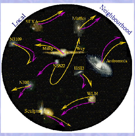
FIG. 1.: A schematic demonstration of Peebles’ reconstruction of the trajectories of the members of the local neighbourhood using a variational approach based on the minimisation of Euler–Lagrange action. The arrows go back in time, starting from the present and pointing towards the initial positions of the sources. In most cases there is more than one allowed trajectory due to orbit crossing (closely related to the multistreaming of the underlying dark matter fluid). The pink (darker) orbits correspond to taking the minimum of the action whereas the yellow (brighter) orbits were obtained by taking the saddle-point solution. Of particular interest is the orbit of N6822 which in the former solution is on its first approach towards us and in the second solution is in its passing orbit. A better agreement between the evaluated and observed velocities was shown to correspond to the saddle point solution.

Although rather successful when applied to catalogues such as NGB (Tully 1988), reconstruction with such an aim, namely establishing bounds on cosmological parameters using measured peculiar velocities, could not be applied to larger galaxy redshift surveys, containing hundreds of thousands of galaxies for the majority of which the peculiar velocities are unknown. For large datasets, it is not possible to use the velocities, to choose the right orbit from the many which are all physically possible. In order to resolve the problem of multiple solutions (the existence of many mathematically possible orbits) one normally had to do significant smoothing and then try the computationally costly reconstruction using Peebles variational approach (Shaya et al. 1995, Branchini et al. 2001). However, one was still not guaranteed to have chosen the right orbit (see Hjorteland 1999 for a review of the action variational method).

The multiple solution can be caused by various factors. For example, the discretisation in the numerical integrations (8) can produce spurious valleys in the landscape of the Euler–Lagrange action. However, even overcoming all these numerical artifacts one is still not guaranteed uniqueness. There is a genuine physical reason for the lack of uniqueness which is often referred to in cosmology as multistreaming. Cold dark matter (CDM) is a collisionless fluid with no velocity dispersion. An important feature that arises in the course of the evolution of a self-gravitating CDM Universe is the formation of multistream regions on which the velocity field is non-unique. These regions are bounded by caustics at which the density is divergent. At a multistream point where velocity is multiple-valued, a particle can have many different mathematically viable trajectories each of which would correspond to a different stationary point of the Euler–Lagrange action which is no-longer convex.

In addition to the variational approach to reconstruction, there is the well-known POTENT reconstruction of the three-dimensional velocity field from its radial component (Dekel et al. 1990). The POTENT method is the non-iterative Eulerian version of the original iterative Lagrangian method (Bertschinger and Dekel 1989) and assumes potential flow in Eulerian space. POTENT finds the velocity potential field by integrating the radial components of the velocities along the line of sight. Since this is an Eulerian method, its validity does not extend much beyond the linear Eulerian regime.

In following works, with the use of POTENT-reconstructed velocity field or the density field obtained from the analysis of the redshift surveys, the gravitational potential field was also reconstructed (Nusser and Dekel 1992). The gravitational potential was then traced back in time using the so-called Zel’dovich–Bernoulli equation which combines the Zel’dovich approximation with the Euler momentum conservation equation. Later on, it was further shown (Gramann 1993) that the initial gravitational potential is more accurately recovered using the Zel’dovich-continuity equation which combines the Zel’dovich approximation with the mass continuity equation (Nusser et al. 1991). The Eulerian formulations of Zel’dovich approximation was also extended to second-order and it was found that this extension does not give significant improvement in the reconstruction (Monaco and Efstathiou 1999, see Sahni and Coles 1995 for various approximation schemes).

However, these procedures are valid only as long as the density fluctuations are in the Eulerian linear or quasi-linear regimes (defined by $|(\rho-\rho_{\rm b})/\rho_{\rm b}|\leq 1$). They do not robustly recover the initial density in regions of high density when the present-day structures are highly nonlinear ($|(\rho-\rho_{\rm b})/\rho_{\rm b}|\gg 1$). Therefore, they require that the final density field be smoothed quite heavily to remove any severe nonlinearities, before the dynamical evolution equations are integrated backward in time.

Here, we describe a new method of reconstruction (Frisch et al. 2002) which not only overcomes the problem of nonuniqueness encountered in the least-action-based methods but also remains valid well beyond the linear Eulerian approximations employed in many other popular reconstruction methods, a few of which have been mentioned previously.

III Monge–Ampère–Kantorovich reconstruction

Thus, reconstruction is a well-posed problem for as long as we avoid multistream regions. The mathematical formulation of this problem is as follows (Frisch et al. 2002). Unlike most of the previous works on reconstruction where one studies the Euler-Lagrange action, we start from a constraint equation, namely the mass conservation,

$$\rho({\bf x})d{\bf x}=\rho_{0}({\bf q})d{\bf q}\;,\qquad$$ (9)

where $\rho_{0}({\bf q})$ is the density at the initial (or Lagrangian) position, ${\bf q}$, and $\rho({\bf x})$ is the density at the present (or Eulerian) position, ${\bf x}$, of the fluid element. The above mass conservation equation can be rearranged in the following form

$${\rm det}\left[{\partial q_{i}\over\partial x_{j}}\right]={\rho({\bf x})\over\rho_{0}({\bf q})}\;,$$ (10)

where ${\rm det}$ stands for determinant and $\rho_{0}({\bf q})$ is constant. The right-hand-side of the above expression is basically given by our boundary conditions: the final positions of the particles are known and the initial distribution is homogeneous, $\rho_{0}({\bf q})={\rm const}$. To solve the equation, we make the following two hypotheses: first that the Lagrangian map (${\bf q}\rightarrow{\bf x}$) is the gradient of a potential $\Phi$ and second that the potential $\Phi$ is convex . That is

$${\bf x}({\bf q},t)=\nabla_{q}\Phi({\bf q},t)\;.$$ (11)

The convexity guarantees that a single Lagrangian position corresponds to a single Eulerian position, i.e., there has been no multistreaming . These assumptions imply that the inverse map ${\bf x}\rightarrow{\bf q}$ has also a potential representation

$${\bf q}={\bf\nabla}_{\bf x}\Theta({\bf x},t)\;,$$ (12)

where the potential $\Theta({\bf x})$ is also a convex function and is related to $\Phi({\bf x})$ by the Legendre–Fenchel transform (e.g. Arnold 1978)

$$\Theta({\bf x})=\max_{\bf q}\left[{\bf q}\cdot{\bf x}-\Phi({\bf q})\right]\qquad;\qquad\Phi({\bf q})=\max_{\bf x}\left[{\bf x}\cdot{\bf q}-\Theta({\bf x})\right]\;.$$ (13)

The inverse map is now substituted in (10) yielding

$${\rm det}\left[{\partial^{2}\Theta({\bf x},t)\over\partial x_{i}\partial x_{j}}\right]={\rho({\bf x})\over\rho_{0}({\bf q})}\;,$$ (14)

which is the well-known Monge–Ampère equation. The solution to this 222 years old problem has recently been discovered (Brenier 1987, Benamou and Brenier 2000) when it was realised that the map generated by the solution to the Monge–Ampère equation is the unique solution to an optimisation problem. This is the Monge–Kantorovich mass transportation problem, in which one seeks the map ${\bf x}\rightarrow{\bf q}$ which minimises the quadratic cost function

$$I=\int_{\bf q}\rho_{0}({\bf q})|{\bf x}-{\bf q}|^{2}d^{3}q=\int_{\bf x}\rho({\bf x})|{\bf x}-{\bf q}|^{2}d^{3}x\;.$$ (15)

A sketch of the proof is as follows. A small variation in the cost function yields

$$\delta I=\int_{\bf x}\left[2\rho({\bf x})({\bf x}-{\bf q})\cdot\delta{\bf x}\right]d^{3}x\;,$$ (16)

which must be supplemented by the condition

$${\bf\nabla}_{\bf x}\cdot\left(\rho({\bf x})\delta{\bf x}\right)=0\;,$$ (17)

which expresses the constraint that the Eulerian density remains unchanged. The vanishing of $\delta I$ should then hold for all ${\bf x}-{\bf q}$ which are orthogonal (in $L^{2}$) to functions of zero divergence. These are clearly gradients. Hence ${\bf x}-{\bf q}({\bf x})$ and thus ${\bf q}(\bf x)$ is a gradient of a function of ${\bf x}$.

Discretising the cost (15) into equal mass units yields

$$I=\min_{j(\cdot)}\left(\sum_{i=1}^{N}\left({\bf q}_{j(i)}-{\bf x}_{i}\right)^{2}\right)\;.$$ (18)

The formulation presented in (18) is known as the assignment problem: given $N$ initial and $N$ final entries one has to find the permutation which minimises the quadratic cost function (see Fig. 2).

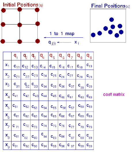
FIG. 2.: Solving the reconstruction problem as an assignment problem. An example of a system of $N=9$ particles is sketched. The cost matrix is shown. For example the entry ${\rm C}_{32}$ is the cost of getting from the Lagrangian position ${\bf q}_{2}$ to the Eulerian position ${\bf x}_{3}$. The cost of this transport is ${\rm C}_{32}=({\bf q}_{2}-{\bf x}_{3})^{2}$. The total cost, ${\rm C_{T}}$ of a given permutation is the sum of all such costs which are chosen for that permutation. That is ${\rm C_{T}}=\sum_{i}{\rm C}_{ij(i)}$. Generally, there are $N!$ possible permutations. Only one of these $N!$ permutations is the optimal assignment: ${\rm C_{optimal}}=\min_{j(i)}({\rm C_{T}})$. For this system there are 362,880 different costs possible, each obtained by a different permutation. Algorithms with factorial complexity are clearly impractical even for small systems. However, assignment algorithms have complexities of polynomial degrees.

IV Solving the assignment problem

If one were to solve the assignment problem for $N$ particles directly, one would need to search among $N!$ possible permutations for the one which has the minimum cost. However, advanced assignment algorithms exist which reduce the complexity of the problem from factorial to polynomial (so far for our problem as verified by numerical tests for $N<20,000$, e.g., Burkard and Derigs 1980 algorithm has a complexity of $N^{3.6}$ for a constant-volume sampling of particles and a complexity of $N^{2.8}$ for a constant-density sampling. The Bertsekas 1998 auction algorithm has a complexity of $N^{2.2}$ in both cases). Before discussing these methods, let us briefly comment on a class of stochastic algorithms, which do not give uniqueness and hence should be avoided.

In the PIZA method of solving the assignment problem (Croft & Gaztañaga 1997), initially a random pairing between $N$ Lagrangian and $N$ Eulerian coordinates is made. Starting from this initial random one-to-one assignment, subsequently a pair (corresponding to two Eulerian and two Lagrangian positions) is chosen at random. For example, let us consider the randomly-selected pair ${\bf x_{1}}$ and ${\bf x_{2}}$ which have been assigned in the initial random assignment to ${\bf q}_{1}$ and ${\bf q}_{2}$ respectively. Next one swaps their Lagrangian coordinates and assigns ${\bf x_{1}}$ to ${\bf q}_{2}$ and ${\bf x_{2}}$ to ${\bf q}_{1}$ in this example. If

$$\left[({\bf x}_{1}-{\bf q}_{1})^{2}+({\bf x}_{2}-{\bf q}_{2})^{2}\right]>\left[({\bf x}_{1}-{\bf q}_{2})^{2}+({\bf x}_{2}-{\bf q}_{1})^{2}\right]\;,$$ (19)

then one swaps the Lagrangian positions, otherwise, one keeps the original assignment. This process is repeated until one is convinced that a lower cost cannot be achieved. However, in this manner there is no guarantee that the optimal assignment has been achieved and the true minimum cost has been found. Moreover, there is a possibility of deadlock when the cost can be decreased only by a simultaneous interchange of three or more particles, while the PIZA algorithm reports a spurious minimum of the cost with respect to two-particle interchanges. Results obtained in this way depend strongly on the choice of initial random assignment and on the random selection of the pairs and suffer severely from the lack of uniqueness (see Fig. 3).

In spite of these problems associated with PIZA-type algorithms in solving the assignment problem, it has been shown (Narayanan and Croft 1999) in a point-by-point comparison of the reconstructed with the true initial density field from a N-body simulation, that PIZA performs better than other methods such as those based on a Eulerian formulation of the Zel’dovich approximation (discussed at the end of Section II).

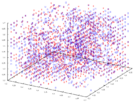
FIG. 3.: The lack of uniqueness in the results of two runs using a stochastic algorithm to solve the assignment problems. In the stochastic algorithm, based on pair-interchange, one searches for, what is frequently referred to in pure mathematics as, a monotonic map instead of a true cyclic monotone map. The red and blue points (stars and boxes respectively) are the perfectly-reconstructed Lagrangian positions using the same stochastic code with two different random seeds. The outputs of the two runs do not coincide, meaning that the reconstructed Lagrangian positions (and hence peculiar velocities) depend on the initial random assignment and on the random pair interchange. The lack of uniqueness in this case is superficial and a shortcoming of the chosen numerical method. Such difficulties do not arise when deterministic algorithms are used to solve the assignment problem.

There are various deterministic algorithms which guarantee that the optimal assignment is found. An example is an algorithm written by Hénon (Hénon 1995), demonstrated in Fig. 4. In this approach, a simple mechanical device is defined and then simulated which solves the assignment problem. The device acts as an analog computer: the numbers entering the problem are represented by physical quantities and the equations are replaced by physical laws.

One starts with $N$ columns $B$s (which represent the Lagrangian positions of the particles) and $N$ rows, $A$s (which represent the Eulerian positions of the particles). On each row there are $N$ studs whose lengths are directly related to the distances between that row and each column. The columns are given negative weights of $-1$ and act as floats and the rows are given weights of $1$.

The potential energy of the system shown in Fig. 4, within an additive constant, is

$$U=\sum_{i}\alpha_{i}-\sum_{j}\beta_{j}\;,$$ (20)

where $\alpha_{i}$ is the height of the row $A_{i}$ and $\beta_{j}$ is the height of the column $B_{j}$, since all rows and columns have the same weight ($1$ and $-1$ respectively).

Initially, all rods are maintained at a fixed position by two additional rods $P$ and $Q$ with the row $A_{i}$ above column $B_{j}$, so that there is no contact between the rows and the studs. Next, the rods are released by removing the holds $P$ and $Q$ and the system starts evolving: rows go down and columns go up and the contacts are made with the studs. Aggregates of rows and columns are progressively formed. As new contacts are made, these aggregates are modified and thus a complicated evolution follows which is graphically demonstrated with a simple example in Fig. 5. One can then show that an equilibrium where the potential energy (20) of the system is minimum will be reached after a finite time. It can then be shown (Hénon 1995) that if the system is in equilibrium and the column $B_{j}$ is in contact with row $A_{i}$ then the force $f_{ij}$ is the optimal solution of the assignment problem. When $f_{ij}$ is equal to one there is an assignment between rows and columns and when $f_{ij}$ is equal to zero there is no assignment. The potential energy of the corresponding equilibrium is equivalent to the total cost of the optimal solution.

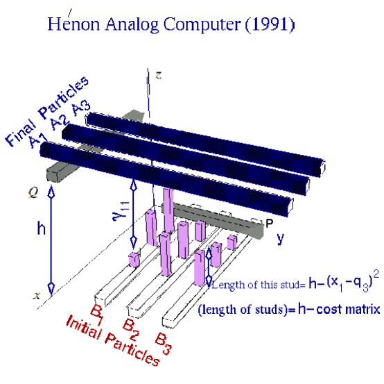
FIG. 4.: Hénon’s mechanical device which solves the assignment problem. The device acts as an analog computer. The rows $A_{i}$ remain parallel to the $y$ axis, are constrained to move vertically and have positive weights. The columns $B_{j}$ remain parallel to the $x$ axis, can only move vertically and have negative weights. Vertical studs are placed on the columns, in such a way that each stud enforces a minimal distance between row $A_{i}$ and column $B_{j}$. Initially all rods are kept at fixed positions by stops $P$ and $Q$. Then the rods are released by removing the stops $Q$ and $P$ and the system starts evolving. Rows go down and columns go up and aggregates of rows and columns are made. Thus a complex evolution takes place. The rules for the formation of aggregates are demonstrated by a simple example in the figure that follows.

.

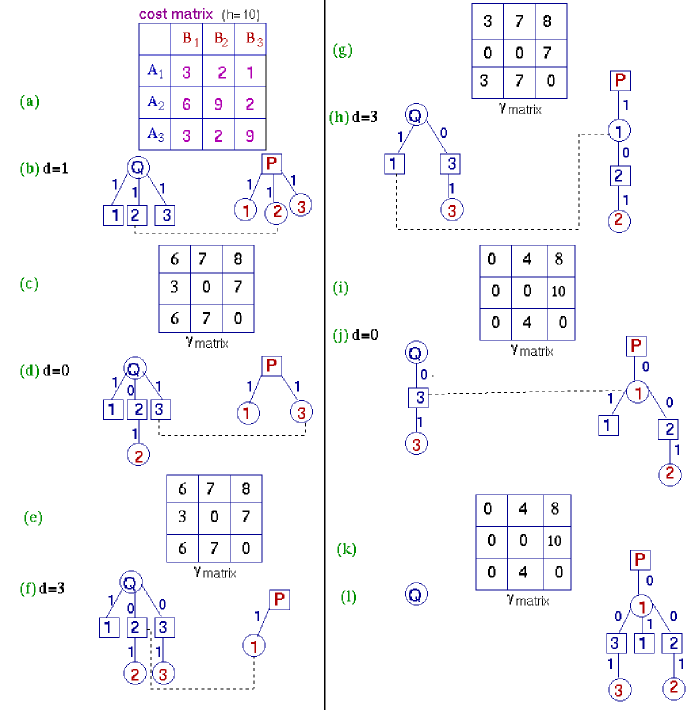
FIG. 5.: A step-by-step (a to l) progress of Hénon’s algorithm on a simple example with three initial and final positions (columns and rows) is shown. The table on the top left shows the values of the costs (distances between rows and columns). When executing the algorithm by hand, it is convenient to keep track of the distances between the rows and the studs, i.e. the quantities $\gamma_{ij}=\alpha_{i}-\beta_{j}-c_{ij}$ where $\alpha_{i}$ is the variable height of the row $A_{i}$ and $\beta_{j}$ is the variable height of the column $B_{j}$. A graph of the initial state is made with the first contact being made between the second row and second column which have the largest cost (note that the code originally written by Hénon, in fact, finds the maximum cost. For our purpose of finding the minimum cost, one can just simply subtract the matrix elements $c_{ij}$ from a large number). Thus, at this point the entries in the $\gamma$ matrix change since now the second row and column are in contact and hence $c_{22}=0$. Obviously the distances between all other rows and columns should also be modified. The second matrix shows the new distances and automatically a contact is made between third row and third column whose separation is now also zero. Since the second and third rows cannot move now, the next contact is made between the first column and the second row and the break occurs where the total force on the branch is weakest. Since this is where the second row meets the support $Q$, part of the $Q$ tree is captured by the $P$ tree, as demonstrated. The next contact can now only be made between the first row and the first column and the break occurs at the weakest branch. The equilibrium position is now reached where each row is supported by one column. In the final optimal assignment column 1 is attached to row 1, column 2 goes to row 2 and column 3 is associated to row 3. For this simple exercise one can easily see that this procedure achieves the maximum cost (which in this example is $21$).

V Test of Monge–Ampère–Kantorovich (MAK) reconstruction with N-body simulations

Thus, in our reconstruction method, the initial positions of the particles are uniquely found by solving the assignment problem. This result was based on our reconstruction hypothesis. We could test the validity of our hypothesis by direct comparison with numerical N-body simulations which is what we shall demonstrate later in this section. However, it is worth commenting briefly on the theoretical, observational and numerical justifications for our hypothesis. It is well-known that the Zel’dovich approximation (Zel’dovich 1970) works well in describing the large-scale structure of the Universe. In the Zel’dovich approximation particles move with their initial velocities on inertial trajectories in appropriately redefined coordinates. It is also known that the irrotationality of the particle displacements (expressed in Lagrangian coordinates) remains valid even at the second-order in the Lagrangian perturbation theory (Moutarde et al. 1991; Buchert 1992; Munshi et al. 1994; Catelan 1995). This provides the theoretical motivation for our first hypothesis. The lack of severe multistream regions is confirmed by the geometrical properties of the cosmological structures. In the presence of significant multistreaming such as the one that occurs in Zel’dovich approximation, one could not expect the formation of long-lived structures such as filaments and walls which is observed in numerical N-body simulations. In the presence of significant multistreaming these structures would form and would smear out and disappear rapidly. This is not backed by numerical simulations. The latter show the formation of shock-like structures well-described by Burgers model (a model of shock formation and evolution in a compressible fluid), which has been extensively used to describe the large-scale structure of the Universe (Gurbatov & Saichev 1984; Gurbatov, Saichev & Shandarin 1989; Shandarin & Zel’dovich 1989; Vergassola et al. 1994). The success of Burgers model indicates that a viscosity-generating mechanism operates at small scales in collisionless systems resulting in the formation of shock-like structures rather than caustic-like structures.

In spite of this evidence in support of our reconstruction hypothesis, one needs to test it before applying it to real galaxy catalogues. We have tested our reconstruction against numerical N-body simulation. We ran a $\Lambda$CDM simulation of $128^{3}$ dark matter particles, using the adaptive P³M code HYDRA (Couchman et al. 1995). Our cosmological parameters are $\Omega_{m}=0.3,\Omega_{\lambda}=0.7,h=0.65,\sigma_{8}=0.9$ and a box size of $200$Mpc/h. We took two sparse samples of $17,178$ and $100,000$ particles corresponding to grids of $6$Mpc and $3$Mpc respectively, at $z=0$ and placed them initially on a uniform grid. For the $17,178$ particle reconstruction, the sparse sampling was done by first selecting a subset of $32^{3}$ particles on a regular Eulerian grid and then selecting all the particles which remained inside a spherical cut of radius half the size of the simulation box. The sparse sample of $100,000$ points was made randomly. An assignment algorithm, similar to that of Hénon described in the previous section, is used to find the correspondence between the Eulerian and the Lagrangian positions. The results of our test are shown in Fig. 6.

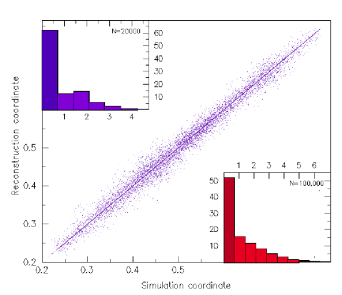
FIG. 6.: Test of MAK reconstruction of the Lagrangian positions, using a $\Lambda$CDM simulation of $128^{3}$ particles in a box of size $200~{}{\rm Mpc}^{3}/h^{3}$. In the scatter plot, the dots near the diagonal are a scatter plot of reconstructed initial points versus simulation initial points for a grid of size $6$ Mpc/h with about 20,000 points. The scatter diagram uses a quasi-periodic projection coordinate ${\tilde{\bf q}}\equiv(q_{x}+\sqrt{2}q_{y}+{\sqrt{3}}q_{z})/(1+\sqrt{2}+\sqrt{3})$ which guarantees a one-to-one correspondence between $\tilde{\bf q}$ values and points on the regular Lagrangian grid. The upper left inset is a histogram (by percentage) of distances in reconstruction mesh units between such points; the first bin corresponds to perfect reconstruction; the lower-inset is a similar histogram for reconstruction on a finer grid of about $3$ Mpc/h using $100,000$ points. With the $6$ Mpc/h grid $62\%$ of the points, and with $3$ Mpc/h grid more than $50\%$ of the points, are assigned perfectly.

It is instructive to compare our results presented in Fig. 6 with those obtained by a stochastic PIZA-type algorithms. Fig. 7 demonstrates such a comparison. We see that not only the stochastic algorithms do not guarantee uniqueness, as demonstrated in Fig. 3, but also the number of exactly reconstructed points by these algorithms are much below those obtained by our deterministic algorithm.

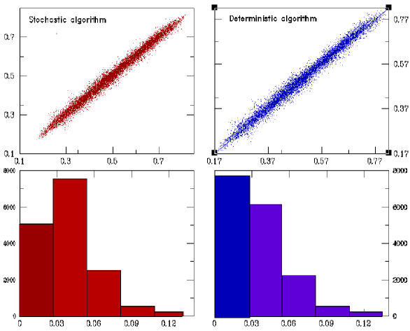
FIG. 7.: A comparison of a PIZA-type, stochastic method, versus our MAK, deterministic method of solving the assignment problem is shown. The outputs of the simulation used for Fig. 6 have also been used here. In the stochastic method, almost one billion pair interchange are made. At which point the cost-reduction cannot be reduced anymore. However, even with such a large number of interchanges, the number of exactly reconstructed points is well below that achieved by MAK. The upper sets are the scatter plots of reconstructed versus simulation Lagrangian positions for PIZA (left top set) and for MAK (right top set). The lower sets are histograms of the distances between the reconstructed Lagrangian positions and those given by the simulation. The bin sizes are taken to be slightly less than one mesh. Hence, all the points in the first (darker) bin correspond to those which have been exactly reconstructed. Using PIZA, we achieve a maximum of about $5000$ out of the $17,178$ points exactly-reconstructed positions whereas with MAK this number reaches almost $8000$ out of $17,178$ points. Note that, for the sole purpose of comparing MAK with PIZA it is not necessary to account for periodicity corrections, which would improve both performances equally. Accounting for the periodicity improves exactly-reconstructed MAK positions to almost $11,000$ points out of $17,178$ points used for reconstruction, as shown in the upper inset of Fig. 6. Starting with an initial random cost of about 200 million (Mpc/h)² ($5000$ in our box unit which runs from zero to one), after one billion pair interchange, a minimum cost of about 1,960,000 (Mpc/h)² ($49$ in our box unit) is achieved. Continuing to run the code on a 2  GHz DEC alpha workstation, consuming almost a week of CPU time, does not reduce the cost any further. With the MAK algorithm, the minimum cost is achieved, on the same machine, in a few minutes. The cost for MAK is 1,836,000 (Mpc/h)² ($45.9$ in box units) which is significantly lower than the minimum cost of PIZA. Considering that the average particle displacement in one Hubble time is about $10$ Mpc/h (about $1/20$ of the box size) this discrepancy between MAK and PIZA costs is rather significant.

When reconstructing from observational data, in redshift space, the galaxies positions are displaced radially by an amount proportional to the radial component of the peculiar velocity in the line of sight. Thus for real catalogues, the cost minimisation need be performed using redshift space coordinates (Valentine et al. 2000). The redshift position of a galaxy is given by

$${\bf s}={\bf x}+\hat{\bf s}\left({\dot{\bf x}\over H}\cdot\hat{\bf s}\right)\;,$$ (21)

where under our assumption of irrotationality and convexity of the Lagrangian map and to first order in Lagrangian perturbation theory,

$$\dot{\bf x}=\beta H({\bf x}-{\bf q})$$ (22)

and $\beta={f(\Omega)/b}$ with $f(\Omega)=d{\rm ln}\delta/d{\rm ln}a=\Omega_{\rm m}^{0.6}$ and the bias factor is $\delta_{\rm galaxies}=b\delta_{\rm mass}$. The quadratic cost function can then be easily found in terms of redshift space coordinates as follows

$$({\bf x}-{\bf q})^{2}=({\bf s}-{\bf q})^{2}-{\beta(2+\beta)\over(1+\beta)^{2}}\left(({\bf s}-{\bf q})\cdot\hat{\bf s}\right)^{2}\;.$$ (23)

Using MAK, based now on the modified cost (18) we can then find the corresponding ${\bf q}$ for each ${\bf s}$ and hence find the peculiar velocities. Indeed, using (21)

$${\bf s}-{\bf q}={\dot{\bf x}\over H}\left(1+{b\over\Omega_{\rm m}^{0.6}}\right)\;.$$ (24)

Note that in this approach the motion of the local group itself is ignored, which however should also be accounted for (Taylor & Valentine 1999). Furthermore, the effect of catalogue selection function can be handled by giving each galaxy an effective-mass inversely proportional to the catalogue selection function (Nusser and Branchini 2000). We have also assumed that galaxies are unbiased tracers of the mass distribution. However, the relative bias between galaxies of different luminosities and of different morphological types indicate that galaxies are likely to be biased tracers of mass distribution (e.g. Loveday et al. 1995). Biasing can be taken into account in a similar manner to the catalogue selection function (Nusser and Branchini 2000). The net effect of biasing for our scheme is that it changes the effective-mass associated to the galaxies which can be easily incorporated in our cost function (18), by multiplying the quadratic function inside the sum by the effective-mass $m_{i}$ associated with each Eulerian position ${\bf x}_{i}$.

We have also performed MAK reconstruction with the redshift-modified cost function which led to somewhat degraded results but at the same time provided an approximate determination of peculiar velocities (see Fig. 8). A more accurate determination of peculiar velocities can be made using second-order Lagrangian perturbation theory (e.g. Catelan 1995 and refs. therein).

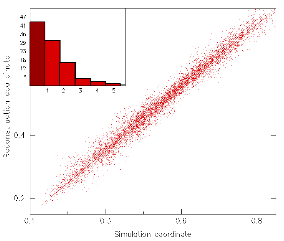
FIG. 8.: Reconstruction test in redshift space with the same data as that used for real-space reconstruction tested in the upper left histogram of Fig. 6. The velocities are smoothed over a sphere of radius $2$ Mpc/h. The observer is taken to be at the centre of the simulation box. The Lagrangian reconstructed points are plotted against the simulation Lagrangian positions using the quasi-periodic projection coordinates used for the scatter plot of Fig. 6. The histogram corresponds to the distances between the reconstructed and the simulation Lagrangian positions for each Eulerian position. The bins of the histogram are smaller than one mesh and the first one corresponds to exactly-reconstructed Lagrangian positions. We obtain $43\%$ perfect reconstruction.

We have also compared the redshift-space MAK reconstruction to real space MAK reconstruction, which shows that almost $50\%$ of exactly-reconstructed positions correspond to the same points (see Fig. 9). This test shows that MAK is robust against systematic errors.

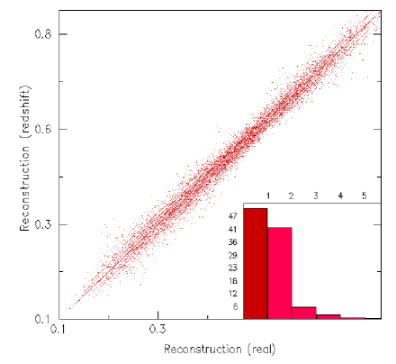
FIG. 9.: Comparison of redshift versus real space reconstruction allows a test of the robustness of MAK reconstruction against systematic errors. The same data as those used for Fig. 8 has been used to obtain the above result. In both real and redshift space most of the exactly reconstructed points almost $50\%$ of the points, which fall in the first bin of the histogram, correspond to the same particles.

Therefore the question that one asks at this point is: where does reconstruction perform poorly?

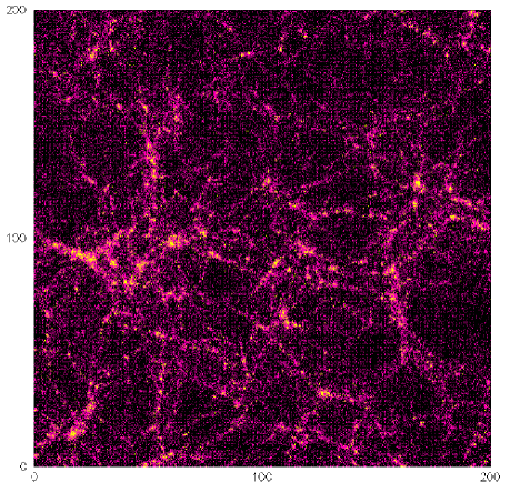
FIG. 10.: A thin slice (26 Mpc/h) of the box (of sides 200 Mpc/h) of the $128^{3},\Lambda$CDM simulation the same as that used for Fig. 6 is shown. Out of the $100,000$ points which have been used for reconstruction more than half are exactly reconstructed. The points which fail exact reconstruction are highlighted (yellow, brighter points). The plot verifies that these points lie mainly in the overdense regions where we do not expect our reconstruction hypothesis to hold well.

Fig. 10 highlights where exact reconstruction fails. We see that exact reconstruction is not achieved in particular in the dense regions. Achieving reconstruction at small scales remains a subject of on-going research. As long as multistreaming effects are unimportant, that is above $\simeq 1$ Mpc, uniqueness of the reconstruction is guaranteed. Approximate algorithms capturing such highly nonlinear effects are now being developed.

VI Conclusion

An accurate reconstruction allows us to test cosmological models by simulating the evolution starting from the reconstructed primordial state and comparing it to observations. Efficient and unique reconstruction would allows us to determine the peculiar velocities of a large number of galaxies, using their positions in redshift catalogues. One could use reconstruction to search for the presence of primordial non-gaussianity and examine the self-consistency of cosmological hypotheses such as the choice of the global cosmological parameters and the assumed biasing scheme. By obtaining a point-by-point reconstruction of the specific realisation that describes the observed patch of our Universe, one could separate the universal properties and the influence of the large-scale environment on the galaxy formation process.

Many previous reconstruction techniques have either suffered from the lack of uniqueness or limited validity which could not be extended beyond the linear Eulerian regime. Our reconstruction scheme overcomes such shortcomings.

We have shown that under suitable hypotheses, there is a unique transformation from the present positions ${\bf x}$ of galaxies (taken as mass tracers) to their respective initial positions ${\bf q}$. Our reconstruction hypothesis first assumes that the Lagrangian map ${\bf x}\rightarrow{\bf q}$ can be written in terms of a potential ${\bf x}={\bf\nabla}_{\bf q}\Phi({\bf q})$. This hypothesis is supported by numerical N-body simulations and is valid up to second order Lagrangian perturbation theory. The second assumption is the convexity of the potential $\Phi({\bf q})$, a consequence of which is the absence of multi-streaming: for almost any Eulerian position, there is a single Lagrangian antecedent. As is well-known, the Zel’dovich approximation leads to caustics and multistreaming. This can be modified in various ways, for example by the introduction of a mock viscosity as is done in the adhesion model (Gurbatov and Saichev 1984, Gurbatov et al. 1989, Shandarin and Zel’dovich 1994). The latter which leads to shocks rather than caustics, is known to have a convex potential (Vergassola et al. 1994) and to be in a better agreement with numerical N-body simulations (Weinberg and Gunn 1990).

By testing our MAK reconstruction against numerical N-body simulations both in real and redshift spaces, we have demonstrated that our reconstruction hypothesis works well down to the scales comparable to the size of collapsed structures, below which the hydrodynamical description of gravitational structure formation ceases to be meaningful (at scales larger than $6$ Mpc/h we achieve more than $62\%$ exact reconstruction). Thus, our reconstruction is rather suitable for large-scale galaxy redshift surveys.

We thank E. Branchini, M. Hénon, J.A. de Freitas Pacheco and P. Thomas for discussions and comments. U.F thanks the Indo-French Center for the Promotion of Advanced Research (IFCPAR 2404-2). A.S. is supported by A CNRS Henri Poincaré fellowship and RFBR 02-01-01062. R.M. is supported by the European Union Marie Curie Fellowship HPMF-CT-2002-01532.

REFERENCES

- [1] Arnold V.I., Mathematical Methods of Classical Mechanics (Springer, Berlin 1978)
- [2] Benamou J.-D. & Brenier Y. 2000, The optimal time-continuous mass transport problem and its augmented Lagrangian numerical resolution, Numer. Math. 84, 375 also at http://www.inria.fr/rrrt/rr-3356.html
- [3] Bertsekas D.P., Network Optimisation: Continuous and Discrete Models (Athena Scientific 1998) Auction algorithm also available at http://web.mit.edu/dimitrib/www/auction.txt
- [4] Bertschinger E. and Dekel A. 1989, ApJ 336, L5
- [5] Branchini E., Nusser A. and Eldar A. 2001, MNRAS 335, 53
- [6] Brenier Y. 1987, C.R.Acad.Sci. 305, 805
- [7] Buchert T. 1992, MNRAS 254, 729
- [8] Burkard R.E. and Derigs U., Assignment and Matching Problems: Solution Methods with FORTRAN-programs, Lecture Notes in Economics and Mathematical Systems No. 184 (Springer, Berlin 1980)
- [9] Catelan P. 1995, MNRAS 276, 115
- [10] Couchman H.M.P., Thomas P.A. and Pearce F.R. 1995, ApJ 452, 797
- [11] Croft R.A. and Gaztañaga 1997, MNRAS 285, 793
- [12] Dekel A., Bertschinger E. and Faber S.M. 1990, ApJ 364, 349
- [13] Frisch U., Matarrese S., Mohayaee R. and Sobolevskii A. 2002, Nature 417, 260
- [14] Gramann, M. 1993, ApJ 405, 449
- [15] Gurbatov S. and Saichev A.I. 1984, Radiophys. Quant. Electr. 27, 303
- [16] Gurbatov S., Saichev A.I. and Shandarin S.F., 1989, MNRAS 236, 385
- [17] Hénon M.A. 1995, C.R.Acad.Sci. 321, 741 A detailed version with the optimisation algorithm is available at http://arxiv.org/abs/math.OC/0209047
- [18] Hjorteland T.,The Action Variational Principle in Cosmology, Thesis, Institute of Theoretical Physics, Univ. of Oslo, June 1999 also available at: http://trond.gothamnights.com/thesis/ Thesis.pdf
- [19] Loveday J., Maddox S.J., Efstathiou G. and Peterson B.A. 1995, ApJ 442, 457
- [20] Monaco P. and Efstathiou G. 1999, MNRAS 308, 763
- [21] Moutarde F., Alimi J.-M., Bouchet F.R., Pellat R. and Ramani A. 1991, ApJ 382, 377
- [22] Munshi D., Sahni V. and Starobinsky 1994, ApJ 436, 517
- [23] Narayanan V.K. and Croft R.A.C. 1999, ApJ 515, 471
- [24] Nusser A. and Branchini E. 2000, MNRAS 313, 587
- [25] Nusser A., Dekel A. Bertschinger E. and Blumenthal G. 1991 ApJ 379, 6
- [26] Nusser A. and Dekel A. 1992 ApJ 391, 443
- [27] Peebles P.J.E. The Large Scale Structure of the Universe (Princeton University Press, 1980)
- [28] Peebles P.J.E. 1989, ApJ L344, 53
- [29] Peebles P.J.E. 1990, ApJ 362, 1
- [30] Sahni V. and Coles P. 1995, Phys. Rept. 262, 1
- [31] Shandarin S.F. and Zel’dovich Y.B. 1989, Rev. Mod. Phys. 61, 185
- [32] Shaya E.J., Peebles P.J.E. and Tully R.B. 1995, ApJ 454, 15
- [33] Taylor A. and Valentine H., 1999, MNRAS 306 491
- [34] Tully R.B., Nearby Galaxies Catalog, Cambridge University Press (Cambridge, UK 1988)
- [35] Valentine H., Saunders W. and Taylor A. 2000, MNRAS 319 L13
- [36] Vergassola M., Dubrulle B., Frisch U. and Noullez A. 1994, A&A 289 325
- [37] Weinberg D.H. and Gunn J.E. 1990, MNRAS 247, 260
- [38] Zel’dovich Y.B. 1970, Astron. & Astrophys. 5, 84