Probing dark energy using baryonic oscillations in the galaxy power spectrum as a cosmological ruler

Abstract

We show that the baryonic oscillations expected in the galaxy power spectrum may be used as a “standard cosmological ruler” to facilitate accurate measurement of the cosmological equation of state. Our approach involves a straight-forward measurement of the oscillation “wavelength” in Fourier space, which is fixed by fundamental linear physics in the early Universe and hence is highly model-independent. We quantify the ability of future large-scale galaxy redshift surveys with mean redshifts $z\approx 1$ and $z\approx 3$ to delineate the baryonic peaks in the power spectrum, and derive corresponding constraints on the parameter $w$ describing the equation of state of the dark energy. For example, a survey of three times the Sloan volume at $z\approx 1$ can produce a measurement with accuracy $\Delta w\approx 0.1$. We suggest that this method of measuring the dark energy powerfully complements other probes such as Type Ia supernovae, and suffers from a different (and arguably less serious) set of systematic uncertainties.

1 Introduction

Measurement of anisotropies in the Cosmic Microwave Background (CMB) radiation have shown the Universe to be (very close to) spatially flat. However, matter only makes up a third of the critical density – the dominant contribution to the energy density of the Universe appears to exist in an unclustered form called “dark energy”. Furthermore, observations of distant supernovae have indicated that the expansion of the Universe has entered a phase of acceleration. This is explicable if dark energy has recently come to dominate the dynamics of the Universe and exerts a large negative pressure. This situation occurs naturally if Einstein’s equations contain a cosmological constant, but the observed magnitude of the vacuum energy is wildly inconsistent with the current predictions of quantum physics. This has motivated the consideration of a more general dark energy equation of state, $P=w\,\rho$ (Turner & White 1997). An accelerating universe is produced if $w<-1/3$ and vacuum energy is described by $w=-1$. If the dark energy is the product of new physics, such as quintessence (e.g. Ratra & Peebles 1988), then the resulting equation of state varies with redshift and must be treated as a more general $w(z)$ (e.g. Linder & Huterer 2003).

Securing more accurate measurements of the dark energy component is of prime cosmological importance. A number of methods have been investigated, most notably the use of Type Ia supernovae as “standard candles” (e.g. Weller & Albrecht 2002). Other possible probes include counts of galaxies (Newman & Davis 2000) and of clusters (Haiman et al. 2001), weak gravitational lensing (Cooray & Huterer 1999), the Alcock-Paczynski test applied to small-scale galaxy correlations (Ballinger et al. 1996) and use of the CMB (e.g. Douspis et al. 2003). In this paper we examine a probe of dark energy that has not received much attention in the literature (e.g. Lahav 2002), but which we believe has many advantages: baryonic oscillations in the galaxy power spectrum.

The CMB power spectrum contains acoustic peaks. Coupling between baryons and photons at recombination imprints these “wiggles” into the matter power spectrum on a scale corresponding to the sound horizon in the early Universe (Peebles & Yu 1970, Eisenstein & Hu 1998). The positions of the peaks and troughs in Fourier space are calculable from straight-forward linear physics and act like a “standard cosmological ruler” (Eisenstein, Hu & Tegmark 1998). Therefore a power spectrum analysis of a galaxy redshift survey containing acoustic oscillations can be used to measure the cosmological parameters (Eisenstein 2002): the conversion of the redshift data into real space requires values of the parameters to be assumed; an incorrect choice leads to a distortion of the power spectrum and the appearance of the acoustic peaks in the wrong places. Standard ruler techniques for deducing the cosmic parameters have been proposed many times before. In the Alcock-Paczynski test (Alcock & Paczynski 1979) a spherical system is distorted into an ellipsoid in the wrong cosmological model. Other examples include the detection of a characteristic clustering scale within the 2dF quasar survey (Roukema, Mamon & Bajtlik 2002) and the use of the angular power spectrum of dark matter haloes (Cooray et al. 2002). Our study is focussed on the ability of the standard ruler provided by the baryonic peaks to measure the dark energy.

Mapping the acoustic peaks in the galaxy power spectrum at high precision, matching those already measured in the CMB power spectrum, would provide a spectacular confirmation of the standard cosmological model in which mass overdensities grow from the seeds of CMB fluctuations. The sharp features of the baryonic oscillations represent a powerful and precise observational test of the current cosmological paradigm (“$\Lambda$-CDM”). Accurate delineation of the baryonic oscillations lies beyond the current state-of-the-art galaxy redshift surveys, the 2dF Galaxy Redshift Survey (Colless et al. 2001) and Sloan Digital Sky Survey (York et al. 2000). Moreover, it is advantageous to place the survey volume at higher redshift (Eisenstein 2002), where the linear regime of galaxy clustering extends to smaller physical scales (unveiling acoustic oscillations to higher spatial frequencies).

In this initial study we present a simple “proof-of-concept” that acoustic oscillations measured at high redshift may be used to accurately determine the dark energy parameter $w$, restricting our attention to cosmological models with constant (redshift-independent) $w$. We perform simulations to quantify the scale of redshift survey required to recover the wiggles and determine the resulting constraints on $w$. We suggest that measurement of the dark energy should be a prime motivation for the next-generation galaxy redshift survey.

2 Measuring baryonic oscillations

In this section we investigate the scale of redshift survey required to measure the acoustic oscillations in the galaxy power spectrum with a specified accuracy.

2.1 Assumptions and approximations

We modelled the baryonic oscillations using the transfer function fitting formulae of Eisenstein & Hu (1998). The matter power spectrum $P(k)$ is deduced from the transfer function $T(k)$ using $P(k)=A\,k^{n}\,T^{2}(k)$; we took the primordial spectral slope to be $n=1$, as (approximately) suggested by inflationary models, and fixed the normalization $A$ such that $\sigma_{8}=1$. The transfer function model is specified by assigning values to the matter density $\Omega_{m}$, the baryon density $\Omega_{b}$ and Hubble’s constant $h=H_{0}/$(100 km s^-1 Mpc^-1). We assumed that it does not depend on the dark energy equation of state: the energy density of dark energy, $\rho_{x}$, relative to that of matter, $\rho_{m}$, scales with redshift as $\rho_{x}/\rho_{m}\propto(1+z)^{3w}$ and is a negligible contributor to physics before recombination (as $w<-1/3$). Of course more complex dark energy models with varying $w$ may lead to significant effects at the epoch of recombination; we do not consider these here, but point out that the CMB is well described by simple matter-dominated models (Spergel et al. 2003). In this section we assume $\Omega_{m}=0.3$, $\Omega_{b}/\Omega_{m}=0.15$, $h=0.7$ and $w=-1$ (i.e. a cosmological constant). Our assumed value for $\Omega_{b}$ is consistent with the latest CMB results (Spergel et al. 2003), constraints from Big Bang nucleosynthesis theory (e.g. O’Meara et al. 2001), and the shape of the galaxy power spectrum measured by the 2dF Galaxy Redshift Survey (Percival et al. 2001). We assume throughout this study that the Universe is flat, $\Omega_{\rm tot}=1$.

The baryonic oscillations can be conveniently displayed by dividing the model $P(k)$ by a smooth reference spectrum containing no wiggles (lower panel of Figure 1; the reference spectrum was obtained from the fitting formulae of Eisenstein & Hu (1998) together with the transfer function). The result is well-approximated by a slowly-decaying sinusoidal function whose peaks are harmonics of the sound horizon scale: approximate formulae for their positions in Fourier space are given by Eisenstein & Hu (1998). The amplitude of the wiggles increases with the baryon density $\Omega_{b}$. The key quantity we wish to observe is the “wavelength” of the acoustic oscillations in $k$-space, which we denote as $k_{A}$, and which is related to the sound horizon at recombination by $k_{A}=2\pi/s$.

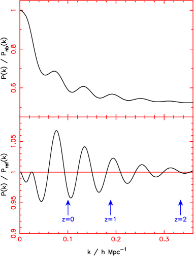
Figure 1: The model power spectrum of Eisenstein & Hu (1998) for cosmological parameters $\Omega_{m}=0.3$, $\Omega_{b}/\Omega_{m}=0.15$, $h=0.7$. For this choice of parameters, the sound horizon $s\approx 105\,h^{-1}$ Mpc and the wiggle wavescale $k_{A}\approx 0.0601\,h$ Mpc^-1. In the upper panel we divide the model $P(k)$ by the corresponding zero-baryon model, $\Omega_{m}=0.3$, $\Omega_{b}=0$, $h=0.7$. Replacing cold dark matter with baryons produces acoustic oscillations and an overall suppression of power. In the lower panel we divide the model $P(k)$ by a smooth fit to the overall shape of the spectrum. The arrows indicate the approximate position of the linear/non-linear transition at different redshifts, estimated in the following way. At $z=0$, we conservatively defined the linear regime by $k<k_{\rm nl}=0.1\,h$ Mpc^-1. From the model $P(k)$ we computed the variance of mass fluctuations $\sigma^{2}(R)$ inside a sphere of radius $R$, where $R=\pi/2k_{\rm nl}$ (i.e. half a fluctuation wavelength, or whole wavecrest, coincides with the diameter $2R$). For $k_{\rm nl}=0.1\,h$ Mpc^-1 we found $\sigma^{2}(\pi/2k_{\rm nl})=0.35$, and then applied this criterion to fix the linear/non-linear transition at other redshifts. At higher $z$, the amplitude of $P(k)$ is reduced by the growth factor, $P(k)\rightarrow P(k)\,D_{1}(z)^{2}$. At $z=1$, for example, $\sigma^{2}(\pi/2k)=0.35$ for $k=0.19\,h$ Mpc^-1 $=k_{\rm nl}(z=1)$. We fixed the overall amplitude of $P(k)$ such that $\sigma^{2}(8\,h^{-1}\,\rm{Mpc})=1$.

If dark energy is neglected at high redshift, the co-moving sound horizon size at last scattering, $s$, is given by (Hu & Sugiyama 1995, Cornish 2001):

$$s=\frac{1}{H_{0}\,\Omega_{m}^{1/2}}\int_{0}^{a_{r}}\frac{c_{s}}{(a+a_{\rm eq})^{1/2}}\,da$$ (1)

where $a_{r}$, $a_{\rm eq}$ are the values of the scale factor $a=1/(1+z)$ at recombination and matter-radiation equality respectively. $c_{s}$ is the speed of sound and is approximately $c/\sqrt{3}$ over the interval of integration. The value of $s$ is of order 100 $h^{-1}$ Mpc.

Thus the theoretical value of $k_{A}$ is set by fundamental CMB physics and depends strongly on $\Omega_{m}$, weakly on $\Omega_{b}$ and negligibly on dark energy. $k_{A}$ is our “standard measuring rod”. In a redshift survey at intermediate redshift $z$, the apparent size of the oscillation wavescale $k_{A}$ will depend on the cosmological geometry, now including the effects of dark energy. As we will see in Section 3, the effects of assuming an incorrect world model (e.g. incorrect $w$) would include a distortion of the measured value of $k_{A}$. (There will be different effects parallel and perpendicular to the line-of-sight, but these are averaged out in our approach). To zeroth order, the precision with which we can empirically measure $k_{A}$ tells us how accurately we can measure the geometrical distance to the redshift $z$ and hence how accurately we can measure the equation of state.

We have assumed that the power spectra of galaxies and of matter are related by a linear bias factor $b$ (where $P_{\rm gal}=b^{2}\,P_{\rm mat}$). Provided our simulated surveys are dominated by sample variance (see Section 2.2), the value of $b$ is unimportant: the fractional error bars $\sigma_{P}/P$ (i.e. the appearance of Figures 1 and 2) do not change if $P(k)$ is scaled by a constant factor (see equation 2). However, increasing the value of $b$ (hence increasing $P_{\rm gal}$) reduces the fractional error due to shot noise, and hence reduces the number of objects required to render shot noise negligible, by a factor $b^{2}$. The assumption of linear bias is simplistic and we plan to include more complicated (redshift-dependent) biassing schemes in a future study.

We scaled the power spectrum to redshift $z$ using the appropriate growth factor, $P(k,z)=P(k,0)\,D_{1}(z)^{2}$. Throughout this paper we use the approximation of Carroll, Press & Turner (1992) for $D_{1}(z)$. This formula is only valid for $w=-1$, but is a satisfactory estimate for models with $w\neq-1$, given that we only treat small departures from $w=-1$ and that we divide out the overall shape of $P(k)$ in the analysis procedure.

These model power spectra are only valid in the linear regime of structure formation; on smaller scales the non-linear growth of structure washes out the baryonic oscillations. At redshift zero, the linear regime only extends to $k\lesssim 0.1\,h$ Mpc^-1 (see Meiksin, White & Peacock 1999, Percival et al. 2001) and perhaps only the first major peak shown in Figure 1 is preserved (i.e. the peak at $k\approx 0.075\,h$ Mpc^-1; there is a small peak predicted at $k\approx 0.025\,h$ Mpc^-1 which is undetectable due to cosmic variance). At higher redshifts ($z\gtrsim 1$) the linear regime extends to much smaller scales, unveiling more acoustic peaks. Moreover, a high-redshift study is necessary to probe dark energy effectively: the conversion of redshifts to spatial scales only depends on the Hubble constant $H_{0}$ at low $z$ and cannot distinguish between different values of $w$.

A galaxy power spectrum deduced from a redshift survey is subject to redshift-space distortions owing to the peculiar velocities galaxies possess on top of the bulk Hubble flow. There are two effects (Kaiser 1987): the coherent infall of galaxies into concentrations of mass (which boosts power on all scales by a constant factor) and the incoherent velocities of galaxies in the central regions of clusters (which damps power on small scales). We make no attempt to simulate these effects. Redshift-space distortions will only produce smooth changes in the shape of the angle-averaged $P(k)$, not sharp features such as acoustic peaks, and we note again that the fractional error bars $\sigma_{P}/P$ do not depend on the absolute value of $P(k)$ (equation 2). In fact, we explicitly divide out the shape using the smooth reference spectrum. Moreover, incoherent velocities do not have an important effect on the large scales probed by acoustic oscillations. These velocities can be modelled by a 1D pairwise dispersion $\sigma_{p}$, and become important on scales $k$ where $k\,\sigma_{p}\gtrsim H_{0}$. At redshift zero, $\sigma_{p}\approx 300$ km s^-1 and power is hence damped on scales $k\gtrsim 0.3\,h$ Mpc^-1. Furthermore, simulations indicate that the value of $\sigma_{p}$ drops by a factor $\sim 2$ between $z=0$ and $z=2$ (Magira, Jing & Suto 2000).

Some models of galaxy clustering (Peacock & Smith 2000, Seljak 2000) predict that the baryonic oscillations in the power spectrum are diluted by a wiggle-free halo contribution (which amounts to a non-local recipe for bias, in which the probability of finding a galaxy is not a simple function of the local mass density). In our initial treatment we assume a standard linear bias factor. However, this should not modify our results to first order: at $z=0$, the halo contribution to the matter power spectrum becomes equal to the linear contribution at $k\approx 0.4\,h$ Mpc^-1 (Peacock & Smith 2000, Figure 2), whereas most of our high-redshift constraining power (all of it in the case of $z\sim 1$) originates from $k<0.2\,h$ Mpc^-1. At higher redshifts the transition in these halo clustering models scales to higher $k$ as described in Smith et al. (2002, Figure 15).

2.2 Back-of-the-envelope calculation

A simple calculation demonstrates that to delineate the oscillations in the galaxy power spectrum accurately, we need to survey a cosmological volume greater than that of the local Sloan Digital Sky Survey (which we take as a uniform cone of $10^{4}$ deg² to $z=0.2$, i.e. $V_{\rm Sloan}=2\times 10^{8}\,h^{-3}$ Mpc³). There are two sources of statistical error in a power spectrum measurement: sample variance (the number of independent wavelengths $2\pi/k$ of a given fluctuation that can fit into the survey volume $V$) and shot noise (the imperfect sampling of fluctuations by the finite number of galaxies $N$).

The error due to sample variance on a power spectrum measurement, averaged over a radial bin in $k$-space of width $\Delta k$, is

$$\left(\frac{\sigma_{P}}{P}\right)^{2}=2\times\frac{(2\pi)^{3}}{V}\times\frac{1}{4\pi k^{2}\Delta k}$$ (2)

(e.g. Peacock & West 1992). This expression is derived from the density of states and the volume of $k$-space enclosed by the radial bin. The initial factor of $2$ is due to the fact that the density field is real rather than complex, thus only half the modes are independent. (For a realistic survey geometry equation 2 is only an approximation, as neighbouring $k$-modes are correlated). Figure 1 indicates that for a statistically significant measurement of the acoustic peak at $k\approx 0.135\,h$ Mpc^-1 we require $\sigma_{P}/P\lesssim 0.02$ as the fractional height of this peak is about 4 per cent. Thus taking $\Delta k=0.015\,h$ Mpc^-1 ($=k_{A}/4$) we find that $V\gtrsim 1.8\,V_{\rm Sloan}$.

The number of galaxies needed to render shot noise negligible in this case is $N\gg 1/P\approx 1\times 10^{5}$ (assuming $b=1$ and using the input model power spectrum to read off $P\times V\approx 5\times 10^{3}\,h^{-3}$ Mpc³ at $k\approx 0.135\,h$ Mpc^-1).

2.3 Simulations

We constructed detailed simulations to determine the scale of survey required to measure the oscillation wavescale $k_{A}$ with a given accuracy. When measuring a power spectrum from a realistic survey, the quantity we derive is actually the power spectrum convolved with the survey window function in $k$-space, $W(k)$, the Fourier transform of the window function in real space. To detect baryonic oscillations it is important that $W(k)$ is compact (non-zero only for $k\ll k_{A}$), otherwise the smoothing effect of the convolution seriously reduces the amplitude of the oscillations. This restricts us to relatively simple survey geometries. (Any remaining convolution has no effect on the observed oscillation wavescale $k_{A}$).

We considered two different potential surveys: the first directed at redshift range $0.5<z<1.3$ and the second probing the range $2.5<z<3.5$. These ranges are reasonable possibilities for future large-scale surveys. The lower-redshift survey could target either luminous star-forming galaxies via 3727Å  [OII] emission, or luminous elliptical galaxies using absorption features such as the 4000Å  continuum break. In either case, $z=1.3$ is a reasonable limit where these spectral features move out of optical wavebands. For the higher redshift survey, the Lyman Break selection technique operates efficiently for $2.5<z<3.5$ as the 912Å  break shifts through the optical $U$-band. Both these redshift regimes have already been explored by small surveys of hundreds of galaxies (e.g. Le Fevre et al. 1995, Steidel et al. 1998) and it is now becoming feasible to extend these efforts to far larger surveys.

For each redshift range $0.5<z<1.3$ and $2.5<z<3.5$ we defined a survey volume $V$ by an angular patch on the sky of size $\theta\times\theta$. We varied the volume $V$ by changing $\theta$ such that $0<V<6\,V_{\rm Sloan}$ in each case ($\theta_{\rm max}=24.9^{\circ}$ and $17.3^{\circ}$ respectively). For the $z\sim 1$ survey we restricted the power spectrum measurements to the Fourier range $k<0.2\,h$ Mpc^-1, which encompasses the first two detectable acoustic peaks. Non-linearities and redshift-space distortions are likely to become important for $k>0.2\,h$ Mpc^-1, diluting the baryonic features. Our estimate of the linear/non-linear transition scale $k_{\rm nl}(z=1)\approx 0.2\,h$ Mpc^-1 is based on using the model power spectrum to calculate the dimensionless variance of mass fluctuations, $\sigma^{2}(R)$, inside a sphere of co-moving radius $R$ equivalent to a fluctuation of wavelength $2\pi/k$. We defined equivalent scales by $R=\pi/2k$, matching a half-wavelength (a full wavecrest) to the diameter $2R$ of the spheres. A conservative estimate of $k_{\rm nl}(z=0)$ is $0.1\,h^{-1}$ Mpc (Meiksin, White & Peacock 1999) which corresponds to $\sigma^{2}(\pi/2k_{\rm nl})=0.35$. At $z=1$, this same value of $\sigma^{2}$ is produced if $k_{\rm nl}\approx 0.2\,h$ Mpc^-1 (see Figure 1). For the $z\sim 3$ survey we extended the measured power spectrum range to $k<0.3\,h$ Mpc^-1, which contains effectively all the visible acoustic peaks. The linear/non-linear transition scale at $z=3$ is $k_{\rm nl}\approx 0.5\,h$ Mpc^-1.

We generated many different Gaussian realizations of $N$ galaxies from the model $P(k)$ within the survey volumes $V$, using Fast Fourier Transform techniques. For simplicity we assumed a constant selection function across the survey volume (i.e. a constant galaxy number density). A more realistic flux-limited survey will detect galaxies with a varying redshift distribution $N(z)$, but optimal weighting techniques for deriving $P(k)$ exist in this case (Feldman, Kaiser & Peacock 1994). We also neglected the evolution of $P(k)$ with redshift over the survey depth, fixing the model power spectrum at the mean redshift of the survey (i.e. $z_{\rm eff}=0.9$ or $z_{\rm eff}=3$). This approximation has a negligible effect on the results as we are only interested in the relative positions of the peaks and troughs in $P(k)$, which are independent of redshift.

For the $z\sim 1$ survey we assumed a linear bias factor $b=1$ for the galaxies. The potential $z\sim 3$ survey will most likely be targetted at Lyman Break galaxies, which are known to be strongly biased tracers of mass (Steidel et al. 1998); in this case we assumed a linear bias parameter $b=3$. As noted above, the main effect of this assumption is to reduce by a factor $b^{2}$ the number of galaxies $N$ required to render shot noise negligible.

We measured the (noisy) power spectrum of each Gaussian realization using the standard method (see e.g. Hoyle et al. 2002). The measurements for the set of realizations allow the statistical error in each spatial frequency bin to be derived, and the ensemble incorporates any correlations that exist between adjacent bins. For each $(N,V)$ simulation we generated 400 realizations. For each realization we divided the measured power spectrum by the smooth reference spectrum and fitted a decaying sinusoidal function to the result, deducing a best-fit oscillation wavescale $k_{A}$ in $k$-space. We permitted the overall amplitude $A$ of the fitted sinusoidal function to vary but fixed the decay rate at an empirically-estimated value, so that we were simply fitting the two-parameter function:

$$\frac{P(k)}{P_{\rm ref}}=1+A\,k\,\exp{\left[-\left(\frac{k}{0.1\,h\,{\rm Mpc}^{-1}}\right)^{1.4}\right]}\,\sin{\left(\frac{2\pi k}{k_{A}}\right)}$$ (3)

The power of $1.4$ in the decay term originates from the Silk damping fitting formula presented in Eisenstein & Hu (1998, equation 21). Varying the decay length as well as the amplitude was found not to have a significant effect on the fitted values of $k_{A}$. For small $k$ there is a phase shift in the sinusoidal term (Eisenstein & Hu 1998, equation 22) but this only affects the acoustic peak at $k\approx 0.025\,h$ Mpc^-1 (see Figure 1) which is not measurable due to sample variance.

For illustration, Figure 2 displays the power spectrum measurement and the best fit of equation 3 for the first realization of the case $z\sim 1$, $V=6\,V_{\rm Sloan}$, $N=2\times 10^{6}$.

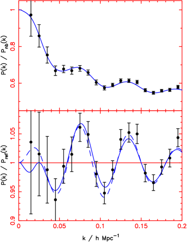
Figure 2: Power spectrum measurement for a simulated survey of $N=2\times 10^{6}$ galaxies over a volume $V=6\,V_{\rm Sloan}$ at redshift $z\sim 1$. The power spectrum is divided by the zero-baryon model in the upper panel and the smooth reference spectrum in the lower panel. The solid line is the input (unconvolved) model power spectrum (i.e. Figure 1). The dashed line in the lower panel is the best fit to the data of a simple decaying sinusoidal function (equation 3). Points are plotted at intervals of $\Delta k=0.01\,h$ Mpc^-1, which are approximately uncorrelated (see Meiksin, White & Peacock 1999).

The distribution of fitted oscillation scales over the different realizations allowed us to describe the accuracy of the measurement by a quantity $\Delta k_{A}/k_{A}$, where $\Delta k_{A}$ is half the range enclosed by the $16^{\rm th}$ and $84^{\rm th}$ percentiles of the distribution (i.e. $k_{A}\pm\Delta k_{A}$ defines the 68 per cent confidence region). Figures 3 and 4 plot contours of the accuracy $\Delta k_{A}/k_{A}$ in the parameter space of $V$ and $N$ for the two potential surveys at $z\sim 1$ and $z\sim 3$. The contours running parallel to the $V-$axis at small $N$ indicate dominance by shot noise; the contours running parallel to the $N-$axis at large $N$ represent dominance by sample variance. The diagonal dashed lines shown in Figures 3 and 4 provide a reasonably good representation of the most efficient observational strategies.

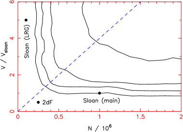
Figure 3: Fractional accuracy $\Delta k_{A}/k_{A}$ with which the wavescale of the baryonic oscillations in $k$-space can be measured at redshift $z\sim 1$, as a function of the number of galaxies $N$ (as a fraction of $10^{6}$) and the survey volume $V$ (as a fraction of the Sloan volume $V_{\rm Sloan}=2\times 10^{8}\,h^{-3}$ Mpc³). Contours are shown corresponding to (beginning in the bottom left-hand corner) $\Delta k_{A}/k_{A}=10\%$, $5\%$, $3\%$ and $2\%$. The positions of the 2dF and Sloan surveys are marked on the plot for comparison. This does not accurately represent their precision in measuring $k_{A}$, because the linear regime at redshift zero extends only to $k\approx 0.1\,h$ Mpc^-1 (whereas the simulations assume $k_{\rm nl}=0.2\,h$ Mpc^-1). Also, the Sloan (LRG) sample will possess a higher linear bias factor $b\approx 1.6$ (whereas the simulations assume $b=1$), which enhances the “effective” value of $N$ by a factor $b^{2}$. Hence the Sloan LRG sample may measure the position of the acoustic peak at $k\approx 0.075\,h$ Mpc^-1 to an accuracy of $\sim 5\%$ (Eisenstein, Hu & Tegmark 1998). The diagonal dashed line indicates the most efficient observational strategies: fewer galaxies will result in shot noise domination, and more galaxies will be “wasted”. The dashed line corresponds to a surface density $\approx 2400$ galaxies deg^-2 in this case.

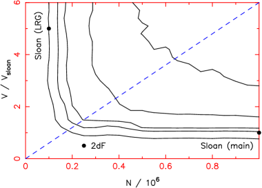
Figure 4: The same plot as Figure 3 for simulated surveys at redshift $z\sim 3$. Note the different scale on the $N-$axis. Contours are shown corresponding to (beginning in the bottom left-hand corner) $\Delta k_{A}/k_{A}=10\%$, $5\%$, $3\%$, $2\%$ and $1.5\%$. The diagonal dashed line corresponds to a surface density $\approx 3400$ galaxies deg^-2.

In order to measure the oscillation wavescale $k_{A}$ with a precision of 2 per cent with negligible shot noise, we require either $\sim 10^{6}$ galaxies covering $\sim 400$ deg² at $z\sim 1$, or $\sim 5\times 10^{5}$ objects over $\sim 150$ deg² at $z\sim 3$. The smaller number of galaxies needed at $z\sim 3$ is due to the larger bias factor $b=3$ which boosts the amplitude of the density fluctuations, more than compensating for the smaller growth factor $D_{1}(z)$. In addition, a given angular field covers more volume at $z\sim 3$ than at $z\sim 1$. However, Lyman Break galaxies will require longer exposure times. The brightest $z\sim 3$ objects of Steidel et al. (1998) typically required $\sim 2$ hours of integration on a 10m telescope to acquire a secure redshift for apparent magnitude $R\sim 24$. An $L^{*}$ galaxy at $z\sim 1$ has brightness $R\sim 23$ and should only require $\sim 30$ minutes exposure.

3 Measuring dark energy with baryonic oscillations

In this section we investigate how accurately a detailed measurement of the baryonic oscillations can constrain the dark energy parameter $w$, which we assume does not vary with redshift. In order to measure $P(k)$ from a galaxy redshift survey we must convert redshifts to co-moving co-ordinates (in $h^{-1}$ Mpc), assuming values for $\Omega_{m}$ and $w$. The expected wiggle wavescale $k_{A}$ is determined by the sound horizon before recombination; it is a function of $\Omega_{m}$, $\Omega_{b}$ and $h$ (see equation 1 or the fitting formula of Eisenstein & Hu 1998, equation 26). Incorrect cosmological parameters will lead to a distortion of the measured power spectrum so that the deduced value of $k_{A}$ is not consistent with the theoretical expectation.

For the purposes of this initial study we assumed that the current values of the matter density and Hubble’s constant are known precisely, $\Omega_{m}=0.3$ and $h=0.7$. We considered a range of values for the baryon density $\Omega_{b}$. To create a concrete example, we assumed a fiducial value $w=-1$ for the dark energy and investigated how accurately we could recover this value from the simulated surveys.

3.1 Back-of-the-envelope calculation

For a flat geometry, the fundamental relation between co-moving distance $x$ and redshift $z$ can be written in the form

$$\frac{dx}{dz}=\frac{c}{H_{0}\,\Omega_{m}^{1/2}}\,\frac{1}{\sqrt{(1+z)^{3}+(\Omega_{m}^{-1}-1)(1+z)^{3(1+w)}}}$$ (4)

For values of $w$ near $-1$, the second term inside the $\sqrt{\ }$ is small for $z\gtrsim 1$ and the zeroth-order dependence is $x\propto H_{0}^{-1}\Omega_{m}^{-1/2}$. This conveniently cancels the zeroth-order dependence of the sound horizon scale on $\Omega_{m}$ and $H_{0}$ in equation 1. Thus our cosmological test has reduced sensitivity to uncertainties in $\Omega_{m}$ and $H_{0}$. We quantify this in Section 4 below.

Suppose $\Omega_{m}=0.3$ and the true dark energy parameter is $w_{true}=-1$. Consider a measuring rod located at $z=1$. If the assumed cosmology is $w_{ass}=-0.9$ (but constant with redshift), then using equation 4 the length distortion of the rod is $dx^{\prime}/dx=0.975$ if oriented radially (i.e. its ends at fixed redshifts) and $x^{\prime}/x=0.980$ if oriented tangentially (i.e. its ends at fixed angular positions). Thus the zeroth order effect is a re-scaling in the length of the rod by $\simeq 2$% and the first order effect is a radial/transverse shear. The full redshift dependence of these quantities is illustrated by Figure 5.

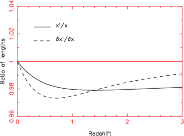
Figure 5: The length distortion of a rod as a function of redshift, supposing the true cosmology is $\Omega_{m}=0.3$, $w_{true}=-1$ and the assumed cosmology is $\Omega_{m}^{\prime}=0.3$, $w_{ass}=-0.9$. The dashed and solid lines illustrate respectively the distortion if the rod is oriented radially (i.e. $dx^{\prime}/dx$) and tangentially (i.e. $x^{\prime}\,d\theta/x\,d\theta=x^{\prime}/x$). Thus it can be seen that the primary effect of assuming an incorrect value of $w$ is a re-scaling of distances away from their true values.

This distortion of spatial scales carries over directly into $k$-space, and suggests that a measurement of $k_{A}$ with 2 per cent precision at $z\sim 1$ translates into a measurement of $w$ with an accuracy $\Delta w\approx 0.1$. The corresponding figures at $z=3$ are $dx^{\prime}/dx=0.991$ and $x^{\prime}/x=0.981$; the smaller distortion in $dx$ suggests that the method is slightly less powerful when applied at $z\sim 3$.

We note that in detail, when combined with CMB observations, the assumption of constant $\Omega_{m}$ in this comparison is not quite right. The CMB power spectrum accurately constrains the angular diameter distance to the surface of last scattering, which removes one degree of freedom in the parameters: we cannot vary $\Omega_{m}$ and a constant $w$ completely independently. In addition, observations by the Planck satellite will accurately determine the quantity $\Omega_{m}h^{2}$ within a few years. However, in this initial treatment, we consider our experiment as independent and suppose that $\Omega_{m}$ is specified by external datasets.

It is interesting to contrast the baryonic oscillations method presented here with the Alcock-Paczynski test. The latter does not employ a standard length-scale known in advance, but rather compares quantities parallel and perpendicular to the line-of-sight. Physically, it is sensitive to distortions in $dx/x$. Numerically, this amounts to the difference between the solid and dashed lines in Figure 5 ($\frac{dx^{\prime}/x^{\prime}}{dx/x}-1\approx\frac{dx^{\prime}}{dx}-\frac{x^{\prime}}{x}$ for small distortions). The baryon wiggles method uses a known ruler and is therefore independently sensitive to distortions in $x$ and $dx$, through the parallel and perpendicular components of the power spectrum (although in this initial treatment we average the power spectrum over angles). Numerically, this is equivalent to the absolute deviation from unity of the solid and dashed lines in Figure 5. Thus the “lever arm” for detecting any departures from $w=-1$ is a factor $\sim 4$ higher at $z=1$ for our method and, in contrast to the Alcock-Paczynski test, it does not depend on small-scale non-linear clustering details.

3.2 Simulations

We simulated surveys in the redshift ranges $0.5<z<1.3$ and $2.5<z<3.5$, as before, using the same measured ranges of $k$ and linear bias factors. In each case we defined the survey volume by a $20^{\circ}\times 20^{\circ}$ angular patch. This generated a volume $V=3.9\,V_{\rm Sloan}$ for the $z\sim 1$ survey and $V=8.0\,V_{\rm Sloan}$ at $z\sim 3$. We assumed redshift catalogues of $N=10^{6}$ galaxies at $z\sim 1$ and $N=5\times 10^{5}$ galaxies at $z\sim 3$, such that the measurements were not limited by shot noise. These examples are somewhat arbitrarily chosen, but are indicative of future large-scale redshift surveys. We selected the galaxies from a redshift distribution that populated the survey volume approximately uniformly.

We allowed the baryon density to vary over the range $0.1<\Omega_{b}/\Omega_{m}<0.2$ (centred on the result $\Omega_{b}/\Omega_{m}=0.15$ assumed in Section 2). For each corresponding power spectrum we generated a set of galaxy realizations and converted these to redshift catalogues supposing a “true” cosmology $w=-1$. We then re-measured $P(k)$ for each realization for a range of “assumed” cosmologies, $-1.3<w<-0.7$. There are some theoretical reasons to suppose $w\geq-1$, but we do not impose this restriction on our analysis (Caldwell 1999).

For each assumed value of $w$ we used 400 different galaxy realizations to derive a distribution of fitted wavescales in $k$-space. If the assumed value of $w$ differs from the “true” cosmology $w=-1$, then the fitted wavescales will be distorted (see Figure 6) and their distribution will not be centred on the expected wavescale (computed from Eisenstein & Hu 1998, equation 26). This allowed us to assign a likelihood to each value of $w$, based on the position of the expected wavescale in the measured distribution. For example, 68 per cent of the fitted wavescales lie between the $16^{\rm th}$ and $84^{\rm th}$ percentiles of the measured distribution. Thus if the expected wavescale lies at the $16^{\rm th}$ percentile of the distribution, the value of $w$ is rejected with “$1\sigma$ significance”. Likewise, if the expected wavescale lies at the $2.5^{\rm th}$ percentile of the distribution, the value of $w$ is rejected with “$2\sigma$ significance”.

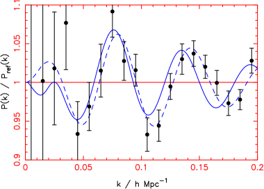
Figure 6: Power spectrum measurement for a simulated survey with the same parameters as Figure 2, except that the value $w=-0.8$ has been incorrectly assumed. The wavescale of the fitted function (the dashed line) is spuriously distorted compared to the theoretical expectation (the solid line).

Figures 7 and 8 display the final results for the $z\sim 1$ and $z\sim 3$ surveys: $1\sigma$ and $2\sigma$ confidence levels for the value of $w$ as a function of $\Omega_{b}$. For the fiducial value of $\Omega_{b}/\Omega_{m}=0.15$ we can indeed measure $w$ to a $1\sigma$ accuracy of $\pm 0.1$, bearing out our back-of-the-envelope calculation in Section 3.1. This of course assumes the fiducial model $w=-1$; the error bar will have some dependence on the “true” value of $w$, which we do not investigate here.

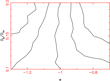
Figure 7: Constraints on the dark energy parameter $w$ produced by measuring the baryonic oscillations in the galaxy power spectrum, for a potential large-scale redshift survey of 400 deg² at $z\sim 1$. We assumed that the linear power spectrum can be successfully measured for $k<0.2\,h$ Mpc^-1. The survey parameters are $V=3.9\,V_{\rm Sloan}$, $N=10^{6}$, $b=1$. We assumed a “true” cosmology $w=-1$ and plot $0\sigma$, $1\sigma$ and $2\sigma$ confidence limits on the measured value of $w$ for varying $\Omega_{b}$. These contours correspond to the theoretical value of $k_{A}$ lying at the $2.5^{\rm th}$, $16^{\rm th}$, $50^{\rm th}$, $84^{\rm th}$ and $97.5^{\rm th}$ percentiles of the observed wavescale distribution. The $50^{\rm th}$ percentile is slightly displaced from $w=-1$ because the full Eisenstein & Hu (1998) transfer function is used in the simulations and the approximate analytic formula (Eisenstein & Hu 1998, equation 26) is used for the theoretical prediction.

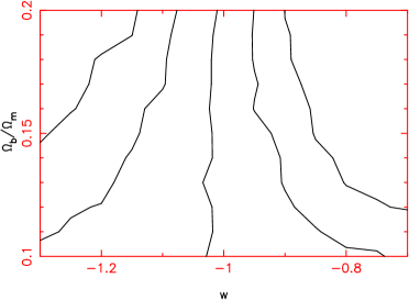
Figure 8: The same plot as Figure 7 for a simulated survey of 400 deg² at $z\sim 3$, supposing that the linear power spectrum can be successfully measured for $k<0.3\,h$ Mpc^-1. The survey parameters are $V=8.0\,V_{\rm Sloan}$, $N=5\times 10^{5}$, $b=3$.

For comparison, we extended the angular area of the simulated $z\sim 1$ survey by a factor of five, generating $N=5\times 10^{6}$ galaxies over a volume $V=30\,V_{\rm Sloan}$. In this case, the wiggle wavescale and dark energy parameter can be measured with respective accuracies $\Delta k_{A}/k_{A}\approx 0.8$ per cent and $\Delta w\approx 0.04$ (assuming $\Omega_{b}/\Omega_{m}=0.15$).

4 Discussion

Baryonic oscillations offer a measurement of the dark energy equation of state that complements other methods. The precision obtainable from the surveys simulated above, $\Delta w\approx 0.1$ ($68$% confidence), is comparable to that achieved by combining together all existing relevant observations. The current high-redshift supernovae data requires $w<-0.55$ at $95$% confidence for a flat geometry (Garnavich et al. 1998), and the latest (WMAP) CMB measurements, taken together with other datasets, imply $w<-0.78$ at $95$% confidence (Spergel et al. 2003). Moreover, if deviations are to be detected from the $w=-1$ paradigm, observations are required at $z\sim 1\rightarrow 3$ where we expect the corresponding cosmological effects to be strongest: Universal expansion switches from deceleration to acceleration at this epoch.

A high-quality sample of 2000 high-redshift supernovae distributed from $z=0.2$ to $z=1.7$, provided by the SNAP satellite (Aldering et al. 2002; http://snap.lbl.gov), promises to measure a constant $w$ to a precision $\Delta w=0.05$ ($68$% confidence) and constrain its time variation. The latter is further improved when combined with the accurate measure of $\Omega_{m}h^{2}$ provided by Planck satellite observations of the CMB (Frieman et al. 2003). The baryon oscillations and supernovae methods of probing the dark energy should powerfully complement each other. Supernovae provide a “standard candle” approach (i.e. a measurement of the luminosity distance), whereas baryon oscillations provide a “standard rod” approach, measuring this rod in both the transverse and radial directions. The transverse rod measures the angular diameter distance. In conventional cosmology and physics, luminosity distance and angular diameter distance are both related to $x(z)$ in equation 4 by $(1+z)$ factors. However, this is not true of all scenarios; for an exotic alternative involving photons oscillating into undetectable light axions see Csáki et al. (2002). The baryonic oscillations additionally measure the standard rod radially, yielding a measurement of $dx/dz$ which is equivalent to the Hubble parameter $H(z)$. To the best of our knowledge the baryonic oscillations provide the only direct route to $H(z)$ at high redshift.

The efficacy of the supernova approach is determined by how accurately systematic errors can be controlled. These systematic astrophysical effects include the possible presence of non-standard host galaxy extinction, the evolution of supernovae with redshift, the effect of gravitational lensing, and variable Milky Way dust extinction. It is important to correct the supernova magnitudes by a light-curve factor (Perlmutter et al. 1997) and/or colour/spectrum factor (Riess et al. 1998). In contrast, the acoustic oscillations method is not limited by systematic errors, but by statistical uncertainties due to sample size.

The two approaches also differ in their requirement of a local calibration. In the supernova method, cosmological parameters follow from the relative brightnesses of supernovae at different redshifts: hence the Nearby Supernova Factory (http://snfactory.lbl.gov) plans a detailed study of several hundred low-redshift supernovae. In contrast, the measuring-rod length for the acoustic peaks is given directly by fundamental physics ($\Omega_{m}h^{2}$ and $\Omega_{b}h^{2}$) and does not require additional observations at $z=0$.

The use of counts of galaxies or clusters as probes of dark energy also depends on understanding critical systematics such as the variation with redshift of the intrinsic number density of the objects, and the ability to identify systems of comparable mass at different redshifts.

The approach presented here is essentially a geometrical method, similar in conception to the Alcock-Paczynski test. A classic application of the Alcock-Paczynski test is to small-scale galaxy clustering parallel and perpendicular to the line-of-sight (Ballinger et al. 1996). However, in this case it is very difficult to distinguish the geometrical distortions imprinted by an incorrect cosmology from redshift-space distortions. In contrast, baryonic oscillations probe clustering on much larger scales, where redshift-space distortions are insignificant.

In our very empirical approach, the measurement of $w$ depends only on knowledge of the positions of the acoustic peaks and troughs in the power spectrum (and not on the detailed shape and amplitude of the power spectrum). It is the positions of these peaks, our “standard rod”, which are the least model-dependent aspects of the power spectrum. Detailed models exist for physics before recombination, tested by increasingly accurate observations of the CMB power spectrum. The subsequent physics governing the growth of structures lies firmly in the well-understood linear regime for the scales of interest.

However, three important issues have been ignored in this initial investigation and will be considered in a future study (see also Seo & Eisenstein, in prep.). The most important unexplored effect in the use of baryonic oscillations is the possible existence of more complicated galaxy biassing schemes (a non-linear bias that may evolve with redshift). This said, linear scale-independent bias should not be a bad approximation on large scales (e.g. Peacock & Dodds 1994). Secondly, we have restricted our attention to models with a constant, redshift-independent value of $w$. Our approach can be simply extended to constrain models of varying $w$, such as the common parameterizations $w(z)=w_{0}+w_{1}\,z$ or $w(z)=w_{0}+w_{a}\,z/(1+z)$ which will be the subject of a future study. Thirdly, we have neglected the uncertainty in the value of $\Omega_{m}$, which clouds precise knowledge of the expected positions of the acoustic peaks.

It is easy to estimate the implications of uncertainty in $\Omega_{m}$ for our method, assuming a “true” cosmology $\Omega_{m}=0.3$, $w=-1$. We saw in Section 3.1 that a shift $\Delta w=0.1$ produces a radial distortion (in $dx/dz$) of $\approx 2$ per cent at $z=1$. Using equation 4, a similar distortion is produced by a shift $\Delta\Omega_{m}\approx 0.02$. However, the sound horizon is also changed by $\approx 1.5$ per cent in the same sense (using the fitting formula of Eisenstein & Hu 1998, equation 26), thus the effects largely cancel out. The “overall” radial distortion (relative to the sound horizon) becomes 2 per cent when $\Delta\Omega_{m}\approx 0.07$, which is reassuring: combining the WMAP CMB results with other astronomical data sets produces a current measurement of $\Omega_{m}$ with accuracy $\Delta\Omega_{m}\approx 0.04$ (Spergel et al. 2003), and this situation should improve in the light of new data. However, the $z\sim 3$ survey demands much tighter knowledge of $\Omega_{m}$ than the $z\sim 1$ survey, because the $(1+z)^{3}$ term inside the $\sqrt{\ }$ in equation 4 starts heavily winning and the distortion due to a shift in $w$ decreases. The result is that at $z=3$, the shift $\Delta\Omega_{m}\approx 0.01$ produces the same overall radial distortion as $\Delta w=0.1$. Thus the application of this method at $z=3$ requires more accurate knowledge of $\Omega_{m}$ than is achievable from current data.

It is worth considering whether an imaging survey using photometric redshifts could accurately measure the acoustic peaks (see also Eisenstein 2002). Let us introduce a Gaussian scatter $\sigma_{z}=(1+z)\sigma_{0}$ in each galaxy redshift. This corresponds to a smearing in co-moving co-ordinates of magnitude $\sigma_{r}=\sigma_{z}(dx/dz)$. Taking a concrete example, if $\sigma_{0}=0.03$ (a realistic estimate of the best possible current accuracy of photometric redshifts, e.g. Wolf et al. 2003) then $\sigma_{r}\approx 100\,h^{-1}$ Mpc at $z=1$. The effect on a spherically symmetric $P(k)$ in ($k_{x}$,$k_{y}$,$k_{z}$)-space is a damping of all modes by a factor $\exp{(-k_{z}^{2}\sigma_{r}^{2})}$ (in the flat-sky approximation), where the $z$-axis is the line-of-sight. Considering the modes in a spherical shell of radius $k=0.2\,h$ Mpc^-1, the majority are too heavily damped to provide signal. The surviving useful modes (with $|k_{z}|<1/\sigma_{r}\approx 0.01\,h$ Mpc^-1) are located within a “ring” in $k$-space, corresponding to a reduction in the number of useful modes by a factor $k\sigma_{r}\approx 20$. To achieve the same power spectrum precision on this scale $k$, the sky area of the imaging survey (i.e. density of states in $k$-space) must be increased by this same factor $\approx 20$ such that the ring contains the same number of modes as the original spherical shell.

However, the most significant disadvantage of the photometric redshifts approach is one loses the capacity to decompose the power spectrum into its radial and tangential components, which separately constrain the Hubble constant and angular diameter distance through distortions in $dx$ and $x$ (Eisenstein 2002). In our initial “proof-of-concept” treatment, we have averaged the power spectrum over angles and not pursued these separate constraints, which certainly merit more detailed calculation (see Seo & Eisenstein, in prep.). As noted above, the radial component of $P(k)$ is damped by a factor $\exp{(-k^{2}\sigma_{r}^{2})}$, which becomes unacceptably small unless $\sigma_{r}\lesssim 1/k$ or (taking $k=0.2\,h$ Mpc^-1) $\sigma_{0}\lesssim 0.001$ at $z=1$. Spectroscopic resolution $R\sim 1000$ is thus required for sufficiently accurate redshifts.

Finally, how realistic is it to carry out such redshift surveys in practice? Our simulated surveys involve $\sim 10^{6}$ galaxies over $\sim 400$ deg² of sky. The exposure times for spectra of these objects would be of order 1–2 hours on 8-metre class telescopes, based on existing data (e.g. Steidel et al. 1998). An 8-metre telescope with a $1^{\circ}$ diameter field of view, capable of taking spectra of up to 3000 galaxies simultaneously, could accomplish such a survey in 60–120 nights. Such an instrument is eminently feasible and has been proposed several times (Glazebrook 2002). In particular, a detailed concept design has been put together for the Gemini telescopes (Barden 2002). The observing time and data volume of such a survey is very similar to that of the 2dF Galaxy Redshift Survey (Colless et al. 2001).

5 Conclusions

This initial study has demonstrated that, under a simple set of assumptions, baryonic oscillations in the galaxy power spectrum may be used to measure accurately the equation of state of the dark energy. For example, a survey of three times the Sloan volume at mean redshift $z\sim 1$ can measure the sound horizon (i.e. the wiggle scale) with an accuracy of 2 per cent, and the parameter $w$ (assumed constant) with precision $\Delta w=0.1$, assuming $\Omega_{b}/\Omega_{m}=0.15$. This probe of the dark energy is complementary to the supernova method, with an entirely different set of uncertainties dominated by sample size rather than systematic effects. It would provide the second independent pillar of evidence for the current epoch acceleration of the Universal expansion. The constraints on $w$ become tighter as the survey volume is enlarged. We conclude that delineation of the baryonic peaks, and their use as a standard cosmological ruler to constrain cosmological parameters, should form an important scientific motivation for the next generation of galaxy redshift surveys.

References

- (1) Alcock C., Paczynski B., 1979, Nature, 281, 358
- (2) Aldering G. et al., 2002, SPIE, 4835, in press (astro-ph/0209550)
- (3) Ballinger W.E., Peacock J.A., Heavens A.F., 1996, MNRAS, 282, 877
- (4) Barden S., 2002, in “Next Generation Wide-Field Multi-Object Spectroscopy”, ASP Conference Series vol. 280, ed. M.Brown & A.Dey
- (5) Caldwell R.R., 1999, Phys.Lett.B, 545, 23
- (6) Carroll S.M., Press W.H., Turner E.L., 1992, ARA&A, 30, 499
- (7) Colless M. et al., 2001, MNRAS, 328, 1039
- (8) Cooray A.R., Huterer D., 1999, ApJ, 513, 95
- (9) Cooray A.R., Hu W., Huterer D., Joffre M., 2001, ApJ, 557, 7
- (10) Cornish N.J., 2001, PhRvD, 63, 7302
- (11) Csáki C., Kaloper N., Terning J., 2002, Physical Review Letters, 88, 161302
- (12) Douspis M., Riazuelo A., Zolnierowski Y., Blanchard A., 2003, A&A, submitted (astro-ph/0212097)
- (13) Eisenstein D.J., 2002, “Large-scale structure and future surveys” in “Next Generation Wide-Field Multi-Object Spectroscopy”, ASP Conference Series vol. 280, ed. M.Brown & A.Dey (astro-ph/0301623)
- (14) Eisenstein D.J., Hu W., 1998, ApJ, 496, 605
- (15) Eisenstein D.J., Hu W., Tegmark M., 1998, ApJ, 504, 57
- (16) Feldman H.A., Kaiser N., Peacock J.A., 1994, ApJ, 426, 23
- (17) Frieman J.A., Huterer D., Linder E.V., Turner M.S., 2003, PhRvD, submitted (astro-ph/0208100)
- (18) Garnavich P.M. et al., 1998, ApJ, 509, 74
- (19) Glazebrook K., 2002, “Achieving high-object multiplex in future wide field spectroscopic surveys” in “Next Generation Wide-Field Multi-Object Spectroscopy”, ASP Conference Series vol. 280, ed. M.Brown & A.Dey
- (20) Haiman Z., Mohr J.J., Holder G.P., 2001, ApJ, 553, 545
- (21) Hoyle F., Outram P.J., Shanks T., Croom S.M., Boyle B.J., Loaring N.S., Miller L., Smith R.J., 2002, MNRAS, 329, 336
- (22) Hu W., Sugiyama N., 1995, ApJ, 444, 489
- (23) Kaiser N., 1987, MNRAS, 227, 1
- (24) Lahav O., 2002, “Could dark energy be measured from redshift surveys?” in the XVIIIth IAP meeting “On the Nature of Dark Energy” (astro-ph/0212358)
- (25) Le Fevre O., Crampton D., Lilly S.J., Hammer F., Tresse L., 1995, ApJ, 455, 60
- (26) Linder E.V., Huterer D., 2003, PhRvD, submitted (astro-ph/0208138)
- (27) Magira H., Jing Y.P., Suto Y., 2000, ApJ, 528, 30
- (28) Meiksin A., White M., Peacock J.A., 1999, MNRAS, 304, 851
- (29) Newman J.A., Davis M., 2000, ApJL, 534, 11
- (30) O’Meara J.M., Tytler D., Kirkman D., Suzuki N., Prochaska J.X., Lubin D., Wolfe A.M., 2001, ApJ, 552, 718
- (31) Peacock J.A., Dodds S.J., 1994, MNRAS, 267, 1020
- (32) Peacock J.A., Smith R.E., 2000, MNRAS, 318, 1144
- (33) Peacock J.A., West M.J., 1992, MNRAS, 259, 494
- (34) Peebles P.J.E., Yu J.T., 1970, ApJ, 162, 815
- (35) Percival W.J. et al., 2001, MNRAS, 327, 1297
- (36) Perlmutter S. et al., 1997, ApJ, 483, 565
- (37) Ratra B., Peebles P.J.E., 1988, PhRvD, 37, 3406
- (38) Riess A. et al., 1998, AJ, 116, 1009
- (39) Roukema B.F., Mamon G.A., Batjlik S., 2002, A&A, 382, 397
- (40) Seljak U., 2000, MNRAS, 318, 203
- (41) Seo H., Eisenstein D.J., in preparation
- (42) Smith R.E. et al., 2002, MNRAS, submitted (astro-ph/0207664)
- (43) Spergel D.N. et al., 2003, ApJ submitted (astro-ph/0302209)
- (44) Steidel C.C., Adelberger K.L., Dickinson M., Giavalisco M., Pettini M., Kellogg M., 1998, ApJ, 492, 428
- (45) Turner M.S., White M., 1997, PhRvD, 56, 4439
- (46) Weller J., Albrecht A., 2002, PhRvD, 65, 3512
- (47) Wolf C., Meisenheimer K., Rix H.-W., Borch A., Dye S., Kleinheinrich M., 2003, A&A, 401, 73
- (48) York D.G. et al., 2000, AJ, 120, 1579