The Detectability of the First Stars and Their Cluster Enrichment Signatures

Abstract

We conduct a comprehensive investigation of the detectability of the first stars and their enrichment signatures in galaxy clusters. As the initial mass function (IMF) of these Population III (PopIII) stars is unknown, and likely to be biased to high masses, we base our study on analytical models that parameterize these uncertainties and allow us to make general statements. We show that the mean metallicity of outflows from PopIII objects containing these stars is well above the critical transition metallicity ($Z_{\rm cr}\sim 10^{-4}Z_{\odot}$) that marks the formation of normal stars. Thus the fraction of PopIII objects formed as a function of redshift is heavily dependent on the distribution of metals and fairly independent of the mean metallicity of the universe, or the precise value of $Z_{\rm cr}.$

Using an analytic model of inhomogeneous structure formation, we study the evolution of PopIII objects as a function of the star formation efficiency, IMF, and efficiency of outflow generation. For all models, PopIII objects tend to be in the $10^{6.5}{M_{\odot}}-10^{7.0}{M_{\odot}}$ mass range, just large enough to cool within a Hubble time, but small enough that they are not clustered near areas of previous star formation. Although the mean metallicity exceeds $Z_{\rm cr}$ at $z\sim 15$ in all models, the peak of PopIII star formation occurs at $z\sim 10$ and such stars continue to form well into the observable range. We discuss the observational properties of these objects, some of which may have already been detected in ongoing surveys of high-redshift Lyman-$\alpha$ emitters.

Finally, we combine our PopIII distributions with the yield models of Heger and Woosley (2002) to study their impact on the intracluster medium (ICM) in galaxy clusters. We find that PopIII stars can contribute no more than 20% of the iron observed in the ICM, but if they form with characteristic masses $\sim 200-260{M_{\odot}}$, their peculiar elemental yields help to reconcile theoretical models with the observed Fe and Si/Fe abundances. However, these stars tend to overproduce S/Fe and can account only for the O/Fe ratio in the inner regions of poor clusters. Additionally, the associated SN heating falls far short of the observed level of $\sim 1{\rm keV}$ per ICM gas particle. Thus the properties of the first objects may be best determined by direct observation.

1. Introduction

The properties of the first cosmic stars born out of a primordial, metal-free gas may have been quite different from those of later generations formed from polluted material. Studies of the gravitational collapse of the $10^{6-7}M_{\odot}$ pre-galactic units that harbor the first stars suggest that these Population III (PopIII) objects fragmented into clumps with typical masses of $10^{3-4}M_{\odot}$ (Abel et al. 1998; Bromm, Coppi, & Larson 1999, 2002; Abel, Bryan & Norman 2000; Bromm et al. 2001) that did not subdivide further (Omukai & Nishi 1998; Nakamura & Umemura 1999; Ripamonti et al. 2002). As the strong accretion rates (up to 0.1 $M_{\odot}\mbox{yr}^{-1}$) onto the central protostellar cores in these clumps could not have been arrested by radiation pressure, bipolar outflows, rotation or by any other known mechanism (Ferrara 2001), they are likely to have evolved into very massive stars. Such massive star formation mode would have continued until the gas metallicity passed a critical threshold of $Z_{\rm cr}\lower 2.15277pt\hbox{$\;\buildrel<\over{\sim}\;$}10^{-4}Z_{\odot}$ (Omukai 2000; Bromm et al. 2001; Schneider et al. 2002), which enabled both the formation of lower mass clumps and some of the above mechanisms to stop accretion.

This situation leads to the so-called star formation conundrum pointed out in Schneider et al. (2002). If PopIII stars were indeed very massive $M_{\star}\geq 100M_{\odot}$, stellar evolution models predict that most of these objects would have evolved into black holes, which lock in their nucleosynthetic products. This in turn would prevent the metal enrichment of the surrounding gas and force the top-biased star formation mode to continue indefinitely. It is only in a relatively narrow mass window in fact, $\Delta_{\gamma\gamma}\equiv 140{M_{\odot}}\leq M_{\star}\leq 260{M_{\odot}}$, that ejection of heavy elements can occur, powered by so called pair-instability supernovae in which a pair-production instability ignites explosive nucleosynthesis. Thus these supernovae may be essential to increase the intergalactic medium (IGM) metallicity above $Z_{\rm cr}$ and initiate the transition from top-biased star formation to the formation of “normal” (PopII/PopI) stars with a more typical initial mass function (IMF).

While this transition must have occurred at high redshift in the bulk of cosmic star formation sites (as suggested by the predicted diffuse neutrino flux associated to the black hole collapse of the first stars, Schneider, Guetta, & Ferrara 2002, and by the interpretation of the near infrared background, Salvaterra & Ferrara 2003) massive PopIII stars are likely to have left some imprints that are observable today. One point that might have important observational consequences is the fact that cosmic metal enrichment has proceeded very inhomogeneously (Scannapieco, Ferrara, & Madau 2002; Thacker, Scannapieco, & Davis 2002; Furlanetto & Loeb 2002), with regions close to star formation sites rapidly becoming metal-polluted and overshooting $Z_{\rm cr}$, and others remaining essentially metal-free. Thus, the two modes of star formation, PopIII and normal, must have been active at the same time and possibly down to relatively low redshifts, opening up the possibility of detecting PopIII stars.

This is particularly important as metal-free stars are yet to be detected. This could be attributed to a statistical paucity of metal-free stars or may be due to their absence entirely, hinting at short-lived, massive first stars. At the same time, theoretical studies are making rapid progress in understanding the radiative properties (Tumlinson, Giroux, & Shull 2001; Bromm, Kudritzki, & Loeb 2001) and spectral energy distributions of such stars (Schaerer & Pelló 2002; Oh, Haiman, & Rees 2001), and their interactions with the ambient medium (Ciardi & Ferrara 2001). Thus, it might well be that the best approach to detect the first stellar clusters is to develop careful observation strategies of high-redshift PopIII host candidates. This is the first aspect that we investigate in detail in this paper.

However, direct observations are not the only way to learn about the first cosmic stars. Abundance patterns measured in different cosmic objects may already show clear imprints of such early star formation. A prime example are observations of metal-poor halo stars. Although these stars cannot be the massive PopIII stars themselves, they might be old enough to retain some record of the metals ejected by the first stellar generation (Cayrel 1996; Weiss et al. 2000). Indeed, high-resolution spectroscopy of metal poor-halo stars has uncovered a number of unusual abundance patterns in the iron peak elements in stars with [Fe/H]$\sim-2.5$ (McWilliam et al. 1995; Ryan et al. 1996). In these stars the mean values of [Cr/Fe] and [Mn/Fe] decrease toward smaller metallicities, [Co/Fe] increases with metallicity, and r- and s-process elements are nearly absent: trends that cannot be interpreted with Type II or Type Ia SNa yields (Oh et al. 2001; Umeda & Nomoto 2002). Very recently, the Hamburg/ESO objective prism survey (HES) team has reported the discovery of a star HE0107-5240 with a mass of $0.8{M_{\odot}}$ and an iron abundance of [Fe/H] = $-5.3\pm 0.2$ (Christlieb et al. 2002). While this iron value is uniquely low, the overall metallicity of this star is within the estimated range for $Z_{\rm cr}$ ($10^{-6}Z_{\odot}<Z_{\rm cr}\leq 10^{-4}Z_{\odot}$, Schneider et al. 2002, 2003) suggesting that the identification of more stars with iron abundances less than [Fe/H]$<-5$ will be extremely important to elucidate the conditions that enable low-mass star formation.

A second indirect approach is to search for PopIII enrichment in the intergalactic medium itself. Tremendous progress has been made recently in the determination of the metal content of the IGM both observationally (Ellison et al. 2000; Schaye et al. 2000; Songaila 2001) and theoretically (Gnedin & Ostriker 1997; Ferrara, Pettini, & Shchekinov 2000; Cen & Bryan 2001; Scannapieco & Broadhurst 2001; Madau, Ferrara, & Rees 2001; Scannapieco, Ferrara, & Madau 2002; Thacker, Scannapieco, & Davis 2002; Furlanetto & Loeb 2002). However, abundance patterns in the low-column density Ly$\alpha$ forest can be obtained only for a few elements and are complicated by uncertain ionization corrections.

In this work, we examine a third possibility for searching for signatures of PopIII star formation, by studying the intracluster medium (ICM). Metal abundance experiments are easier in the ICM than in the more diffuse IGM due not only to higher gas densities, but to the lower redshift of the targets, the simpler physics of the collisionally ionized gas, and the larger statistics. Such an approach parallels similar efforts by Renzini (1999) and Loewenstein (2001), but it is specifically designed to test for PopIII star formation.

The properties of ICM may also provide information as to the energetics of SN_γγ , whose high energy output is suggestive of well-know entropy-floor problem (Loewenstein 2000; Lloyd-Davies, Ponman, & Cannon 2000; Tozzi & Norman 2001; Borgani et al. 2001). Here a wide range of observations have shown that ICM is much more diffuse and extended than predicted by simple virialization models, resulting in an X-ray luminosity-temperature relation that is widely discrepant with simple predictions (Kaiser 1991). This discrepancy appears to be due to a baseline entropy of $55-110~{}h^{-1/3}$ keV cm², where this uncertainty is due to the unknown extent to which shocks have been suppressed in low-mass systems. This excess appears to be distributed uniformly with radius outside the central cooling regions and provides an additional constraint on our models of PopIII formation.

Our aim is hence twofold. We first investigate the spatial distribution and redshift evolution of galaxies hosting PopIII stars. This study enables us to predict a number of observationally related quantities (detection probabilities, number counts, equivalent width distributions) that we combine into a search strategy to find these systems. Secondly, we turn to the effects of these metal-free stars on the metallicity patterns and energetics of galaxy clusters.

Throughout this paper, we restrict our attention to a cosmological model in which $h=0.65$, $\Omega_{M}$ = 0.3, $\Omega_{\Lambda}$ = 0.7, $\Omega_{b}=0.05$, $\sigma_{8}=0.87$, $\Gamma=0.18,$ and $n=1$, where $h$ is the Hubble constant in units of 100 km s^-1 Mpc^-1, $\Omega_{M}$, $\Omega_{\Lambda}$, and $\Omega_{b}$ are the total matter, vacuum, and baryonic densities in units of the critical density, $\sigma_{8}$ is the mass variance of linear fluctuations on the $8h^{-1}{\rm Mpc}$ scale, $\Gamma$ is the CDM shape parameter, and $n$ is the tilt of the primordial power spectrum. The choice of these parameters is based mainly on measurements of Cosmic Microwave Background anisotropies (eg. Balbi et al. 2000; Netterfield et al. 2002; Pryke et al. 2002) and the abundance of galaxy clusters (eg. Viana & Liddle 1996).

The structure of this work is as follows. In §2 we derive metal yields and kinetic energy input from pair-creation and Type II SNe, and in §3 we use these quantities to construct a model of metal dispersal by SN-driven outflows. In §4 we present an analytic model of inhomogeneous structure formation which we use in §5 to estimate the distribution of cosmic objects hosting PopIII or PopII/I stars, accounting for feedback effects due to outflows pre-enriching neighboring halos. In §6 we apply these results to construct the Lyman-$\alpha$ flux and redshift distribution of PopIII objects and discuss strategies for their direct detection. In §7 we turn our attention to the intracluster medium of galaxy clusters, and relate the thermal and enrichment properties of this gas to the properties of PopIII objects. Conclusions are given in §8.

2. Metal Yields and Explosion Energies

In order to quantify the properties of PopIII and PopII/I objects, we consider the metal yields and explosion energies of pair-creation (SN_γγ) and Type II SNe (SNII), respectively. In the PopII/I case we adopt the results of Woosley & Weaver (1995) who compute these quantities for SNII as a function of progenitor mass in the range $12{M_{\odot}}<M_{\star}<40{M_{\odot}}$ and initial metallicities $Z=(0,10^{-4},10^{-2},10^{-1},1)~{}Z_{\odot}$. The corresponding quantities for SN_γγ are taken from Heger & Woosley (2002) assuming progenitors in the mass range $\Delta_{\gamma\gamma}\equiv 140{M_{\odot}}\leq M_{\star}\leq 260{M_{\odot}}$.

2.1. PopII/I Objects

The total heavy-element mass and energy produced by a given object depend on the assumed IMF. We define PopII/I objects as those that host predominantly PopII/PopI stars, i.e. objects with initial metallicity $Z\geq Z_{\rm cr}=10^{-4}Z_{\odot}$. For these, we assume a canonical Salpeter IMF, $\Phi(M)\propto M^{-(1+x)}$, with $x=1.35$, and lower (upper) mass limit $M_{l}=0.1{M_{\odot}}$ ($M_{u}=100{M_{\odot}}$), normalized so that,

$$\int_{M_{l}}^{M_{u}}dMM\Phi(M)=1.$$ (1)

The IMF-averaged SNII metal yield of a given heavy element $i$ (in solar masses) is then

$$Y_{i}^{II}\equiv\frac{\int_{\small M_{SNII}}^{\small M_{BH}}dM\Phi(M)M_{i}}{\int_{\small M_{SNII}}^{\small M_{BH}}dM\Phi(M)}$$ (2)

where $M_{i}$ is the total mass of element $i$ ejected by a progenitor with mass $M$. The mass range of SNII progenitors is usually assumed to be $(8-100){M_{\odot}}$. However, above $M_{BH}=50\pm 10{M_{\odot}}$ stars form black holes without ejecting heavy elements into the surrounding medium (Tsujimoto et al. 1995), and from $(8-11){M_{\odot}}$ the pre-supernova evolution of stars is uncertain, resulting in tabulated yields only between $12{M_{\odot}}$ and $40{M_{\odot}}$ (Woosley & Weaver 1995). To be consistent with previous investigations (Gibson, Loewenstein, & Mushotzky 1997; Tsujimoto et al. 1995), in our reference model (SNII-C in Table 1) we consider SNII progenitor masses $M_{SNII}=10{M_{\odot}}\leq M_{\star}\leq M_{BH}=50{M_{\odot}}$ range, linearly extrapolating from the lowest and highest mass grid values. Finally, SNII yields depend on the initial metallicity of the progenitor star. Here we assume for simplicity that SNII progenitors form out of a gas with $Z\geq 10^{-2}Z_{\odot}$. This choice is motivated by the typical levels of pre-enrichment from PopIII stars (see Section 3). Moreover, the predicted SNII yields with initial metallicity in the range $10^{-4}Z_{\odot}\leq Z\leq 10^{-2}Z_{\odot}$ are largely independent of the initial metallicity of the star (Woosley & Weaver 1995). Different combinations of progenitor models relevant for the present analysis are illustrated in Table 1. The last entry in each row is the number of SNII progenitors per unit stellar mass formed,

$${\cal N}^{II}\equiv\frac{\int_{\small M_{SNII}}^{\small M_{BH}}dM\Phi(M)}{\int_{\small M_{l}}^{\small M_{u}}dMM\Phi(M)}.$$ (3)

Finally, we assume that each SNII releases ${\cal E}_{\rm kin}=1.2\times 10^{51}$ erg, independent of the progenitor mass (Woosley & Weaver 1995).

Table 1The different progenitor models for SNII. The masses are in ${M_{\odot}}$ and ${\cal N}^{II}$ is in units of ${M_{\odot}}^{-1}$.

SN Model	$M_{SNII}$	$M_{BH}$	$Z/Z_{\odot}$	${\cal N}^{II}$
SNII-A	12	40	$10^{-2}$	0.00343
SNII-B	12	40	1	0.00343
SNII-C	10	50	$10^{-2}$	0.00484
SNII-D	10	50	1	0.00484

Table 2SN_γγ Progenitor models. The first three entries are in ${M_{\odot}}$, $\,\,{\cal N}^{\gamma\gamma}$ is in units ${M_{\odot}}^{-1}$ and ${\cal E}_{\rm kin}$ is in units of $10^{51}$ erg. The last entry represents the kinetic energy per unit gas mass, ${\cal E}^{III}_{\rm g}=f^{III}_{*}f_{w}{\cal N}^{\gamma\gamma}{\cal E}^{III}_{\rm kin}$ in units of $10^{51}$ erg ${M_{\odot}}^{-1}$ computed assuming $f^{III}_{*}=0.1$ and $f_{w}=0.1$ (see text).

SN Model	$M_{C}$	$\sigma_{C}^{\rm min}$	$\sigma_{C}^{\rm max}$	${\cal N}^{\gamma\gamma}$	$f_{\gamma\gamma}$	${\cal E}^{III}_{\rm kin}$	${\cal E}^{III}_{\rm g}$
SNγγ -A	100	10	17	$<6\times 10^{-5}$	$[0.03-8]10^{-3}$	$6-7.5$	$<4\times 10^{-6}$
SNγγ -B	200	20	50	$[5-4]10^{-3}$	$0.99-0.8$	$38.4-37.5$	$[2-1.5]10^{-3}$
SNγγ -C	260	26	70	$[2.1-2.2]10^{-3}$	$0.5-0.4$	$67.1-46.4$	$[1.4-1]10^{-3}$
SNγγ -D	300	30	83	$[0.4-1.4]10^{-3}$	$0.09-0.3$	$70.5-48.2$	$[2.6-6.6]10^{-4}$
SNγγ -E	500	50	149	$<2.2\times 10^{-4}$	$<0.05$	$70.6-47.8$	$<10^{-4}$
SNγγ -F	1000	100	314	$<3\times 10^{-5}$	$<6.3\times 10^{-3}$	$69.9-43.6$	$1.3\times 10^{-5}$

Table 3The IMF-averaged metal yields (in ${M_{\odot}}$) for SNII, SNIa, and SN_γγ .

SN Model	$Y_{\rm O}$	$Y_{\rm Si}$	$Y_{\rm S}$	$Y_{\rm Fe}$	$Y_{\rm met}$
SNII-A	1.43	0.133	0.064	0.136	2.03
SNII-B	1.56	0.165	0.078	0.115	2.23
SNII-C	1.11	0.1	0.047	0.126	1.6
SNII-D	1.19	0.124	0.061	0.11	1.76
SNIa	0.148	0.158	0.086	0.744	1.23
SNγγ -A	48.4-47.5	2.07-4.37	0.559-13.2	$[0.29-13.3]10^{-2}$	59.3 - 61.3
SNγγ -B	44.2-43.5	20.9-18.9	8.77-7.89	5.81-7.41	89 - 86.8
SNγγ -C	37.4-41.8	24.3-20.8	11.2-9.01	22.1-11.6	104 - 92.4
SNγγ -D	35-41.4	23.6-21.1	11.0-9.19	24.9-12.5	104 - 93.4
SNγγ -E	32.8-41.3	22.5-20.8	10.5-9.07	25.7-12.4	100 - 92.9
SNγγ -F	34.3-42.1	23.1-19.8	10.8-8.51	24.8-10.6	102 - 90.2

Table 3 shows the IMF-averaged yields for some elements relevant to our investigation as well as the total mass of metals released in different SNII models. In the same Table, we also show the corresponding yields for Type Ia SNe (SNIa), whose values are mass-independent and have been taken from Gibson, Loewenstein, & Mushotzky (1997).

2.2. PopIII Objects

The detailed shape of the PopIII IMF is highly uncertain, as these stars have not been directly observed. In this investigation we adopt a model that is based on numerical and semi-analytical studies of primordial gas cooling and fragmentation (Omukai 2000; Bromm et al. 2001; Nakamura & Umemura 2001; Schneider et al. 2002; Abel, Bryan, & Norman 2002), which show that these processes mainly depend on molecular hydrogen physics. In particular, the end products of fragmentation are determined by the temperature and density at which molecular hydrogen levels start to be populated according to LTE, significantly decreasing the cooling rate. The minimum fragment mass is then comparable to the Jeans mass at these conditions, which is $\sim 10^{3}{M_{\odot}}$, although minor fragmentation may also occur during gravitational contraction, due to the occasional enhancement of the cooling rate by molecular hydrogen three-body formation.

Ultimately, in these conditions the stellar mass is determined by the efficiency of clump mass accretion onto the central protostellar core. For a gas of primordial composition, accretion is expected to be very efficient due to the low opacity and high temperature of the gas. Given the uncertainties is these models, it is interesting to explore different values for the characteristic stellar mass $M_{C}$ and for $\sigma_{C}$, the dispersion around this characteristic mass. In the following we assume that PopIII stars are formed according to a mass distribution given by,

$$\Phi(M)MdM=\frac{1}{\sqrt{2\pi}\sigma_{C}}e^{-(M-M_{C})^{2}/2\sigma_{C}^{2}}dM,$$ (4)

where $100{M_{\odot}}\leq M_{C}\leq 1000{M_{\odot}}$ and $\sigma^{\rm min}_{C}\leq\sigma_{C}\leq\sigma^{\rm max}_{C}$. A similar shape for the initial PopIII IMF has been also suggested by Nakamura & Umemura (2001), with a second Gaussian peak centered around a much smaller characteristic mass of $1M_{\odot}$, leading to a bimodal IMF.

The minimum dispersion is taken to be $\sigma^{\rm min}_{C}=0.1M_{C}$ and the maximum value is set so that less than 1% of stars form below a threshold mass of $M_{BH}\sim 50{M_{\odot}}$, i.e. $\sigma^{\rm max}_{C}=(M_{C}-50{M_{\odot}})/3,$ such that they will not leave behind small stars or metal-free compact objects observable today. With this choice, only progenitors with mass in the range $\Delta_{\gamma\gamma}$ are effective in metal enrichment. The IMF-averaged yields, $Y_{i}^{\gamma\gamma}$, and the number of progenitors per unit stellar mass formed, ${\cal N}^{\gamma\gamma}$ can be obtained from expressions equivalent to eqs. (2) and (3) with the assumed IMF and metal yields from Heger & Woosley (2002). For each pair of $M_{C}$ and $\sigma_{C}$ values, we also compute the parameter

$$f_{\gamma\gamma}\equiv\frac{\int_{\Delta_{\gamma\gamma}}dMM\Phi(M)}{\int_{0}^{\infty}dMM\Phi(M)},$$ (5)

i.e. the fraction of PopIII stars ending in SN_γγ . Similarly, the IMF-averaged specific kinetic energy is

$${\cal E}^{III}_{\rm kin}\equiv\frac{\int_{\Delta_{\gamma\gamma}}dM\Phi(M)E_{\rm kin}}{\int_{\Delta_{\gamma\gamma}}dM\Phi(M)}.$$ (6)

The various models are described in Table 2 and the corresponding yields are given in Table 3.

3. Galaxy Outflows and Metal Dispersal

Having constrained the yields and energetics of individual starbursts, we now relate them to the properties of the resulting SN driven outflows. Here we simply model outflows from both PopIII and PopII/I objects as spherical shells expanding into the Hubble flow, as in the formalism described by Ostriker & McKee (1988) and Tegmark, Silk, & Evrard (1993). These shells are driven only by the internal hot gas pressure and decelerated by inertia due to accreting material and gravitational drag while escaping from the host. As the properties of PopIII objects are quite uncertain, the inclusion of more detailed physical processes such as cooling, stochastic variations in the star formation rate (SFR), and external pressure are not warranted for our purposes here (eg., Scannapieco & Broadhurst 2001; Madau, Ferrara, & Rees 2001; Scannapieco, Ferrara, & Madau 2002). In this case the relevant evolutionary equations become

$$\ddot{R_{s}} = \frac{3P_{b}}{\rho R_{s}}-\frac{3}{R_{s}}(\dot{R_{s}}-HR_{s})^{2}-\Omega_{M}\frac{H^{2}R_{s}}{2},$$

$$\dot{E_{b}} = L(t)-4\pi R_{s}^{2}\dot{R_{s}}P_{b},$$ (7)

where the overdots represent time derivatives, the subscripts s and b indicate shell and bubble quantities respectively, $R_{s}$ is physical radius of the shell, $E_{b}$ is the internal energy of the hot bubble gas, $P_{b}$ is the pressure of this gas, and $\bar{\rho}$ is the mean IGM background density. Finally we assume adiabatic expansion with index $\gamma=5/3$ such that $P_{b}=E_{b}/2\pi R_{s}^{3}.$

The evolution of the bubble is completely determined by the mechanical luminosity evolution assigned, $L(t)$. Again for simplicity, we take both PopIII and PopII/I objects to undergo a starburst phase of $t_{\rm SN}=5\times 10^{7}$ years, but with different energy-input prescriptions. We approximately account for the gravitational potential of the host galaxy by subtracting the value of $GM^{2}(\Omega_{b}/\Omega_{M})/r_{\rm vir}$, from the total wind energy, where $M$ is the total mass (dark + baryonic) of the object and $r_{\rm vir}$ is its virial radius. Taking the standard collapse overdensity value of 178 this gives a mechanical luminosity of

$$L(t) = 160L_{\odot}M_{b}\Theta(t_{\rm SN}-t)\left[f_{\star}^{II,III}f_{w}{\cal E}_{\rm kin}{\cal N}^{II,\gamma\gamma}\right.$$ (8)

$$-5\left.\times 10^{-12}(M_{b}h\Omega_{M}/\Omega_{b})^{2/3}(1+z_{c})\right],$$

where $f_{\star}$ is fraction of gas converted into stars, $f_{w}$ is the fraction of the SN kinetic energy that is channeled into the galaxy outflow, $M_{b}$ is the baryonic mass of the galaxy in units of solar mass, and $z_{c}$ is the collapse redshift of the object. Taking a typical estimate for PopII objects of $f_{\star}^{II}f_{w}{\cal E}_{\rm kin}{\cal N}^{II}=10^{-4}$ (in units of $10^{51}\,{\rm ergs}\,{M_{\odot}}^{-1}$), we see that the gravitational contribution becomes important for these objects when $M_{b}h\Omega_{M}/\Omega_{b}\gtrsim 10^{11}(1+z_{c})^{-3/2}\,{M_{\odot}}.$

The only difference in the wind evolution of PopIII and PopII/I arises from the product, $f_{\star}^{II,III}f_{w}{\cal E}_{\rm kin}{\cal N}^{II,III}$, which we define as the “energy input per unit gas mass” ${\cal E}_{\rm g}^{II,III}$, which has units of ${10^{51}{\rm erg}\,M_{\odot}^{-1}}$. In the PopII/I case, we take $f_{\star}^{II}$ to be $0.1$, which gives good agreement with the observed high redshift star formation rates and abundances of metals measured in high-redshift quasar absorption line systems (Thacker, Scannapieco, & Davis 2002; Scannapieco, Ferrara, & Madau 2002). Also in this case we constrain $f_{w}$ by combining the overall efficiency of 30% derived for the $2\times 10^{8}M_{\odot}$ object simulated by Mori, Ferrara, & Madau (2002) with the mass scaling derived in Ferrara, Pettini, & Shchekinov (2000), which was obtained by determining the fraction of starburst sites that can produce a blow-out in a galaxy of a given mass. This gives $f_{w}(M)=0.3\delta_{B}(M)/\delta_{B}(M=2\times 10^{8}M_{\odot})$ where

$$\delta_{B}(M)=\cases{1.0&$\tilde{N}_{t}\leq 1$\cr 1.0-0.165\,{\rm ln}(\tilde{N}_{t}^{-1})&$1\leq\tilde{N}_{t}\leq 100$\cr[1.0-0.165\,{\rm ln}(100)]\,100\,\tilde{N}_{t}^{-1}&$100\leq\tilde{N}_{t}$\cr},$$ (9)

and $\tilde{N}_{t}\equiv 1.7\times 10^{-7}(\Omega_{b}/\Omega_{M})M/M_{\odot}$ is a dimensionless parameter that scales according to the overall number of SNe produced in a starburst, divided by the star formation efficiency, $f_{\star}^{II}$.

In the PopIII case on the other hand, there are no direct constraints on either $f_{\star}^{III}$ or the wind efficiency. For these objects we allow these parameters to be free, varying ${\cal E}_{\rm g}^{III}$ over a large range as discussed below. Finally, when outflows slow down to the point that they are no longer supersonic, our approximations break down, and the shell is possibly fragmented by random motions. At this point we let the bubble expand with the Hubble flow.

Using this model, we can compute the comoving radius at a redshift $z_{r}$ of an outflow from a PopIII source of total mass $M$ and formation redshift $z_{s}$, $r_{III}(M,z_{s},z_{r})\equiv$ $r[\Omega_{b}/\Omega_{M}M{\cal E}_{\rm g}^{III},z_{s},z_{r}]$, and the equivalent quantity for PopII/I objects, $r_{II}(M,z_{s},z_{r})\equiv$ $r[\Omega_{b}/\Omega_{M}M{\cal E}_{\rm g}^{II}(M),z_{s},z_{r}].$ In the upper panels of Fig. 1, we plot $r_{III}$ and $r_{II}$ as functions of $z_{r}$ for sources of various mass scales, choosing two representative ${\cal E}_{\rm g}^{III}$ values drawn from Table 2. In the left panels we consider lower redshift ($z_{s}=10$) sources with masses $10^{7}M_{\odot}$ to $10^{9}M_{\odot}$ in a model with ${\cal E}_{\rm g}^{III}=10^{-4.0}$, while in the right panels we consider more-energetic (${\cal E}_{\rm g}^{III}=10^{-2.5}$), earlier ($z_{s}=20$) sources with masses from $10^{6}M_{\odot}$ to $10^{8}M_{\odot}$. In the PopII/I case, we take $f_{\star}{\cal E}_{\rm kin}{\cal N}^{II}=4.84\times 10^{-4}$, consistent with models SNII-C and SNII-D, with a 10% star formation efficiency and a supernova energy of $\approx 10^{51}$ ergs. Here we see that each source ejects material to beyond the radius of the perturbation from which it was formed, and therefore this material is easily able to affect the formation of neighboring objects.

In the lower panels of Fig. 1, we compute the mean metallicity within the expanding bubbles, for the same range of parameters as in the upper curves. For simplicity, we assume that in the PopIII case, the mass released in metals is equal to twice the kinetic energy content, that is $Y_{\rm met}/{M_{\odot}}\approx 2{\cal E}_{\rm kin}/10^{51}\,{\rm erg}$, which is a reasonable approximation for the models in Tables 2 and 3. Throughout this paper, we adopt a simple model that assumes that half of the metals are ejected into the outflow in both the PopII/I and the PopIII cases. Furthermore, we adopt a single metallicity for this material, ignoring what is likely to be a strong gradient from the bubble to the shell. Finally, we do not attempt to reproduce the detailed interaction between SNe and the inhomogeneous ISM of the galaxy, an issue studied in detail in Nakasato and Shigeyama (2000).

For the purposes of Fig. 1, we take $f_{w}=1.0$ in all PopIII objects, which translates into a minimum metallicity in each outflow, as this gives the largest values of ${\cal E}_{\rm g}^{III}$ for a fixed ${\cal E}_{\rm kin}$ value. In the PopII case, metal masses are computed as per model SNII-C. The final metallicity of the bubble scales roughly as $M^{2/5}$ as the total mass in metals in the bubble is $\propto M$ while its final comoving volume is $\propto M^{3/5}$, due to the $r\propto E^{1/5}$ Sedov-Taylor scaling. Thus increasing the object mass by a factor of a hundred increases the final wind metallicity by almost an order of magnitude, an effect that is enhanced further in PopII objects by the assumed inefficiency of large outflows, as parameterized by eq. (9). However, even in the smallest PopIII objects, with the smallest assumed values of ${\cal E}_{\rm g}^{III}$ and metal masses, the mean metallicity of the resulting bubble is well above the transition metallicity $Z_{\rm cr}$. As the parameters in this figure were chosen to provide a strong lower limit on the metallicity of these systems, a clear implication is that all enriched regions of the IGM lie above the critical value necessary for the formation of PopII/I stars.

Hence, the switch between primordial and recent star formation was determined primarily by the spatial distribution of forming sources and metals in the universe. This is an essential point in understanding the properties of primordial enrichment, which is independent of the details of our models, as the lowest levels of $Z_{\rm wind}$ derived from our estimates are several times higher than the most likely values for $Z_{\rm cr}$. The fraction of PopIII objects formed as a function of redshift is intimately tied up with the evolution of the outflows themselves and fairly independent of the mean metallicity of the universe, or the precise value of the critical transition metallicity. Thus, the evolution of PopIII objects can only be properly tracked from an approach that captures the spatial distribution of collapsing halos, as such objects are able to form in pristine areas over a large range of redshifts. Conversely, primordial objects are able to enrich selected areas of the IGM to levels well above $Z_{\rm cr}$ and may have made a significant contribution to the metals found in the biased areas in which galaxies formed most vigorously.

4. Spatial Distribution of PopIII objects

In order to calculate the spatial distribution of star-forming halos, we employ an analytical formalism that tracks the correlated formation of objects. In this model, described in detail in Scannapieco & Barkana (2002), halos are associated with peaks in the smoothed linear density field, in the same manner as the standard Press-Schechter (1974) approach. This approach extends the standard method, however, using a simple approximation to construct the bivariate mass function of two perturbations of arbitrary mass and collapse redshift, initially separated by a fixed comoving distance (see also Porciani et al. 1998). From this function we can construct the number density of source halos of mass $M_{s}$ that form at a redshift $z_{s}$ at a comoving distance $r$ from a recipient halo of mass $M_{r}$ and formation redshift $z_{r}$:

$$\frac{dn}{dM_{s}}(M_{s},z_{s},r|M_{r},z_{r})=\frac{\frac{d^{2}n}{dM_{s}dM_{r}}(M_{s},z_{s},M_{r},z_{r},r)}{\frac{dn}{dM_{r}}(M_{r},z_{r})},$$ (10)

where $\frac{dn}{dM_{r}}(M_{r},z_{r})$ is the usual Press-Schechter mass function and $\frac{d^{2}n}{dM_{s}dM_{r}}(M_{s},z_{s},M_{r},z_{r},r)$ is the bivariate mass function that gives the product of the differential number densities at two points separated by an initial comoving distance $r$, at any two masses and redshifts. Note that this expression interpolates smoothly between all standard analytical limits: reducing, for example, to the standard halo bias expression described by Mo & White (1996) in the limit of equal mass halos at the same redshift, and reproducing the Lacey & Cole (1993) progenitor distribution in the limit of different-mass halos at the same position at different redshifts. Note also that in adopting this definition we are effectively working in Lagrangian space, such that $r$ is the initial comoving distance between the perturbations. Fortunately as enrichment is likely to be more closely dependent on the column depth of material between the source and the recipient than on their physical separation, this natural coordinate system is more appropriate for this problem than the usual Eulerian one. As a shorthand we define $\frac{dn_{s,r}}{dM_{s}}(z_{s},r)\equiv\frac{dn}{dM_{s}}(M_{s},z_{s},r|M_{r},z_{r}).$

We now wish to compute $f_{III}(M,z)$, the fraction of objects of mass $M$ forming from gas with $Z<Z_{\rm cr}$ at a redshift $z$, i.e. the sites of PopIII star formation. Having computed the fraction of halos that are formed from metal-free gas, we will then be able to construct the average number of PopIII and PopII/I outflows impacting a random point in space at a redshift $z$ as

$$\langle N_{0,III}(z)\rangle=\int^{\infty}_{z}dz_{s}\int^{\infty}_{M_{\rm min}(z_{s})}dM_{s}\frac{d^{2}n}{dM_{s}dz_{s}}\,f_{III}\,V_{III},$$ (11)

$$\langle N_{0,II/I}(z)\rangle=\int^{\infty}_{z}dz_{s}\int^{\infty}_{M_{\rm min}(z_{s})}dM_{s}\frac{d^{2}n}{dM_{s}dz_{s}}\,(1-f_{III})\,V_{II},$$

where $V_{III}\equiv\frac{4\pi}{3}r_{III}^{3}(M_{s},z_{s},z)$ and $V_{II}\equiv\frac{4\pi}{3}r_{II}^{3}(M_{s},z_{s},z)$ are the volumes contained in spheres of radius $r_{III}$ and $r_{II}$ respectively, $\frac{d^{2}n}{dM_{s}dz}(M,z)$ is the differential Press-Schechter number density of objects forming as a function of mass and redshift, and $M_{\rm min}(z_{s})$ is the minimum mass that can cool within a Hubble time at the specified formation redshift $z$, i.e. $t_{\rm cool}(M_{s},z_{s})\leq t_{H}(z_{s})$ (see Ciardi et al. 2000). Finally, we include a delay between virialization and star formation of $t_{\rm ff}=(4\pi G\Omega_{0}180\rho_{c})^{-1/2}$ for all objects, which accounts for the free-fall time. This is equal to $2.3(1+z)^{-3/2}h^{-1}$ Gyr in our assumed cosmology.

In constructing these integrals, we divide objects into two regimes, in terms of their primary cooling mechanism. In halos with virial temperatures above $10^{4}$ K, atomic cooling is effective, and we adopt the fixed star formation efficiencies of $f_{\star}^{II}$ and $f_{\star}^{III}$ as described above. In halos with virial temperatures $<10^{4}$ K, cooling is dependent on the presence of molecular hydrogen. In our previous study of PopII/I outflows (Scannapieco, Ferrara, & Madau 2002), we assumed in our fiducial model that star formation in these objects was completely suppressed by ${\rm H_{2}}$ photodissociation by UV radiation from the first stars. As this work focuses on smaller objects, on the other hand, we allow star formation in such halos, but with a lower overall star formation efficiency. Thus for both PopIII and PopII/I objects with $T<10^{4}$ K, we adopt a star formation rate of $0.1f_{\star}^{II,III}$. This is physically motivated by the lower efficiency of molecular hydrogen cooling, which reduces the number of cooled baryons available to form stars of any type (Madau, Ferrara, & Rees 2001).

With these assumptions, we can modify eq. (4) to construct $\langle N(M_{r},z_{r})\rangle$, the mean number of outflows impacting a recipient halo of mass $M_{r}$ and formation redshift $z_{r}$. In this case we replace $\frac{d^{2}n}{dM_{s}dz_{s}}(M,z)$ with the biased number density of objects within the volume that is able to impact the recipient halo. As this number is a function of the distance between the source and recipient halos, $V_{III}$ and $V_{II}$ must be replaced by radial integrals. This leads to:

$$\langle N(M_{r},z_{r})\rangle =4\pi\int^{\infty}_{z_{r}}dz_{s}\int^{\infty}_{M_{\rm min}(z_{s})}dM_{s}$$ (12)

$$\left[f_{III}\int^{r_{III}}_{0}dr^{\prime}r^{\prime 2}\frac{d^{2}n_{s,r}}{dM_{s}dz_{s}}(z_{s},r^{\prime})\right.$$

$$+\left.\left(1-f_{III}\right)\int^{r_{II}}_{0}dr^{\prime}r^{\prime 2}\frac{d^{2}n_{s,r}}{dM_{s}dz_{s}}(z_{s},r^{\prime})\right],$$

where $\frac{dn^{2}_{s,r}}{dM_{s}dz}(z_{s},r)$ is now the differential correlated number density of source objects.

Finally, we relate this quantity to $f_{III}(M,z)$. As our formalism can only account for the correlations between two halos, we must adopt an approximation for the fraction of objects that are affected by multiple winds. The simplest approach is to assume that while the winds only impact a fraction of the overall cosmological volume, their arrangement within that fraction is completely uncorrelated. In this case $f_{III}$ and $\left<N\right>$ share the same relation as they would in the uncorrelated case,

$$f_{III}(M,z)=1-\exp[-\left<N(M,z)\right>].$$ (13)

We will adopt this Ansatz as our fiducial approach throughout this paper, referring to it as the “best-guess model.”

An alternate approximation relates these quantities by assuming that there is no overlap between outflowing bubbles. To construct this relation, let us define $f_{1}(M,z)$, $f_{2}(M,z)$,… as the fraction of objects at a particular mass scale that are impacted by $1,2,...$ many outflows. In this case $\langle N(M,z)\rangle=\sum^{\infty}_{i=1}if_{i}(M,z)$ while $f_{III}(M,z)=1-\sum^{\infty}_{i=1}f_{i}(M,z)=1-\left<N(M,z)\right>+\sum^{\infty}_{i=2}(i-1)f_{i}(M,z)$. Dropping the multiple-wind term gives the following relation

$$f_{III}(M,z)=\cases{1-\left<N(M,z)\right>&$\left<N(M,z)\right><1$\cr 0&$\left<N(M,z)\right>\geq 1$\cr}.$$ (14)

Note that as the contribution from multiple winds is always positive, dropping this term can only decrease the fraction of PopIII objects in any given model of metal dispersal and enrichment. Thus this relation strictly overestimates the fraction of objects impacted by winds, and will be referred to as the “conservative model” below.

With either of these assumptions, eqs. (12) and (13) or eqs. (12) and (14) form a closed system, which iteratively defines $f_{III}(M,z)$ and $\left<N(M,z)\right>$. Note that as the metallicity of all bubbles are well above $Z_{\rm cr}$, these equations are completely independent of the details of the assumed yields of the underlying stellar populations.

5. The Redshift Distribution of PopIII objects

Having developed an analytic formalism for PopIII formation, we now apply this method to study the evolution of primordial objects as a function of model parameters. As this evolution depends only on the spatial distribution of PopIII ejecta, our models can be simply classified by the combination of parameters entering ${\cal E}_{\rm g}^{III}$, the total energy input into outflows per unit gas mass. To constrain this combination, we first consider the range of PopIII IMFs as compiled in Table 2.

Surveying this table, we find that ${\cal E}_{\rm kin}^{III}{\cal N}^{\gamma\gamma}\lesssim 0.2$ over all choices of $M_{c}$ and $\sigma_{c}$, with much smaller values being found for the majority of models. As the star formation efficiency $f_{\star}^{III}$ is certainly much less than 1, and is more likely to be on the order of 10% (Scannapieco, Ferrara, & Madau 2002; Barkana 2002) while $f_{w}$ is likely to be $\lesssim 30\%$, we can therefore place a firm upper limit of ${\cal E}_{\rm g}^{III}\leq 10^{-1.5},$ with the most likely range being ${\cal E}_{\rm g}^{III}\lesssim 10^{-2.5}$ (see Table 2).

In the left panels of Figure 2 we plot the fraction of PopIII objects, $f_{III}(z)$, in the best-guess model with ${\cal E}_{\rm g}^{III}=10^{-1.5}$ as a function of mass, as well as for weaker feedback cases in which ${\cal E}_{\rm g}^{III}=10^{-2.5}$, $10^{-3.5}$, and $10^{-4.5}$. In each model we have taken $f^{II}_{\star}{\cal N}^{II}=4.8\times 10^{-4}{M_{\odot}}^{-1}$, consistent with models SNII-B and SNII-C with a fixed star formation efficiency of $f_{\star}=0.1$, and have calculated eqs. (10) - (13) for objects at 25 different mass scales, spaced in equal logarithmic intervals from $1.0\times 10^{6}M_{\odot}$ to $1.0\times 10^{11}M_{\odot}$.

In all cases, the large masses are the most clustered and thus feedback affects them more strongly, resulting in a quicker transition from primordial to pre-enriched star formation. In the ${\cal E}_{\rm g}^{III}=10^{-1.5}$ model, in fact, only objects with masses $\sim 1\times 10^{7}M_{\odot}$ are able to form PopIII stars, while at higher mass scales the strong feedback of this model suppresses primordial star formation almost immediately. At smaller mass scales, on the other hand, the minimum mass cutoff occurs at very early times, resulting in the sharp drop seen in the $10^{7}M_{\odot}$ curve. Thus it is only in a narrow range of masses and redshifts that PopIII objects are able to be formed in the presence of strong feedback.

Reducing the energy input helps to ease these restrictions, as can be seen in the ${\cal E}_{\rm g}^{III}=10^{-2.5}$ and $10^{-3.5}$ models. In the latter case there is a significant population of objects with masses of a few times $10^{8}M_{\odot}$, while the $\sim 4\times 10^{7}M_{\odot}$ scale objects continue to be formed down to their $10^{4}$K limit at $z\approx 5$. Even in this model, however, the majority of PopIII objects tend to be in the $10^{6.5}{M_{\odot}}-10^{7.0}{M_{\odot}}$ mass range, just large enough to cool within a Hubble time, but small enough that they are not clustered near areas of previous star formation.

At even smaller feedback values, the mass and redshift ranges of PopIII formation widen to the point that they conflict with observations. Thus in the ${\cal E}_{\rm g}^{III}=10^{-4.5}$ model, metal dispersal is so inefficient that the universe is unable to break out of the star-formation conundrum. Pair production SNe are too infrequent to spread material over a large fraction of the IGM, and PopIII star formation continues indefinitely.

The same trends are seen in the conservative models, plotted in the right panels of this figure. While feedback is more severe in this case, reducing ${\cal E}_{\rm g}^{III}$ again results in a systematic widening of the mass and redshift range of PopIII formation. As in the previous case, at the lowest ${\cal E}_{\rm g}^{III}$ value, the cosmological enrichment become extremely inefficient, and universe become ensnared in the star-formation conundrum. As this model is constructed to systematically underestimate the fraction of primordial objects, this result can be taken as a conservative lower bound on feedback. Thus we can restrict our attention to feedback models with energy inputs the range $10^{-1.5}\geq{\cal E}_{\rm g}^{III}\geq 10^{-4.5},$ with a most likely range of $10^{-2.5}\gtrsim{\cal E}_{\rm g}^{III}\gtrsim 10^{-4.0}.$

In the left panels of Figure 3 we plot the overall star formation rate per comoving Mpc³ in PopIII and PopII/I objects, for two choices of $f_{\star}^{III}$. We compute these values simply as

$$SFR_{II}(t) = 0.1\frac{\Omega_{b}}{\Omega_{M}}\int^{10^{12}{M_{\odot}}}_{M_{\rm min}(t)}dMM\left[1-f_{III}(M,t)\right]$$ (15)

$$\times\frac{d^{2}n}{dtdM}\left\{0.1+0.9\theta[M-M_{10^{4}}(t)]\right\}$$

$$SFR_{III}(t) = f_{\star}^{III}\frac{\Omega_{b}}{\Omega_{M}}\int^{10^{12}{M_{\odot}}}_{M_{\rm min}(t)}dMMf_{III}(M,t)$$ (16)

$$\times\frac{d^{2}n}{dtdM}\left\{0.1+0.9\theta[M-M_{10^{4}}(t)]\right\},$$

where $\theta$ is the Heaviside step function, which is used to account for the $0.1f_{\star}^{III}$ star formation efficiency assumed objects with masses smaller than $M_{10^{4}}(t)$, the mass corresponding to a virial temperature of $10^{4}K$ at the time $t$. The overall downturn at $z\sim 4$ in these plots is due to fact that we are only considering burst-mode star formation, combined with our choice of an upper mass limit of $10^{12}{M_{\odot}}$, which crudely models the lack of larger starbursts due to the long cooling times in these objects. Because quiescent-mode star formation in Pop II/I objects becomes important below this redshift, we restrict the analysis given in Figs. 3 to 8 to redshifts above $4$. Note that in all cases PopIII star formation in objects with masses $\gtrsim 10^{10}{M_{\odot}}$ is negligible, and we impose $f_{III}(M,t)=0$ for all objects with masses greater than $10^{11}{M_{\odot}}$, as we do not calculate these values directly.

While the peak of PopIII star formation occurs at $z\sim 10$ in all models, such stars continue to contribute appreciably to the SFR density at much lower redshifts. This is true even though the mean IGM metallicity has moved well past the critical transition metallicity. In the right panels of Figure 3, we show the average values as computed in our models. In this case, rather than fix $f_{\star}^{III}$, we must now estimate an overall number of SN_γγ per unit mass in PopIII objects for each model. To do this, we assume as in Figure 1, that $Y_{\rm met}/{M_{\odot}}\sim 2{\cal E}_{\rm kin}/10^{51}{\rm ergs}$, and that half the metals are ejected into the IGM. In this case $Y_{\rm met}N^{\gamma\gamma}f_{\star}^{III}=f_{w}^{-1}{\cal E}_{\rm g}^{III}$, and we show our results for models in which $f_{w}=0.3$ and $f_{w}=0.1$. Note that the metallicities are lower in the $f_{w}^{III}=0.3$ models than in the $f_{w}^{III}=0.1$ models, as increasing $f_{w}$ while leaving ${\cal E}_{\rm g}^{III}$ fixed corresponds to a decrease in the overall number of SN_γγ in each object. In all cases, however, the average IGM metallicity exceeds $Z_{\rm cr}$ at very early redshifts of $12-20$, consistent with previous estimates by Schneider et al. (2002) and Mackey, Bromm, & Hernquist (2002).

Unlike these previous investigations, however, our correlated structure formation model indicates that it is not until much lower redshifts that outflows are able to spread enriched gas to all regions in which galaxy formation is taking place. This inefficiency of ejection means that appreciable levels of PopIII star formation are likely to continue well into the observable redshift range of $z\lesssim 6$, contributing to as much as $10\%$ of the star formation rate at $z=6$, for our most favorable choice of parameters. Thus it is likely that the direct observation of PopIII objects is well within the capabilities of current instruments, and in fact such objects may have already been seen in ongoing surveys of high-redshift objects.

6. The Direct Detection of PopIII Stars

6.1. Properties of PopIII Objects

Our findings in §5 have important implications for the development of efficient strategies for the detection of PopIII stars in primeval galaxies. This is because at any given redshift, a fraction of the observed objects have a metal content that is low enough to allow the preferential formation of PopIII stars. As metal-free stars are powerful Ly$\alpha$ line emitters (Tumlinson, Giroux, & Shull 2001; Schaerer 2002; Venkatesan et al. 2003), it is natural to use this indicator as a first step in any search for primordial objects. This is even more promising as surveys aimed at finding young, high redshift systems have already discovered a considerable number of such emitters (Dey et al. 1998; Weyman et al. 1998; Hu et al. 1999, 2002; Ajiki et al. 2002; Dawson et al. 2002; Frye, Broadhurst, & Benítez, 2002; Lehnert & Bremer 2002; Rhoads et al. 2002; Fujita et al. 2003; Kodaira et al. 2003)

In principle, the calculation of the Ly$\alpha$ luminosity, $L_{\alpha}$, from a stellar cluster is very simple, being directly related to the corresponding hydrogen ionizing photon rate, $Q(H)$, by

$$L_{\alpha}=c_{L}(1-f_{\rm esc})Q(H),$$ (17)

where $c_{L}\equiv 1.04\times 10^{-11}$ erg and $f_{\rm esc}$ is the escape fraction of ionizing photons from the galaxy. As this escape fraction is relatively uncertain, we adopt here an educated guess of $f_{\rm esc}=0.2$, which is based on a compilation of both theoretical and observational results (see Ciardi, Bianchi, & Ferrara 2002 for a detailed discussion and references therein). Finally, $Q(H)$ is computed from evolutionary stellar models. In this case, we assume that in all objects, the stars giving rise to the observed Ly$\alpha$ emission form in a burst, which is an increasingly reasonable assumption for higher redshift/lower mass systems. We take this burst to be coeval with the galaxy formation redshift for all objects. For PopIII stars, we rely on the recent work of Schaerer (2002) who computed the time evolution of $Q(H)$ in such a burst for several assumed IMFs. We consider two models, assuming that that these stars are distributed according to a Salpeter IMF with a low-mass cutoff equal to either $M_{l}=1M_{\odot}$ (“normal”) or $M_{l}=50M_{\odot}$ (“top-heavy”), and an upper mass cutoff held fixed at $M_{u}=500M_{\odot}$. For PopII/I stars, on the other hand, we make use of the stellar evolution code STARBURST99 (Leitherer et al. 1999), assuming in all cases that $M_{l}=1M_{\odot}$ and $M_{u}=120M_{\odot}$ with a metallicity equal to 1/20 $Z_{\odot}$.

Fig. 4 shows the evolution of the ionizing photon rate as a function of the time elapsed since the burst in these models. As expected, PopIII stars are characterized by shorter lifetimes and much higher luminosities, principally due to their higher surface temperatures. Also note the sudden drop of $Q(H)$ at about 40 Myr, corresponding to the lifetime of stars more massive than $\approx 8M_{\odot}$. For comparison we have also plotted $Q(H)$ for a $\delta(M_{\star}=260~{}M_{\odot})$-function IMF, which provides an extreme example of a bright, short $Q(H)$. These curves were directly applied to calculate the Ly$\alpha$ emissivity of PopIII and PopII/I objects as a function of their stellar mass and redshift according to eq. (17) and the formalism introduced in §5. It is important to note that in adopting this approach, we are implicitly ignoring the destruction of Ly$\alpha$ photons both by dust and by the random motions of the medium through which they propagate (Neufeld 1991; Haiman & Spaans 1999). To calculate these effects, one must consider a number of physical properties that are difficult to model, including metallicity, dust content, gas random motion and column-density distribution. Although this has been attempted by Haiman & Spaans (1999), we prefer here to avoid these intricacies and consider our values as upper limits to the actual Ly$\alpha$ emission.

Having calculated the Ly$\alpha$ emission, we can then derive the probability that a given high-redshift Ly$\alpha$ detection is due to a cluster of PopIII stars. Here we allow for the time evolution of the Ly$\alpha$ line luminosity from the burst down to the redshift at which the object is observed according to the curves in Fig. 4. Moreover, we assumed, as in eqs. (16) that $f_{\star}^{II}=f_{\star}^{III}=0.1$ for all objects with masses greater than $M_{10^{4}}(t)$ and $f_{\star}^{II}=f_{\star}^{III}=0.01$ for masses between $M_{\rm min}(t)$ and $M_{10^{4}}(t).$ Finally, we assume a top-heavy IMF for PopIII stars, which greatly shortens the average lifetimes of PopIII systems and boosts their luminosities by almost an order of magnitude. The resulting probabilities are displayed in Fig. 5. In this figure, the isocontours in the Ly$\alpha$ luminosity-redshift plane indicate the probability to find PopIII objects (i.e. galaxies hosting PopIII stars) in a given sample of Ly$\alpha$ emitters for various feedback efficiencies, parameterized by the value of ${\cal E}_{\rm g}^{III}$. For reference, we also include the available data points (as described in the caption) and a line corresponding to a typical detection flux threshold of $1.5\times 10^{-17}$ ergs cm^-2 s^-1. For the Fujita et al. (2003) data, we have included a random scatter of $\Delta z=\pm 0.22$ to simulate observational uncertainties.

In this figure, we see that PopIII objects populate a well-defined region of the $L_{\alpha}$-redshift plane, whose extent is governed by the feedback strength. Note that the lower boundary is practically unaffected by changes in ${\cal E}_{\rm g}^{III}$, as most PopIII objects are in a limited mass range such that they are large enough to cool efficiently, but small enough that they are not clustered near areas of previous star formation. At lower ${\cal E}_{\rm g}^{III}$ values, the non-zero probability area widens considerably: in this case, a smaller volume of the universe is polluted and PopIII star formation continues at lower redshifts and in the higher mass, more luminous objects that form later in hierarchical models. Above the typical flux threshold, Ly$\alpha$ emitters are potentially detectable at all redshifts beyond $5$. Furthermore, the fraction of PopIII objects increases with redshift, independent of the assumed feedback strength. For the fiducial case ${\cal E}_{\rm g}^{III}=10^{-3}$, for example, the fraction is only a few percent at $z=4$ but increases to approximately $15\%$ by $z=6.$ We then conclude that the Ly$\alpha$ emission from already observed high-$z$ sources can indeed be due to PopIII objects, if such stars were biased to high masses. Hence collecting large data samples to increase the statistical leverage may be crucial for detecting the elusive first stars.

The situation is markedly different, however, if the first stars formed according to a normal IMF, as shown Fig. 6. In this case, the chances to detect PopIII stars at low redshifts rapidly decreases as their flux drops below the sensitivity threshold. This is particularly evident when the feedback is strong and cosmic metal enrichment proceeds efficiently. In this case, detections are far more difficult, although an observed absence of galaxies hosting PopIII stars could be used to set lower-limits on the efficiency of feedback processes in the early universe.

Our simple burst model of high-redshift sources can also be compared to the observed number counts of Ly$\alpha$ emitters per unit redshift and square degree. In Fig. 7, we plot these number counts for both for PopII/I objects, which are largely independent of ${\cal E}_{\rm g}^{III}$, and PopIII objects whose numbers depend sensitively on this value. These curves are computed in both the top-heavy and normal IMF cases and are contrasted with the data by Hu et al. (1998). In all cases PopII/I objects dominate the number counts at redshifts $\lesssim 6$, However, at higher redshift the PopIII objects outnumber “normal” galaxies for a heavy IMF, provided the feedback is mild. In all cases the detection probability increases rapidly with redshift, as we saw above.

Finally, we show in Fig. 8 the cumulative probability distribution function (PDF) of observed Ly$\alpha$ equivalent widths (EW) characterizing PopIII objects that fall above the assumed detection threshold of $1.5\times 10^{-17}$ ergs cm^-2 s^-1. Here we consider a top-heavy IMF and two models assuming a $1-500{M_{\odot}}$ Salpeter IMF with $\log({\cal E}_{\rm g}^{III})=-3.5$ and $\log({\cal E}_{\rm g}^{III})=-4.0$. Note that the top-heavy IMF case is independent of both redshift and ${\cal E}_{\rm g}^{III}$ because the Ly$\alpha$ luminosity is roughly constant over the short lifetime of such massive stars, and thus the objects remain detectable over the full evolution of equivalent widths. For all models, the equivalent width PDF does not depend dramatically on the assumed IMF or the redshift, and PopIII stars are able to populate the large EW ($\log EW_{Ly_{\alpha}}>3$) region of the graph, although such objects are observed (eg. Malhotra & Rhoads 2002). This region is impossible to fill with PopII/I stars, as these stars tend to inflate the low EWs tail of the PDF. Hence, large EWs are a key indicator of the presence of primordial stars.

6.2. Strategies for Detection and Identification

The properties identified above can be combined to yield a strategy to detect the cosmic objects hosting the first stars. Obviously, this would be a spectacular discovery, as local searches for truly metal-free stars have been painfully unsuccessful (for a review see Beers 2000). We propose here to search for these stars in high-$z$ Ly$\alpha$ emitters, where chances might be considerably higher.

The individuated strategy would be as follows:

• Collect a large sample of Ly$\alpha$ emitters, preferably weighted to the highest possible redshifts.

• Among the objects in this sample, make a priority list ranking the possible PopIII candidates on the basis of their luminosity and redshift according to the probability distributions shown in Figs 5 and 6. This can be done modulo the choice of an IMF for PopIII stars and a value of the feedback strength, but it is not overly dependent on this choice. In general the higher-redshift objects, close to the detection limit are favored in most models.

• Further select the candidates on the basis of their Ly$\alpha$ EW, sources showing the largest values receiving the highest ranking.

• Return to the most probable candidates and perform extremely deep, long exposure spectroscopy.

The goal is then to find a clear-cut feature that uniquely identifies a given high-redshift stellar cluster as virtually metal-free. Here they key indicator may have been pointed out by Tumlinson, Giroux, & Shull (2001), who noted that Population III stars produce large He III regions, which can emit detectable He II recombination emission. Recombination lines of He II at $\lambda$1640 Å(n = 3 $\rightarrow$ 2), $\lambda$3203 Å(n = 5$\rightarrow$ 3), and $\lambda$4686 Å(n = 4 $\rightarrow$ 3) are particularly attractive for this purpose because they suffer minimal effects of scattering by gas and decreasing attenuation by intervening dust. Fig. 1 of Tumlinson, Giroux & Shull (2001) shows the flux of the He II 1640 line as a function of source redshift. For star formation rates of 20 $M_{\odot}$ yr^-1 and 5 $M_{\odot}$ yr^-1, the $\lambda$1640 flux is detectable out to $z\approx 5$ at the sensitivity level of current Ly$\alpha$ emission line surveys, although the flux for $\lambda$4686 is 7.1 times lower. These lines are uniquely produced with this intensity by massive PopIII stars.

As an example, let us consider the particular case of the highly ($\approx 30$ times) magnified Ly$\alpha$ emitter detected by Ellis et al. (2001), located at redshift $z=5.576$. This system has as an estimated stellar mass of $10^{6}M_{\odot}$ and a current star formation rate derived from the $2\times 10^{-18}$ ergs cm^-2 s^-1 Ly$\alpha$ line of 0.5 $M_{\odot}$ yr^-1, implying an approximate age of 2 Myr. No stellar continuum is detected to an upper limit of $3\times 10^{-20}$ erg  cm^-2 Å^-1. For this object, the He II 1640 emission is redshifted roughly into the Z band (1.078 $\mu$m) where the difficulties of ground-based NIR spectroscopy make detection challenging, but not impossible. In this case, the object falls between the OH sky lines, but it is likely to be very faint. The relative flux ratio, $\cal F$ of the Ly$\alpha$ to He II $\lambda$1640 lines is equal to $17.8f_{evol}^{-1}$, where $0.4<f_{evol}<2.0$ is a parameter which accounts for the time evolution of the stellar ionizing continuum radiation. Thus the He II $\lambda$1640 line is about 9-45 times fainter than Ly$\alpha$ , corresponding to 4-20 $\times 10^{-20}$ ergs cm^-2 s^-1, a difficult experiment, but within in the realm of possibilities for some existing/planned instruments. As many high redshift sources are over an order of magnitude brighter, however, the discovery space for metal-free galaxies is large and deserves continued observational emphasis.

7. PopIII Signatures in the Intracluster Medium

Our PopIII models can also be directly applied to asses the impact of the first stars on galaxy clusters, the largest virialized structures in the universe (see Rosati, Borgani, & Norman 2002 for a recent review). In hierarchical models of structure formation, clusters are predicted to form from the gravitational collapse of regions of several Mpc, associated with rare high peaks in the primordial density field. In the process of virialization, a hot diffuse gas is formed, the intracluster medium (ICM), which represents a substantial fraction of the cluster mass, $\sim 15\%$. The ICM permeates the cluster gravitational potential well and emits in the X-ray band via thermal bremsstrahlung.

Rich clusters of galaxies can be considered to be “closed boxes”, isolated systems that reflect the overall history of structure formation with negligible interaction with the surroundings. In particular, the ICM should maintain clear imprints of the thermal and chemical evolution of the baryons and is therefore a promising location to look for signatures of PopIII stars (see also Loewenstein 2001). In the following sections we briefly review some of the available observations of the ICM obtained by the old (ASCA, Beppo-Sax) and current generations of X-ray satellites (Chandra, Newton-XMM). Then we present the predictions of the model that we have developed in the previous sections and finally discuss our results and compare them with previous analyses.

7.1. ICM Abundances and Heating: Observational Constraints

The hot ICM has been extensively studied via X-ray imaging and spectroscopy, and is observed to be enriched to a significant fraction of solar metallicity (see e.g. Renzini 1997; White 2000 and references therein). Although stars represent only about 10% of the total baryonic mass of clusters of galaxies (Loewenstein 2000), the favored mechanism for enriching the ICM is supernovae-driven winds from elliptical member galaxies. Various galactic wind models have been proposed (see e.g. Fusco-Femiano & Matteucci 2002; Pipino et al. 2002) but whether these winds are dominated by the ejecta of SNII or SNIa is still vigorously debated (Tsujimoto et al. 1995; Gibson, Loewenstein, & Mushotzky 1997; Finoguenov, David, & Ponman 2000; Gastaldello & Molendi 2002). SNIa products are iron-rich whereas those of SNII are rich in $\alpha$-elements, such as Si and O; therefore it is crucial to have accurate separate measurements of each of these contributions.

In the following we consider only average elemental abundances and neglect the detailed spatially-resolved abundance measurements that can be obtained with Chandra and XMM. Our reasoning is that the present study is best suited to make average predictions rather than applications to specific systems. We consider elemental abundances that have been averaged over ensembles of clusters with similar properties. Abundance measurements are always normalized to solar, with solar photospheric values from Anders & Grevesse (1989), and refer only to the outer regions of clusters to avoid contamination by central gradients.

A compilation of the available data is shown in Fig. 9. Triangles indicate ASCA observations and are taken from Table 2 of Fukazawa et al. (1998). Dots indicate the results of a recent analysis of ASCA archival data by Baumgartner et al. (2002). Thanks to the high spectral resolution and better sensitivity, XMM-Newton has obtained the first abundance measurements of oxygen. Recently, Tamura et al. (2002) have reported new results of abundance measurements and have consistently analyzed all the available data. The sample consists of groups and poor clusters, with temperatures in the range [1.2 - 4] keV. The abundance ratios in the outer regions of the observed clusters are shown in Fig. 9 as solid regions. The results for Si and S are consistent with other measurements but there is a significant change in the O/Fe abundance between the center and the outer region, varying from 0.5 up to 0.8 solar.

We show in Fig. 10 the relative abundances averaged over three temperature bins, [2 - 4] keV, [4 - 8] keV, [8 - 12] keV. Unfortunately, measurements of the (O/Fe) abundance are restricted only to the first bin. However, the relative abundances of the other elements show some trends: going from the poorer to the richer systems, Fe decreases whereas (Si/Fe) and (S/Fe) increase. This is consistent with previous findings (Fukazawa et al. 1998; Finoguenov et al. 2000) and might reveal a larger role of SNIa in the enrichment of groups and poorer systems compared with that of rich clusters. Supersolar (Si/Fe) and (S/Fe) abundance ratios are observed in richer clusters.

Besides elemental abundances, the observed X-ray properties of clusters provide strong constraints on the thermal history of the ICM. While the optical properties of clusters can be understood in the context of self-similar models (Kaiser 1986), which assume pure gravitational heating, the slope of the ICM X-ray luminosity-temperature ($L_{x}-T$) relation hints a more complicated history. If the ICM was heated only gravitationally, then the X-ray luminosity should be proportional to $T^{2}$, yet observations indicate that this luminosity instead goes as $T^{7/2}.$ At lower temperatures this relation become even steeper, with clusters of widely different luminosities all having temperatures $\sim 1$ keV (Cavaliere, Menci, & Tozzi 1999).

The accepted explanation for this unusual behavior relies on the presence of large-scale energy input from astrophysical sources (Kaiser 1991) prior to the gravitational collapse of the cluster. This energy increases the ICM entropy, placing it on a higher adiabat and preventing it from reaching a high central density during collapse, which decreases its X-ray luminosity (e.g. Tozzi & Norman 2001). For a fixed degree of heating per gas particle, this effect is more prominent for poorer clusters, whose virial temperatures are comparable to this extra contribution. As a result, a $T^{7/2}$ relation is established in hot systems and broken for colder systems, as observed. Both semi–analytical studies (e.g. Cavaliere, Menci, & Tozzi 1998; Wu, Fabian, & Nulsen 2000; Tozzi, Scharf, & Norman 2001) and numerical simulations (e.g. Brighenti & Mathews 2001; Bialek, Evrard, & Mohr 2001; Borgani et al. 2001) indicate that $\sim 1$ keV per gas particle of extra energy is required, with a corresponding entropy floor of $55-110~{}h^{-1/3}$ keV cm² (see however, Voigt & Bryan 2001).

7.2. Predictions for PopIII stars in clusters

Using the distribution of PopIII objects calculated in §3 we can directly relate ${\cal E}_{\rm g}^{III}$ to the levels of enrichment and heating observed in clusters. In order to compare these quantities in a model-independent way, we work with $F_{III}$, the fraction of cluster gas that cools into PopIII objects. While this quantity is dependent only on the quantity ${\cal E}_{\rm g}^{III}$, it can be easily used to construct the overall fraction of PopIII stars ($f_{\star}^{III}F_{III}$), energy input (${\cal E}_{\rm kin}^{III}N^{\gamma\gamma}f_{\star}^{III}F_{III}$), and metal yields ($Y_{i}^{\gamma\gamma}N^{\gamma\gamma}f_{\star}^{III}F_{III}$) in any given model of PopIII star formation.

Accounting for the $0.1f_{\star}^{III}$ efficiency assumed for objects with $T_{\rm vir}\leq 10^{4}$K, we calculate this quantity as

$$F_{III}= \frac{1}{\Omega_{b}\rho_{c}}\int^{\infty}_{4}dz_{s}\frac{\Omega_{b}}{\Omega_{M}}\int^{10^{12}{M_{\odot}}}_{M_{\rm min}(z_{s})}dM_{s}M_{s}f_{III}(M,z_{s})$$ (18)

$$\times\frac{dn_{s,c}}{dz_{s}dM_{s}}\left\{0.1+0.9\theta[M_{s}-M_{10^{4}}(z_{s})]\right\}$$

In this case the relevant recipient halo is the cluster, and all sources are located within the region of space that later collapses into the cluster itself. As $\frac{dn_{s,c}}{dz_{s}dM_{s}}(z_{c},r)$ coincides almost exactly with $\frac{dn_{s,c}}{dz_{s}dM_{s}}(z_{r},0)$ if the distance between the two peaks is less than their collapse radii, we are free to take the number density at zero separation (Scannapieco & Barkana 2002), which is equivalent to the usual progenitor distribution as first described in Lacey & Cole (1993). While these integrals break down for the smallest objects and redshifts, the rising value of $M_{\rm min}$, coupled with the sharp drop in $f_{III}(M,z)$ at low redshifts assures that the contribution from these values is minimal. Nevertheless we impose an overall minimum source redshift of $4$ in computing this integral, rather than include contributions down to the final collapse redshift $z_{c}$.

In Figure 11 we plot $F_{III}({\cal E}_{\rm g}^{III},z_{c})$ assuming both the best-guess (solid) and conservative (dashed) models. In both cases we consider clusters with collapse redshifts of $2.0$, $1.5$, $1.0$, and $0.5$. Note that these values are completely independent of the mass of the final cluster, which is typically many orders of magnitude larger than the masses of PopIII objects. From the point of view of PopIII objects, the regions of space that form clusters are equivalent to closed universes in which the overall matter density has been increased such that collapse occurs at $z_{c}$.

A clear implication of this plot is that at most $10\%$ of the gas in clusters can be cooled into PopIII objects. This is true even in the most optimistic case in which ${\cal E}_{\rm g}^{III}$ is taken to be $1.0^{-4.5}{M_{\odot}}^{-1}$ and the best-guess model, eq. (13), is used to relate $f_{III}$ and $\left<N\right>$. In the more likely range of values $1.0^{-4.0}\lesssim{\cal E}_{\rm g}^{III}\lesssim 1.0^{-2.5}$, $F_{III}$ varies from about $1\%$ to $5\%$ of the cluster gas. When combined with the detailed PopIII modeling discussed in §2.1, these limits place strong constraints on the PopIII contribution to ICM heating and enrichment.

7.3. ICM Heating

Our $F_{III}$ values can be simply related to the constraints on cluster preheating without any further assumptions about the underlying distribution of stars. In order to place a firm upper limit on this contribution, we assume that while only a fraction $f_{w}$ of the kinetic energy from SN_γγ goes into powering outflows and dispersing metals, the rest of the energy also somehow makes its way into the ICM. In this case a total energy input of

$${\cal E}^{III}_{\rm kin}N^{\gamma\gamma}f_{\star}^{III}F_{III}\,{\rm ergs/{M_{\odot}}}=310f_{w}^{-1}{\cal E}_{\rm g}^{III}F_{III}\,{\rm kev/particle}$$ (19)

is injected into this gas. Finally we take a conservative value of $f_{w}=0.1$ for the overall wind efficiency, such that the energy input into the ICM is large relative to the outflow energies. In the lower panel of Figure 11, we plot this estimate for both the best-guess and conservative models. Focusing our attention on the upper curves, we see that while increasing ${\cal E}_{\rm g}^{III}$ results in a higher overall level of heating, the energy input per baryon is always $T_{ICM}\lesssim 0.2\,{\rm keV/particle}$, even for the maximum reasonable ${\cal E}_{\rm g}^{III}$ value of $10^{-1.5}.$ Thus SN_γγ heating falls short of the required level of $\sim 1{\rm keV}$ per gas particle even in the most optimistic case.

Furthermore, most of this heating occurs at high redshifts, at which the mean cosmological density is higher and thus the overall entropy corresponding to a given temperature is smaller. Taking a rough value of the redshift for this energy injection of $z=8$ (see Fig. 3) and ignoring the additional gas density due to the fact that clusters form from overdense regions gives an overall entropy level of $T_{\rm ICM}n_{e}^{-2/3}\sim 150h^{-1/3}T_{\rm ICM}\,{\rm kev\,cm^{2}}$ for our assumed cosmology. Even in the most optimistic heating model, this is barely consistent with the lowest allowed entropy values of $30h^{-1/3}$  keV cm². Thus we conclude that the energy input from PopIII objects is insufficient to preheat clusters to their observed levels. It is important to emphasize that this result is based simply on energetic arguments, and does not depend on any assumptions about the underlying PopIII star formation rate, initial mass function, or properties of SN_γγ .

7.4. ICM Metal Enrichment

In order to estimate the observed (Fe/H), (Si/Fe), (S/Fe) and (O/Fe) abundances from our models we compute the total mass of a given element $i$ in the ICM as

$$M_{i}={\cal N}^{II}M_{\star}\left\{Y_{i}^{II}+Y_{i}^{Ia}\frac{{\cal N}^{Ia}}{{\cal N}^{II}}+Y_{i}^{\gamma\gamma}\frac{{\cal N}^{\gamma\gamma}}{{\cal N}^{II}}{\cal R}\right\},$$ (20)

where $Y_{i}^{II}$, $Y_{i}^{Ia}$ and $Y_{i}^{\gamma\gamma}$ are the IMF-averaged yields of the element $i$ (in solar masses) for SNII, SNIa and SN_γγ as given in Table 3, ${\cal N}^{II}$ and ${\cal N}^{\gamma\gamma}$ are the number of SNII and SN_γγ per stellar mass formed as given in Tables 1 and 2 and the relative number of SNIa and SNII is left as a free parameter, which is later constrained by observations. Finally, $M_{\star}$ is the total mass of PopII/I stars formed assuming a Salpeter IMF and ${\cal R}\equiv M_{\star}^{III}/M_{\star}$ is the total mass of PopIII stars formed per solar mass of PopII/I stars, assuming a PopIII IMF as described in section 2.2. The abundance ratio of a given element $i$ relative to iron can be expressed as

$$(i/{\rm Fe})=\frac{Y_{i}^{II}+Y_{i}^{Ia}({\cal N}^{Ia}/{\cal N}^{II})+Y_{i}^{\gamma\gamma}({\cal N}^{\gamma\gamma}/{\cal N}^{II}){\cal R}}{Y_{\rm Fe}^{II}+Y_{\rm Fe}^{Ia}({\cal N}^{Ia}/{\cal N}^{II})+Y_{\rm Fe}^{\gamma\gamma}({\cal N}^{\gamma\gamma}/{\cal N}^{II}){\cal R}},$$ (21)

and therefore depends only on the relative rate of SNIa over SNII and on the parameter ${\cal R}$. Conversely, the absolute Fe abundance is computed as follows,

$$({\rm Fe}/H)=\frac{M_{\rm Fe}}{M_{\rm H}}=\frac{M_{\rm Fe}}{0.76M_{\rm gas}}=\frac{0.1M_{\rm Fe}}{0.76M_{\star,0}}=\frac{0.1M_{\rm Fe}}{0.76(1-R)M_{*}}$$ (22)

where we have assumed that (i) 76% of the gas mass is in hydrogen (ii) the present-day mass in stars and remnants $M_{\star,0}$ is 10% of the gas content (iii) we have corrected for the fraction $R$ of the stellar mass of PopII/I stars which is returned to the gas. Assuming a Salpeter IMF and remnant masses from Ferreras and Silk (2000), we find that $R=0.276$. Thus, the absolute iron abundance is,

$$({\rm Fe}/H)=\frac{0.1{\cal N}^{II}}{0.76(1-R)}\left\{Y_{\rm Fe}^{II}+Y_{\rm Fe}^{Ia}\frac{{\cal N}^{Ia}}{{\cal N}^{II}}+Y_{\rm Fe}^{\gamma\gamma}\frac{{\cal N}^{\gamma\gamma}}{{\cal N}^{II}}{\cal R}\right\}.$$ (23)

Our modeling of $F_{III}$ gives us a self-consistent estimate for the parameter ${\cal R}$. In particular, the parameter ${\cal R}$ can be related to $F_{III}$ as,

$${\cal R}=\frac{M_{\star}^{III}}{M_{\star}}=\frac{f_{*}^{III}M^{III}_{\rm gas}}{(1-R)M_{\star,0}}=\frac{f_{*}^{III}}{0.1(1-R)}F_{III}.$$ (24)

For a given PopIII IMF and efficiency $f_{*}^{III}$, we can estimate ${\cal E}^{III}_{g},$ taking a conservative value of $f_{w}=0.1$ (see the last column of Table 2), and find the corresponding values for $F_{III}$ and ${\cal R}$. The results are presented in the top panels of Fig. 12, where we show ${\cal R}$ as a function of ${\cal E}^{III}_{g}$ for two possible cluster formation redshifts (0.5 and 2) for two different choices of the PopIII star formation efficiency (0.1 and 0.5). Each set of horizontal lines indicates the predicted ${\cal E}^{III}_{g}$ for SN_γγ -B (dashed lines), SN_γγ -C (solid lines) and SN_γγ -D (dot-dashed lines) assuming $\sigma_{C}^{\rm min}$ and $\sigma_{C}^{\rm max}$. The intersection points mark the appropriate ${\cal R}$ for each model. It can be seen from the figure that ${\cal R}$ is typically between 1% and 2%, and never exceeds $5\%$. This result is very solid as ${\cal R}$ is largely independent of the assumed cluster formation redshift and of the detailed PopIII IMF. Given the range of values for ${\cal R}$ in each SN_γγ model, we can estimate the corresponding Fe abundance normalized to solar using eq. (23) and assuming that only PopIII stars contribute to the ICM metal enrichment. The results are shown in the bottom panels of Fig. 12 using the same line coding as the top panels. The predicted Fe abundance in model SN_γγ -C is degenerate in $\sigma_{C}^{\rm min}$ and $\sigma_{C}^{\rm max}$ and therefore appears as a solid thick line instead of as an extended region. This figure shows that the typical [Fe/H] abundance that can be contributed by PopIII stars is at best $\sim 0.07$. Since the observed iron abundance ranges between 0.2 and 0.4 solar, this means that PopIII stars can contribute no more than 17%-35% of the iron observed in clusters.

The predicted elemental abundance ratios are shown in Figs. 13 and 14 as a function of the relative number of SNIa to SNII. The shaded regions in each panel indicate the range of observed values for (Fe/H), (Si/Fe), (S/Fe) and (O/Fe) averaged over the same three temperature bins as in Fig. 10. In Fig. 13 we show the predicted abundances if only SNIa and SNII enrich the ICM, i.e. if ${\cal R}=0$. The different lines correspond to different progenitor models for SNII (see Table 1). It is clear that none of these models can simultaneously account for the observed abundances, as previously recognized by Loewenstein (2001). This is true even if one assumes different relative rates of SNIa and SNII depending on the cluster richness. Recently, Tamura et al. (2002) claimed that XMM observations of poor clusters were consistent with enrichment by SNIa and SNII with relative rates in the range 0.2-0.7. We find, however, that when averaged with ASCA observations at comparable richness, the agreement is no longer valid as it overpredicts (S/Fe).

Hereafter, we take as our fiducial model SNII-C and consider whether PopIII stars with their peculiar nucleosynthetic yields can improve the agreement with the observed data. The results are shown in Fig. 14 where we add a contribution from PopIII stars formed according to model SN_γγ -B with $\sigma_{C}^{\rm min}$. We restrict our analysis to this model as it provides the best fit to the observed abundances. In each panel, abundances are computed assuming the limiting values for ${\cal R}$ consistent with the model (see Fig. 12) and are compared with the prediction of model SNII-C (solid line).

Because of the relatively small contribution of PopIII stars to the total iron abundance (see Fig. 12), ${\cal N}^{Ia}/{\cal N}^{II}$ values from $0.3-1$ are required to match the observed data, with higher values corresponding to poorer clusters. However, pre-enrichment by PopIII stars enhances the Si/Fe ratio and the same relative rate of Type Ia to Type II SNe can simultaneously account for (Fe/H) and (Si/Fe). Since S and Si trace each other in SN_γγ ejecta, the increase in the Si/Fe ratio is reflected in a similar increase in S/Fe which tends to be systematically overpredicted with respect to the observed data. Finally, the O/Fe abundance is always underestimated for the relative Type Ia over Type II SN rates required to match Fe and Si/Fe data being 0.4 solar for model SN_γγ -B. This is roughly consistent with the value observed by XMM in the inner cluster regions.

To summarize, PopIII stars can contribute no more than 20 % of the iron observed in galaxy clusters but if they form with characteristic masses of about $200-260{M_{\odot}}$, their peculiar elemental yields help to reconcile the observed Fe and Si/Fe abundances. However, they tend to overpredict S/Fe and can account only for the O/Fe ratio in the inner regions of poor clusters. Additionally, their energy input is insufficient to heat the ICM to the observed levels.

Observations of elemental abundances will increase in the near future, thanks to the enhanced sensitivity of the new generation of X-ray satellites. The presently available data appear to be hard to reconcile with simple enrichment by SNIa and SNII ejecta and are only marginally improved by the addition of a phase of pre-enrichment by very massive PopIII stars. The observed iron abundance requires, for poor clusters, very high relative rates of Type Ia over Type II SNe, at least if their progenitors are formed according to a Salpeter IMF.

8. Conclusions

Although the formation of metal-free stars marked the dawn of the modern universe, their properties remain a cosmological mystery. As the cooling rates of collapsing clouds are drastically changed by even trace amounts of metals, fragmentation in primordial regions is completely different than those in molecular clouds today. Similarly, the processes that regulate protostellar accretion rates in PopII/I stars failed to operate in primordial gas, radically altering evolution. Thus theoretical PopIII star-formation studies, while in many ways more straightforward than studies of later-forming stars, can not be directly compared with any observational constraints. And although reduced cooling and lack of regulation of accretion both point to massive star formation, the characteristic mass of such stars is uncertain to over an order of magnitude.

Observations of PopIII stars have remained equally elusive. Not a single metal-free star has been seen in our Galaxy, lending weight to the top-heavy hypothesis while at the same time forcing observers to adopt alternative methods. These include relating the elemental abundance patters observed in metal-poor halos stars with the properties of the (unobserved) stars that enriched them, an approach that has uncovered unusual abundance ratios that may point towards SN_γγ enrichment. A second method is to examine the metal content of the high-redshift IGM itself, although such studies are limited by the small number of observable elements and uncertain ionization corrections.

In this work, we have explored two alternative methods for studying PopIII stars: (1) by direct detections of high-redshift sources, which are accessible to ongoing surveys of Ly$\alpha$ emitters; (2) by studying the impact of PopIII stars on the intracluster medium, which has been well observed in the X-ray. As the properties of the first stars are extremely uncertain, our investigation has relied on analytical models that allow us to make the most general statements possible based on a minimum number of assumptions.

Using a simple 1-D outflow model, we have found that for the full range of parameters considered, the mean metallicity of outflows from PopIII objects is well above the critical threshold that marks the formation of normal stars. This conclusion is based only on three assumptions: (1) that $Y_{\rm met}/{M_{\odot}}\sim 2{\cal E}_{\rm kin}/10^{51}{\rm ergs}$ for SN_γγ as computed by Heger and Woolsley (2002); (2) that the critical transition metallicity $Z_{\rm cr}$ is less than $10^{-3.5}Z_{\odot}$, a value favored both theoretically (eg. Bromm et al. 2001, Schneider et al. 2002) and observationally by the observed lack of metal-free stars in the Galaxy; (3) the spherical outflow model of Ostriker and McKee (1988). Thus it is fairly certain that PopIII formation continued well past the time at which the mean IGM metallicity reached $Z_{\rm cr}$, as large areas of the IGM remained pristine while others were enriched to many times this value. In fact, the history of PopIII formation is likely to have been determined almost exclusively by the distribution of high-redshift objects and the efficiency of metal ejection.

To track the distribution of such high-redshift metals, we made use of the analytical formalism described in Scannapieco & Barkana (2002) (for a similar approach see also Porciani et al. 1998). This formalism is a generalization of the standard Bond et al. (1991) derivation of the halo mass function, and it interpolates smoothly between all standard analytical limits, including the halo bias expression described by Mo & White (1996) and the Lacey & Cole (1993) progenitor distribution. By combining this general tool with an equally general characterization of the underlying IMF of primordial stars, we were able to study the development of PopIII objects for a wide range of characteristic masses of these stars, ranging from 100 to 1000 ${M_{\odot}}.$ This range was then further limited by the simple observation that PopIII stars are not forming at $z=0.$ This is because choosing a characteristic mass in which a large majority of stars are outside of the $140{M_{\odot}}\leq M_{\star}\leq 260{M_{\odot}}$ mass range corresponding to the progenitors of SN_γγ , results in very inefficient IGM enrichment, which allows PopIII star formation to continues indefinitely. Thus lack of PopIII star formation in the local universe argues for a PopIII IMF with a characteristic mass of $200{M_{\odot}}\lesssim M_{c}\lesssim 500{M_{\odot}}$. Even for the models in this range, however, the peak of PopIII star formation occurs relatively late ($z\sim 10$), and such PopIII stars continue to contribute appreciable to the overall SFR well into the observable range of $z\lesssim 6$. In all cases PopIII objects tend to be in the $10^{6.5}{M_{\odot}}-10^{7.0}{M_{\odot}}$ mass range, just large enough to cool within a Hubble time, but small enough that they are not clustered near areas of previous star formation.

Employing a simple model of burst-mode star formation, we have developed a rough characterization of the directly observable PopIII objects. If PopIII stars formed according to a top-heavy IMF, the short but bright evolution of such stars would have boosted their luminosities by over an order of magnitude. Thus, PopIII objects would make up a large fraction of the detected high-redshift Ly$\alpha$ emitters. In fact, for all top-heavy IMF models considered, we found that PopIII objects are potentially detectable at all redshifts beyond 5, although the precise fraction was sensitive to the assumed feedback efficiency.

Such detections would be extremely difficult, however, if PopIII stars formed according to a normal IMF, for although metal-free stars are slightly brighter than their PopII/I counterparts (eg. Tumlinson, Shull, & Venkatesan 2002) , this difference is negligible when compared to IMF effects. Thus in this case, PopIII objects would be detectable only if ${\cal E}_{\rm g}^{III}$ is small, although the absence of such galaxies can be used to set lower limits on the efficiency of feedback processes in the early universe. We note, however, that the large equivalent widths seen in the observed populations of Ly$\alpha$ emitters is well-explained by models containing a high fraction of PopIII stars (Malhotra & Rhoads 2001). If the IMF or feedback efficiency allows for direct detection, our model suggests the following observational strategy: (1) collecting a large sample of high-redshift emitters; (2) selecting those at higher redshifts and closest to the favored flux range of $1.5\times 10^{-17}$ ergs cm^-2 s^-1; (3) selecting candidates based on high equivalent widths/lack of continuum detection; (4) performing deep, long-exposure spectroscopy aimed at the detection of the 1640Å  recombination line of HeII.

Finally, our models allow us to asses the impact of PopIII objects on the ICM. We find that regardless of the assumed IMF, no more than 10% of the gas in clusters could have cooled into PopIII objects. Thus, contrary to previous studies (eg. Lowenstein 2001), we conclude that PopIII stars can contribute no more than 20% of the iron observed in galaxy clusters. However, if they formed with characteristic masses of about $200-260{M_{\odot}}$, their peculiar elemental yields help to reconcile the observed Fe and Si/Fe abundances. Yet, even in this case, they overproduce sulfur and can account only for the O/Fe ratio in the inner regions of poor clusters. Furthermore, their energy input is insufficient to heat the ICM to the observed levels of 1 keV per particle.

Early searches for PopIII stars have a long history of painful disappointment, driving astronomers to adopt a wide range of alternative techniques to explore their imprints on later generations. Yet the same massive star formation that hid these objects from past searches may be the key to present day detections. We may finally be poised to make our first direct measurements of the primordial generation of cosmic stars.

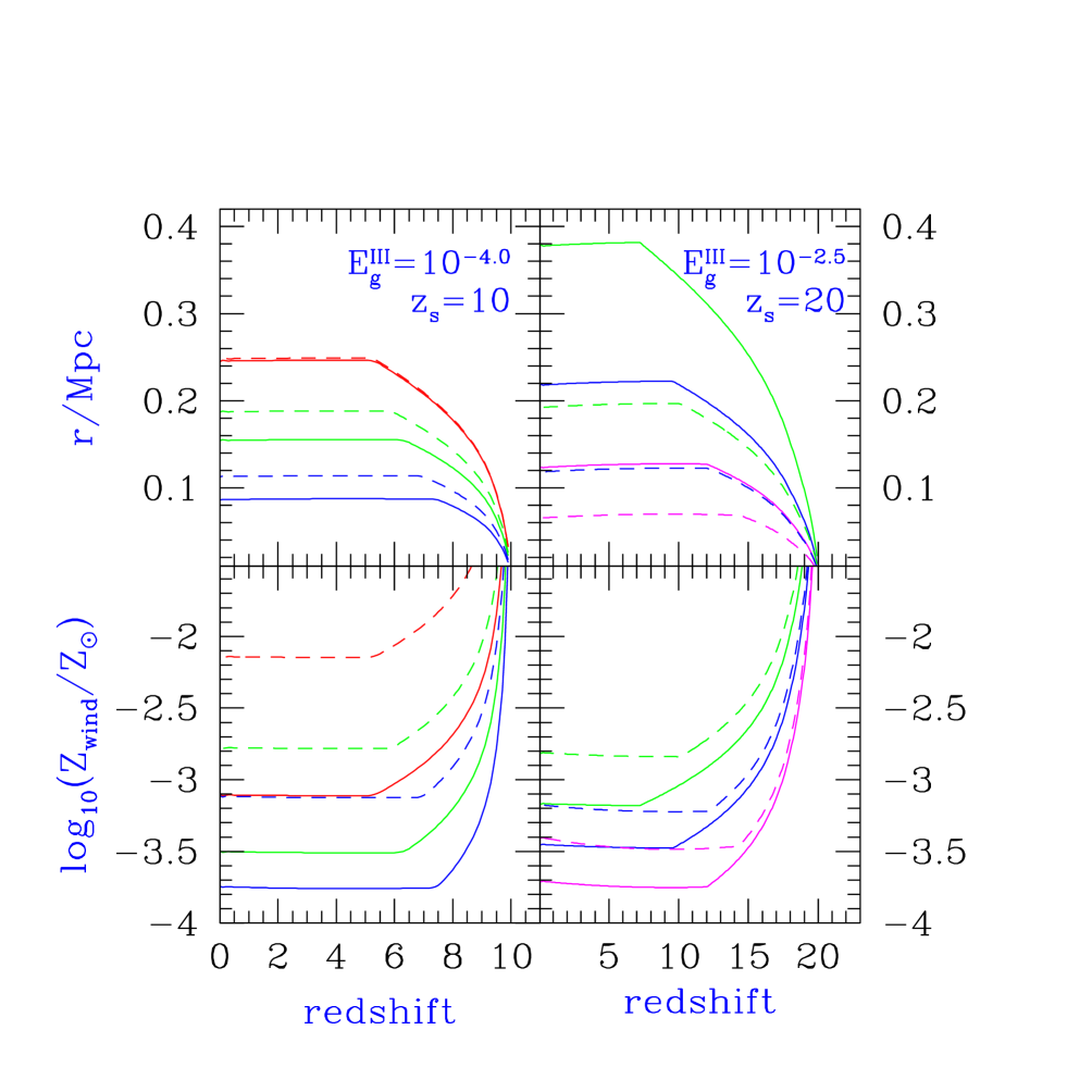
Figure 1.— Cosmological metal dispersal. Top: Comoving radii of winds emanating from PopIII (solid lines) and PopII/I (dashed) objects. In the left panel we take ${\cal E}_{\rm g}^{III}=10^{-4.0}$ and $z_{s}=10$ and consider sources at three mass scales, taken to be (from top to bottom) $10^{9}M_{\odot}$, $10^{8}M_{\odot}$, $10^{7}M_{\odot}$, corresponding to fluctuations of initial sizes 190kpc, 90kpc, and 74 kpc, respectively. In the right panel we take ${\cal E}_{\rm g}^{III}=10^{-2.5}$ and $z_{s}=20$ and consider $10^{8}M_{\odot}$, $10^{7}M_{\odot}$, and $10^{6}M_{\odot}$ objects, the smallest of which corresponds to fluctuations with a radius of 19 kpc. Bottom: Mean gas metallicity within each bubble. The lines represent the same models as in the upper panels, with $Z_{\rm wind}$ increasing as a function of source mass.

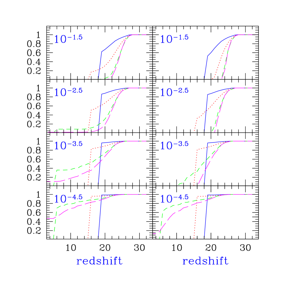
Figure 2.— Evolution of PopIII objects. Left: Fraction of PopIII objects for the best-guess models as a function of formation redshift for various masses and outflow energies. Each panel is labeled according to the energy input per gas mass, ${\cal E}_{\rm g}^{III}.$ In each panel the solid line, dotted, short dashed, long dashed lines indicate objects of masses $4.0\times 10^{6}M_{\odot}$, $1.0\times 10^{7}M_{\odot}$, $4.0\times 10^{7}M_{\odot}$, and $1.0\times 10^{8}M_{\odot}$ respectively. The sharp drop in $f_{III}$ at the smallest masses is due to the $M_{\rm min}$ cutoff. Right: Fraction of PopIII objects for the conservative models, curves are the same as in the left panels.

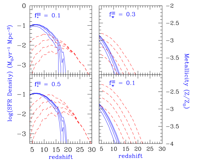
Figure 3.— Star formation rate densities for PopIII and PopII/I objects. Top Left : Star formation rate density per cubic comoving Mpc for PopIII objects (dashed lines) and PopII/I objects (solid lines). In this panel we assume $f_{\star}^{III}=f_{\star}^{II}=0.1$ and consider models in which, from top to bottom, $\log({\cal E}_{\rm g}^{III})$ = $-4.0$ $-3.5$, $-3.0$, and $-2.5$. Bottom Left : Star formation rate densities in models in which $f_{\star}^{III}=0.5$, for slightly larger $\log({\cal E}_{\rm g}^{III})$ values of $-3.5$ though $-2.0.$ Top Right: IGM average metallicity from PopIII (dashed lines) and PopII/I (solid lines) objects. Here $f_{w}=0.3$ and $\log({\cal E}_{\rm g}^{III})$ ranges from $-4.0$ to$-2.5$ from bottom to top, as increasing feedback corresponds to additional SN_γγ , which generate more metals. Bottom Right: IGM average metallicity with $f_{w}=0.1$, lines are as above.

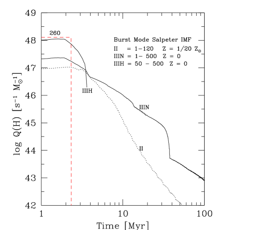
Figure 4.— Ionizing photon rate per unit stellar mass formed as a function of time in various (burst) models of star formation. The dotted line (labeled II) corresponds to PopII/I stars with metallicity of 0.05 solar and a Salpeter IMF for a range of stellar masses from $1-120{M_{\odot}}$. The solid lines correspond to PopIII stars. The extended curve (labeled IIIN) is for a Salpeter IMF for a range of stars with masses from $1-500{M_{\odot}}$, while the peaked curve (IIIH) is for a “top heavy” Salpeter IMF, with a range of stars with masses from $50-500{M_{\odot}}$. Finally, the dashed curve is the luminosity per solar mass for a single metal-free star with a mass of $260{M_{\odot}}$.

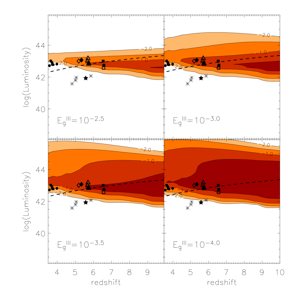
Figure 5.— Fraction of PopIII objects as a function of Ly$\alpha$ luminosity and redshift. Isocontours of fractions $\geq 10^{-2},10^{-1.5},10^{-1}$ and $10^{0.5}$ are shown. Burst-mode star formation with a $f_{\star}^{II}=f_{\star}^{III}=0.1$ is assumed for all objects, and we adopt model $II$ for $Q(H)$ in PopII/I galaxies as given in Figure 4. In the PopIII case however, we assume a lower cutoff mass of $50{M_{\odot}}$ as given by model $IIIH$, in this figure. Each panel is labeled by the assumed ${\cal E}_{\rm g}^{III}$ value. For reference, the dashed line gives the luminosity corresponding to an observed flux of $1.5\times 10^{-17}$ ergs cm^-2 s^-1, and the various points correspond to observed galaxies. The filled diamond is from Dey et al. (1998), the filled triangle is from Hu et al. (1999), the filled star is from Ellis et al. (2001), the open diamond is from Dawson et al. (2002), the open square is from Hu et al. (2002), the asterisks are from Lehnert & Bremer (2002), the open triangles are from Rhoads et al. (2002), the filled circles are from Fujita et al. (2003), and the filled squares are from Kodaira et al. (2003). Observations by Weyman (1998) and Ajiki (2002) are omitted for clarity of presentation. The curves have been extended slightly past $z=4$ for comparison with the Fujita et al. (2003) data-set.

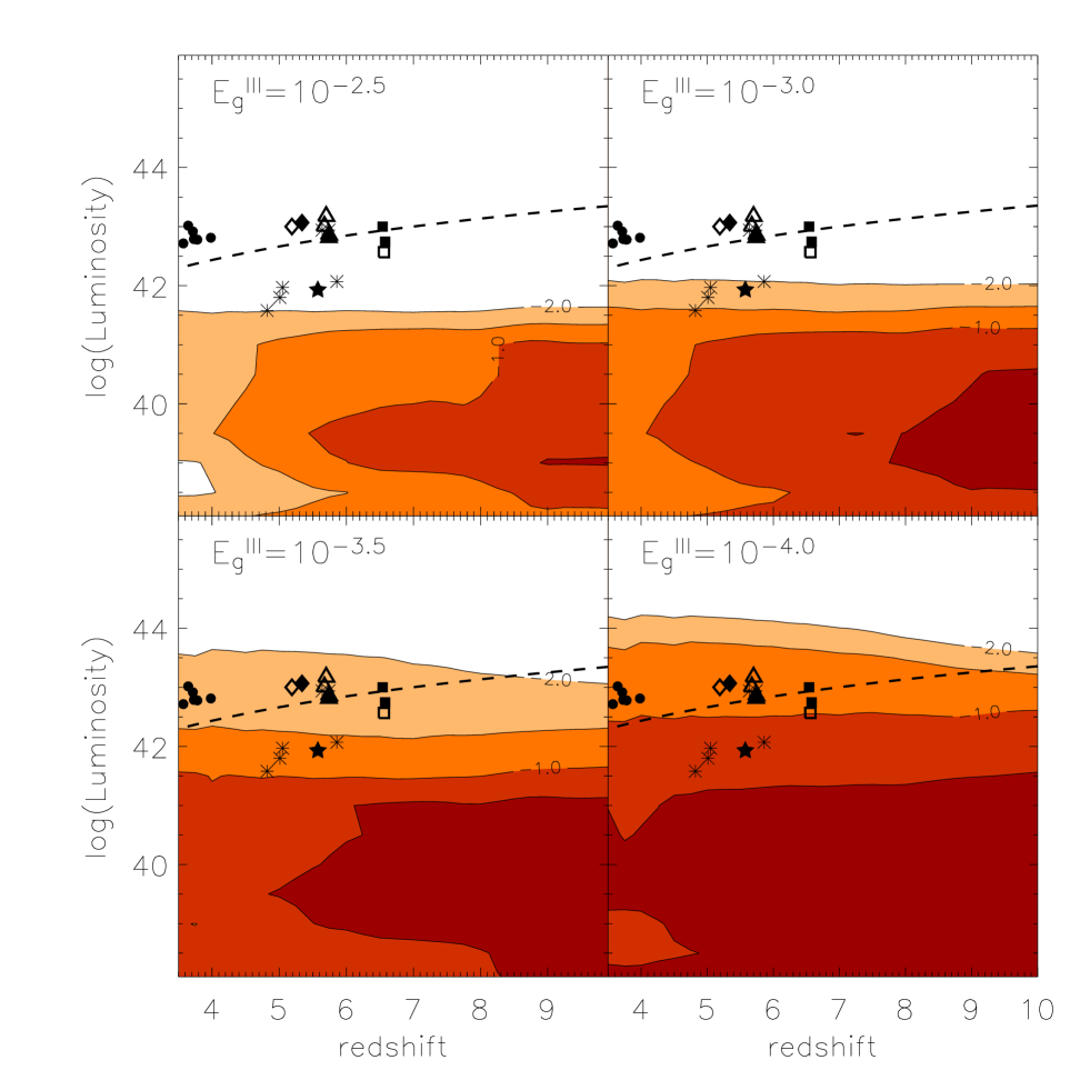
Figure 6.— Fraction of PopIII objects as a function of Ly$\alpha$ luminosity and redshift. In this case a Salpeter IMF with cutoff masses of $1-500{M_{\odot}}$ is taken for PopIII objects, greatly lowering their luminosities. The dashed lines and points are as in Figure 5.

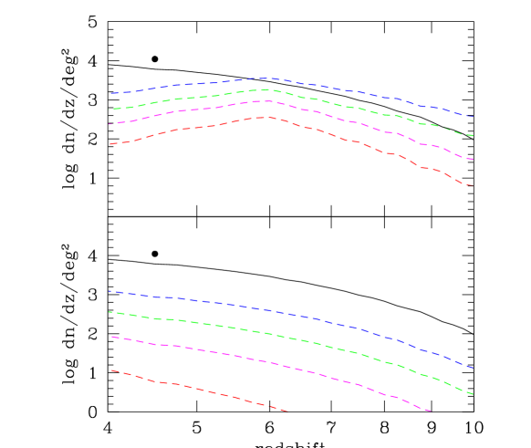
Figure 7.— Number counts of Ly$\alpha$ emitters per unit redshift and square degree as a function of redshift in various models of outflow generation. Top: Number counts assuming a top-heavy IMF as in Fig. 5. The dashed lines give the total number of Pop III emitters in models with assumed $\log_{10}({\cal E}_{\rm g}^{III})$ values (from bottom to top) of $-2.5$, $-3.0$, $-3.5$, and $-4.0$. The solid line gives the number counts of PopII/I objects in the $\log_{10}({\cal E}_{\rm g}^{III})=-3.0$ model, but is largely independent of this value. A threshold of $1.5\times 10^{-17}{\rm ergs}\,{\rm cm}^{-2}{\rm s}^{-1}$ is assumed in all cases. Bottom: Curves as in the upper panels, but assuming a Salpeter IMF as in Fig. 6. The filled circle gives the value observed by Hu et al. (1998).

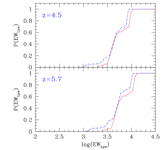
Figure 8.— Distribution of Ly$\alpha$ PopIII observed equivalent widths at two characteristic redshifts of $4.5$ (upper panel) and $5.7$ (lower panel) for a top-heavy IMF (solid), and two models assuming a $1-500{M_{\odot}}$ Salpeter IMF with $\log({\cal E}_{\rm g}^{III})=-3.5$ (dotted) and $\log({\cal E}_{\rm g}^{III})=-4.0$ (dashed). The upper panel in this figure is directly comparable to a possible PopIII contribution to the distribution in Fig 1. of Malhotra & Rhoads (2002)

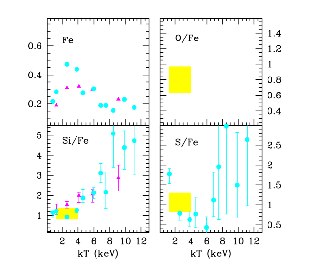
Figure 9.— Observed Fe abundance and O, Si and S abundance ratios relative to iron as a function of cluster richness. The data are normalized to solar photospheric values from Anders & Grevesse (1989). Each data point represents an average over clusters with similar richness. Triangles indicate ASCA observations and are taken from Table 2 of Fukazawa et al. (1998); dots indicate the results of a recent analysis of ASCA archival data by Baumgartner et al. (2002); the solid regions represent the average values observed by XMM (Tamura et al. 2002).

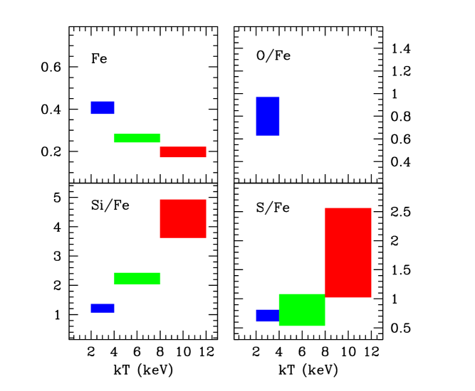
Figure 10.— Observed Fe abundance and O, Si and S abundance ratios relative to iron averaged over three cluster richness bins: [2-4] keV, [4-8] keV; [8-12] keV. The data are normalized to solar photospheric values from Anders & Grevesse (1989).

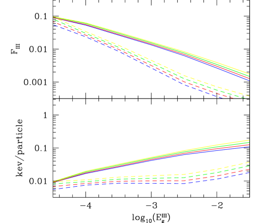
Figure 11.— Top: Fraction of cluster gas mass that has collapsed into PopIII objects as a function of energy input; solid lines correspond to the best-estimate model, and the dashed lines correspond to the conservative model. In each model the lines indicate (from top to bottom) clusters with collapse redshifts of 2, 1.5, 1, and 0.5 respectively. Even in the lowest-energy, best-estimate model at most 10% of the cluster gas is processed by PopIII objects. Bottom: An optimistic estimate of the level of ICM heating due to PopIII outflows. Here we take $f_{w}=0.1$ for all values of ${\cal E}_{\rm g}^{III}$ but assume that all of the supernova energy ${\cal E}_{\rm g}^{III}f_{w}^{-1}$, is injected into the ICM. Even in this case the energy input in all models falls far short of the observed 1 kev/particle level of preheating.

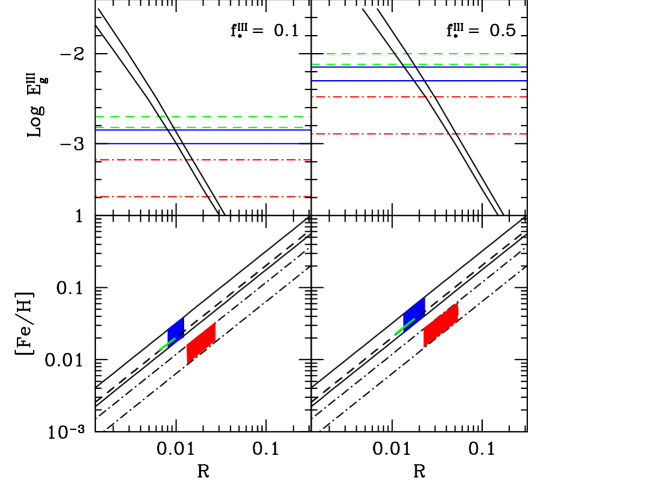
Figure 12.— Top Panels: Predicted ratio ${\cal R}=M^{III}_{\star}/M_{\star}$ as a function of the energy per unit gas mass ${\cal E}^{III}_{\rm g}$ assuming clusters formation redshifts 0.5 (lower curve) and 2 (higher curve). Horizontal lines indicate the predicted ${\cal E}^{III}_{\rm g}$ for models SN_γγ -B (dashed), SN_γγ -C (solid) and SN_γγ -D (dot-dashed) with values for $\sigma_{C}^{\rm min}$ and $\sigma_{C}^{\rm max}$ as given in Table 2 assuming two different values for the PopIII star formation efficiencies: $f^{III}_{*}=0.1$ (left panel) and $f^{III}_{*}=0.5$ (right panel). The intersection with the predicted ${\cal R}=M^{III}_{\star}/M_{\star}$ indicate the range of values for this parameter appropriate for each model. Bottom Panels: Predicted iron abundance in different SN_γγ models (with the same line coding as in top panels) as a function of ${\cal R}$. The solid regions indicate the range of Fe abundances that might be achieved in different models assuming the appropriate range of values for ${\cal R}$ (see text). Left and right panels reflects the two different star formation efficiencies.

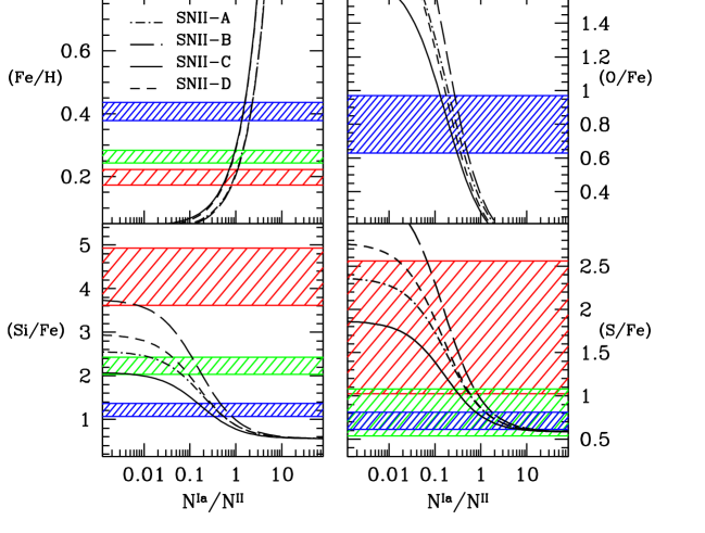
Figure 13.— Predicted ICM (Fe/H), (Si/Fe), (O/Fe) and (S/Fe) abundances (in solar values) as a function of the relative number of SNIa and SNII. Dashed regions indicate the range of observed values in three cluster richness bins as in Fig. 10 and the different lines correspond to different SNII progenitor models (see Table 1).

Figure 14.— Predicted ICM (Fe/H), (Si/Fe), (O/Fe) and (S/Fe) abundances (in solar values) as a function of the relative rate of Type Ia over Type II SNe assuming model SN_γγ -B for PopIII stars and model SNII-B for Type II SNe. The long and short-dashed lines correspond to the limiting values for ${\cal R}$ allowed by the model (see Fig. 12). For comparison, the solid line shows the predicted abundances if only Type Ia and Type II SNe contribute to the ICM enrichment. Dashed regions indicate the range of observed values in three cluster richness bins as in Fig. 10.

References

- (1)
- (2) Abel, T., Anninos, P., Norman, M. L., & Zhang, Y. 1998, ApJ, 518
- (3) Abel, T., Bryan, G., & Norman, M. 2000, ApJ, 540, 39
- (4) Ajiki, M. et al. 2002, ApJ, 576, 25
- (5) Anders, E. & Grevesse, N. 1989, Geochim. Cosmochim. Acta, 53, 197
- (6) Balbi, A. et al. 2000, ApJ, 545, L1
- (7) Barkana, R., New Astronomy, 7, 337
- (8) Beers, T. C. 2000, in The First Stars, A. Weiss et al. eds., (Berlin: Springer), 3
- (9) Bond, J. R., Cole, S., Efstathiou, G., & Kaiser, N. 1991, ApJ, 379, 440
- (10) Baumgartner, W. H., Mushotzky, R. F., Horner, D. J. 2002, in “Matter and Energy in Clusters of Galaxies”, ASP Conference Proceedings, S. Bowyer and C. Y. Hwang eds, San Francisco: Astronomical Society of the Pacific, 2002
- (11) Bialek, J. J., Evrard, A. E., & Mohr, J. J. 2001, ApJ, 555, 597
- (12) Borgani, S., Governato, F., Wadsley, J., Menci, N., Tozzi, P., Lake, G., Quinn, T. & Stadel, J. 2001, ApJ, 559, 71
- (13) Brighenti, F. & Mathews, W. G. 2001, ApJ, 553, 103
- (14) Bromm, V., Coppi, P. S., & Larson, R. B. 1999, ApJ, 527, L5
- (15) Bromm, V., Ferrara, A., Coppi, P. S., & Larson, R. B. 2001, MNRAS, 328, 969
- (16) Bromm, V., Kudritzki, R. P., & Loeb, A. 2001, ApJ, 552, 464
- (17) Bromm, V., Coppi, P.S., & Larson, R.B., 2002, ApJ, 564, 23
- (18) Cavaliere, A., Menci, N., & Tozzi, P. 1998, ApJ, 501, 493
- (19) Cavaliere, A., Menci, N., & Tozzi, P. 1999, MNRAS, 308, 559
- (20) Cayrel, R. 1996, A&AR, 7, 217
- (21) Cen, R. & Bryan, G. 2001, ApJ, 546, L81
- (22) Christlieb, N., Bessell, M. S., Beers, T. C., Gustafsson, B., Korn, A., Barklem, P. S., Karlsson, T., Mizuno-Wiedner, M. & Rossi, S. 2002, Nature, 419, 904
- (23) Ciardi, B., Ferrara, A., Governato, F., & Jenkins, A. 2000, MNRAS, 314, 611
- (24) Ciardi, B., & Ferrara, A. 2001, MNRAS, 324, 648
- (25) Ciardi, R., Bianchi, S., & Ferrara, A. 2002, MNRAS, 331, 463
- (26) Dawson, S., Spinrad, H., Stern, D., Dey, A., van Breugel, W., de Vries, W., & Reuland, M. 2002, ApJ, 570, 92
- (27) Dey, A., Spinrad, H., Stern, D., Graham, J. R., & Chaffee, F. H. 1998, ApJ 498, 93
- (28) Ellis et al. 2001, ApJL, 560, 119
- (29) Ellison, S. L., Songaila, A., Schaye, J., & Pettini, M. 2000, AJ, 120, 1175
- (30) Ferrara, A. 2001, in “The Physics of Galaxy Formation”, Tsukuba, Japan, ASP Series, eds. H. Susa, & M. Umemura, 301
- (31) Ferrara, A., Pettini, M., & Shchekinov, Y. 2000, MNRAS, 319, 539
- (32) Ferreras, I. & Silk, J. 2000, ApJ, 532, 193
- (33) Finoguenov, A., David, L. P., & Ponman, T. J. 2000, ApJ, 544, 188
- (34) Frye, B., Broadhurst, T., & Benítez, N. 2002, ApJ, 568, 558
- (35) Fukazawa, Y., Makishima. K, Tamura, T., Ezawa, H., Xu, H., Ikebe, Y., Kikuchi, K., & Ohashi, T. 1998, PASJ, 50, 187
- (36) Fujita, S. S. et al. 2003, AJ, 125, 13
- (37) Fusco-Femiano, R. & Matteucci, F. 2002, in “Chemical Enrichment of Intracluster and Intergalactic Medium”, ASP Conference Proceedings, Vol. 253, R. Fusco-Femiano and F. Matteucci eds, San Francisco: Astronomical
- (38) Furlanetto, S. & Loeb, A. ApJ, accepted, (astro-ph/0211496)
- (39) Gibson, B. K., Loewenstein, M. and Mushotzky, R. F. 1997, MNRAS, 290, 623
- (40) Gastaldello, F. & Molendi, S. 2002, ApJ, 572, 160
- (41) Gnedin, N. Y. & Ostriker J. P. 1997, ApJ, 486, 581
- (42) Haiman, Z., & Spaans, M. 1999, ApJ, 518, 138
- (43) Heger, A. & Woosley, S. E. 2002, ApJ, 567, 532
- (44) Hu, E. M. & Cowie, L. L. 1999, & McMahon 1998 ApJ, 502, L99
- (45) Hu, E. M., McMahon, R. G., & Cowie, L. L. 1999, ApJ, 522, L9
- (46) Hu, E. M., Cowie, L. L., McMahon, R. G., Capak, P., Iwamuro, F., Kneib, J.-P., Maihara, T., & Motohara, K. 2002, ApJ, 568, L75
- (47) Kaastra, J. S., Ferrigno, C., Tamura, T., Paerels, F. B. S., Peterson, J. R., & Mittaz, J. P. D. 2001, A&A, 365, L99
- (48) Kaiser, N. 1986, MNRAS, 222, 323
- (49) Kaiser, N. 1991, ApJ, 383, 104
- (50) Kodaira, K. et al. 2003, PASJ Letters, submitted (astro-ph/0301096)
- (51) Lacey, C. & Cole, S. 1993, MNRAS, 262, 627
- (52) Leitherer, L. et al. 1999, ApJS, 123, 3
- (53) Lehnert, M. D. & Bremer, M. 2002, ApJ, submitted (astro-ph/0212431)
- (54) Lloyd-Davies, E. J., Ponman, T. J., & Cannon, D. B. 2000, MNRAS, 315, 689
- (55) Loewenstein, M. 2000, ApJL, 532, 17
- (56) Loewenstein, M. 2001, ApJL, 557, 573
- (57) Mackey, J., Bromm, V., & Hernquist, L. ApJ, submitted (astro-ph/0208447)
- (58) Madau, P., Ferrara, A., & Rees, M. J. 2001, ApJ, 555, 9
- (59) Malhotra, S. & Rhoads, J. E. 2002, ApJ, 565, L71
- (60) McWilliam, A., Preston, G. W., Sneden, C., & Searle, L. 1995, AJ, 109, 2757
- (61) Mo, H. J. & White, S. D. M. 1996, MNRAS, 282, 347
- (62) Mori, M., Ferrara, A., & Madau P. 2002, ApJ, 571, 40
- (63) Nagasato, N. & Shigeyama, T. 2000, ApJ, 541, L59
- (64) Nakamura, F. & Umemura, M. 1999, ApJ, 515, 239
- (65) Nakamura, F. & Umemura, M. 2001, ApJ, 548, 19
- (66) Neufeld, D. A. 1991, ApJ 370, L85
- (67) Netterfield, C. B. et al. 2002, ApJ, 571, 604
- (68) Oh, S. P., Nollett, K. M., Madau, P., & Wasserburg, G. J. 2001, ApJ, 562, L1
- (69) Oh, S. P., Haiman, Z., & Rees, M. J. 2001, ApJ, 553, 730
- (70) Omukai, K. & Nishi, R. 1998, ApJ, 508, 141
- (71) Omukai, K. 2000, ApJ, 534, 809
- (72) Ostriker, J. P. & McKee, C. F. 1988, Rev. Mod. Phys., 60, 1
- (73) Peterson, J. R. et al. 2001, A&A, 365, L104
- (74) Pipino, A., Matteucci, F., Borgani, S., & Biviano, A. 2002, New Astronomy, 7, 227
- (75) Porciani, C., Matarrese, S., Lucchin, F., & Catelan, P. 1998, MNRAS, 298, 1097
- (76) Press, W. H., & Schechter, P. 1974, ApJ, 187, 425
- (77) Pryke, C. et al. 2002, ApJ, 568, 46
- (78) Renzini, A. 1997, ApJ, 488, 35
- (79) Renzini, A. 1999, in Chemical Evolution from Zero to High Redshift, ed. J. Walsh, & M. Rosa (Berlin: Springer), 185
- (80) Rhoads, J. E. et al. 2002, AJ, submitted, (astro-ph/0209544)
- (81) Ripamonti, E., Haardt, F., Ferrara, A., & Colpi, M. 2002, MNRAS, 334, 401
- (82) Rosati, P., Borgani, S., & Norman, C. 2002, ARA&A, 40, 539
- (83) Ryan, S. G., Norris, J. E., & Beers, T. C. 1996, ApJ, 471, 254
- (84) Salvaterra, R. & Ferrara, A. 2003, MNRAS, submitted (astro-ph/0210331)
- (85) Scannapieco, E. & Barkana, R. 2002, ApJ, 571, 585
- (86) Scannapieco, E. & Broadhurst, T. 2001, ApJ, 549, 28
- (87) Scannapieco, E., Ferrara, A., & Madau P. 2002, ApJ, 574, 590
- (88) Schaerer, D. 2002, A&A, 382, 28
- (89) Schaerer, D., & Pelló 2001, A&SS, 281, 475
- (90) Schaye, J., Rauch, M., Sargeant, W. L. W., & Kim, T. S. 2000, ApJ, 541, L1
- (91) Schneider, R., Ferrara, A., Natarajan, P., & Omukai, K. 2002, ApJ, 571, 30
- (92) Schneider, R., Guetta, D., & Ferrara, A. 2002, MNRAS, 334, 173
- (93) Schneider, R., Ferrara, A., Salvaterra, R., Omukai, K., & Bromm, V. 2003, submitted to Nature
- (94) Songaila, A. 2001, ApJ, 561, L153
- (95) Tamura, T. et al. 2001a, A & A, 365, L93
- (96) Tamura, T., Bleeker, J. A. M., Kaastra, J. S., Ferrigno, C. & Molendi, S. 2001b, A & A, 379, 107
- (97) Tamura, T., Kaastra, J. S., Bleeker, J. A. M., Ferrigno, C., Peterson, J. R., 2002, in ”New Visions of the X-ray Universe in the Xmm-Newton and Chandra Era”, ESA SP-488, F. Jansen & TBD, eds
- (98) Tegmark, M., Silk, J., & Evrard, A. 1993, ApJ, 417, 54
- (99) Thacker, R. J., Scannapieco, E., & Davis, M. 2002, ApJ, 581, 36
- (100) Tozzi, P. & Norman, C. 2001, ApJ, 546, 63
- (101) Tozzi P, Scharf C, Norman C. 2001, ApJ, 542, 106
- (102) Tsujimoto, T., Nomoto, K., Yoshii, Y., Hashimoto, M., Yanagida, S., Thielemann, F., K. 1995, MNRAS, 277, 945
- (103) Tumlinson, J., Giroux, M. & Shull, J. M. 2001, ApJ, 555, 839
- (104) Tumlinson, J., Shull, J. M., & Venkatesan A. 2002, ApJ, accepted, (astro-ph/0206389)
- (105) Umeda, H. & Nomoto, K. 2002, ApJ, 565, 385
- (106) Venkatesan, A., Tumlinson, J. & Shull, J. M. 2002, ApJ, accepted (astro-ph/0206390)
- (107) Viana, P. T. P. & Liddle, A. 1996, MNRAS, 281, 323
- (108) Voit, G. M. & Bryan, G. L. 2001, Nature, 414, 425
- (109) Weiss, A., Cassisi, S., Schlattl, H., & Salaris, M. 2000, ApJ, 553, 413
- (110) Weyman, R. J., Stern, D., Bunker, A., Spinrad, H., Chaffee, F. H., Thompson, R. I., & Storrie-Lombardi, L. J. 1998, ApJ, 505, L95
- (111) White, D. A. 2000, MNRAS, 312, 663
- (112) Woosley, S. E. & Weaver, T. A. 1995, ApJS, 101, 81
- (113) Wu, K. K. S., Fabian, A. C., & Nulsen, P. E. J. 2000, MNRAS, 318, 889