Blue Supergiants as a Tool for Extragalactic Distances – Theoretical Concepts

Abstract

Because of their enormous intrinsic brightness blue supergiants are ideal stellar objects to be studied spectroscopically as individuals in galaxies far beyond the Local Group. Quantitative spectroscopy by means of efficient multi-object spectrographs attached to 8m-class telescopes and modern NLTE model atmosphere techniques allow us to determine not only intrinsic stellar parameters such as effective temperature, surface gravity, chemical composition and absolute magnitude but also very accurately interstellar reddening and extinction. This is a significant advantage compared to classical distance indicators like Cepheids and RR Lyrae. We describe the spectroscopic diagnostics of blue supergiants and introduce two concepts to determine absolute magnitudes. The first one (Wind Momentum – Luminosity Relationship) uses the correlation between observed stellar wind momentum and luminosity, whereas the second one (Flux-weighted Gravity – Luminosity Relationship) relies only on the determination of effective temperature and surface gravity to yield an accurate estimate of absolute magnitude. We discuss the potential of these two methods.

1 Introduction

The best established stellar distance indicators, Cepheids and RR Lyrae, suffer from two major problems, extinction and metallicity dependence, both of which are difficult to determine for these objects with sufficient precision. Thus, in order to improve distance determinations in the local universe and to assess the influence of systematic errors there is definitely a need for alternative distance indicators, which are at least as accurate but are not affected by uncertainties arising from extinction or metallicity. It is our conviction that blue supergiants are ideal objects for this purpose. The big advantage is the enormous intrinsic brightness in visual light, which makes them available for accurate quantitative spectroscopic studies even far beyond the Local Group using the new generation of 8m-class telescopes and the extremely efficient multi-object spectrographs attached to them bresolin01 . Quantitative spectroscopy allows us to determine the stellar parameters and thus the intrinsic energy distribution, which can then be used to measure reddening and the extinction law. In addition, metallicity can be derived from the spectra. We emphasize that a reliable spectroscopic distance indicator will always be superior, since an enormous amount of additional information comes for free, as soon as one is able to obtain a reasonable spectrum.

In this review we concentrate on blue supergiants of spectral types late B to early A. These are the the brightest “normal” stars at visual light with absolute magnitudes $-7.0\geq M_{V}\geq-9.5$, see bres03 . By “normal” we mean stars evolving peacefully without showing signs of eruptions or explosions, which are difficult to handle theoretically and observationally.

Figure 1 shows the location of these objects in a Hertzsprung-Russell diagram (HRD) with theoretical evolutionary tracks. With initial ZAMS-masses between 15 and 40 M_⊙ they do not belong to the most massive and the most luminous stars in galaxies. O-stars can be significantly more massive and luminous, however, because of their high atmospheric temperatures they emit most of their radiation in the extreme and far UV. Late B and early A supergiants are cooler and because of Wien’s law their bolometric corrections are small so that their brightness at visual light reaches a maximum value during stellar evolution.

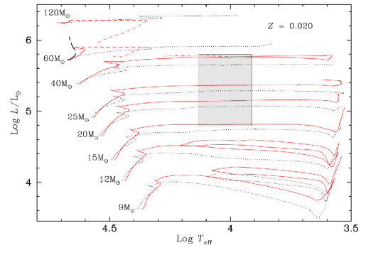
Figure 1: Evolutionary tracks of massive stars in the Hertzsprung-Russell diagram and the location of blue supergiants of late B and early A spectral types (shaded box). The tracks are from meynet00 . Solid tracks include the effects of stellar rotation, whereas dotted tracks are for non-rotating stars. Solar metallicity has been adopted for the calculations. The tracks are labelled by the initial masses (in solar units) at the zero-age main sequence (ZAMS). Note that effects of mass-loss due to stellar winds are included in the calculations so that actual masses are smaller than ZAMS-masses in later stages of the evolution

In the temperature range of late B and early A-supergiants there are also always a few objects brighter than M_V $=$ $-$9.5 . Generally, those are more exotic objects such as Luminous Blue Variables (LBVs) with higher initial masses and with spectra characterized by strong emission lines and sometimes in dramatic evolutionary phases with outbursts and eruptions. Although their potential as distance indicators is also very promising, we regard the physics of their evolution and atmospheres as too complicated at this point and, thus, exclude them from our discussion.

The objects of our interest evolve smoothly from the left to the right in the HRD crossing the temperature range of late B and early A-supergiants on the order of several $10^{3}$ years meynet00 . During this short evolutionary phase stellar winds with mass-loss rates of the order $10^{-6}$ M_⊙ yr^-1 or less kud2000 do not have time enough to reduce the mass of the star significantly so that the mass remains constant. In addition, as Fig. 1 shows, the luminosity stays constant as well. The fact that the evolution of these objects can very simply be described by constant mass, luminosity and a straightforward mass-luminosity relationship makes them a very attractive stellar distance indicator, as we will explain later in this review.

As evolved objects the blue supergiants are older than their O-star progenitors, with ages between 0.5 to 1.3 $\times$ $10^{7}$ years meynet00 . All galaxies with ongoing star formation or bursts of this age will show such a population. Because of their age they are spatially less concentrated around their place of birth than O-stars and can frequently be found as isolated field stars. This together with their intrinsic brightness makes them less vulnerable as distance indicators against the effects of crowding even at larger distances, where less luminous objects such as Cepheids and RR Lyrae start to have problems.

With regard to the crowding problem we also note that the short evolutionary time of $10^{3}$ years makes it generally very unlikely that an unresolved blend of two supergiants with very similar spectral types is observed. On the other hand, since we are dealing with spectroscopic distance indicators, any contribution of unresolved additional objects of different spectral type is detected immediately, as soon as it affects the total magnitude significantly.

Thus, it is very obvious that blue supergiants seem to be ideal to investigate the properties of young populations in galaxies. They can be used to study reddening laws and extinction, detailed chemical composition, i.e. not only abundance patterns but also gradients of abundance patterns as a function of galactocentric distance, the properties of stellar winds as function of chemical composition and the evolution of stars in different galactic environment. Most importantly, as we will demonstrate below, they are excellent distance indicators.

It is also very obvious that the use of blue supergiants as tools to understand the physics of galaxies and to determine their distances depends very strongly on the accuracy of the spectral diagnostic methods which are applied. The attractiveness of blue supergiants for extragalactic work, namely their outstanding intrinsic brightness, has also always posed a tremendous theoretical problem. The enormous energy and momentum density contained in their photospheric radiation field leads to significant departures from Local Thermodynamic Equilibrium and to stellar wind outflows driven by radiation. It has long been a problem to model non-LTE and radiation driven winds realistically, but significant theoretical progress was made during the past decade resulting in powerful spectroscopic diagnostic tools which allow to determine the properties of supergiant stars with high precision.

We describe the status quo of the spectroscopic diagnostics in the following chapters. We will then demonstrate how the spectroscopic information can be used to determine distances. We will introduce two completely independent theoretical concepts for distance determination methods. The first method, the Wind Momentum – Luminosity Relationship (WLR), uses the strengths of the radiation driven stellar winds as observed through the diagnostics of H_α as a measure of absolute luminosity and, therefore, distance. The second method, the Flux-weighted Gravity – Luminosity Relationship (FGLR), determines the stellar gravities from all the higher Balmer lines and uses gravity divided by the fourth power of effective temperature as a precise measure of absolute magnitude. A short discussion of the potential of these new concepts will conclude the paper.

2 Stellar Atmospheres and Spectral Diagnostics

The physics of the atmospheres of blue supergiant stars is complex and very different from standard stellar atmosphere models. They are dominated by the influence of the radiation field, which is characterized by energy densities larger than or of the same order as the energy density of atmospheric matter. Another important characteristic are the low gravities, which lead to extremely low densities and an extended atmospheric plasma with very low escape velocity from the star. This has two important consequences. First, severe departures from Local Thermodynamic Equilibrium (LTE) of the level populations in the entire atmosphere are induced, because radiative transitions between ionic energy levels become much more important than inelastic collisions with free electrons. Second, a supersonic hydrodynamic outflow of atmospheric matter is initiated by line absorption of photons transferring outwardly directed momentum to the atmospheric plasma. This latter mechanism is responsible for the existence of the strong stellar winds observed.

Stellar winds can affect the structure of the outer atmospheric layers substantially and change the profiles of strong optical lines such as H_α and H_β significantly. The effects of the departures from Local Thermodynamic Equilibrium (“NLTE”) can also become crucial depending on the atomic properties of the ion investigated. A comprehensive and detailed discussion of the basic physics behind these effects and the advancement of model atmosphere work for blue supergiants is given in kud88 and kud98 . More recent work is described in santolaya97 ,paul2001 and puls2002 .

For late B and early A-supergiants considerable progress has been made during the last four years in the development of a very detailed and accurate modelling of the NLTE radiative transfer enabling very precise determinations of stellar parameters and chemical abundances, see becker98 , przy00 , przy01a , przy01b , przy01c and przy02 . Figure 2 gives an impression of the effort put into the atomic models and corresponding radiative transfer of individual ions.

Figure 2: Model atoms for N i (top) and N ii (bottom) as used in the NLTE model calculations for late B and early A-supergiants; from przy01a

2.1 Effective Temperature and Gravity

Effective temperature T_eff and gravity $\log g$ are the most fundamental atmospheric parameters. They are usually determined by fitting simultaneously two sets of spectral lines, one depending mostly on T_eff and the other on $\log g$. Figure 3 indicates how this is done in principle. When fitting the ionization equilibria of elements spectral lines of two or more ionization stages have to be brought into simultaneous agreement with observations. At different locations in the ($\log g$, log T_eff)-plane this can be achieved only for different elemental abundances. Thus, along the fit curve for the ionization equilibrium in Fig. 3 the abundance of the corresponding element varies and the intersection with the fit curve for the Balmer lines leads to an automatic determination of the abundance of the element, for which the ionization equilibrium is investigated. (Note that the old technique of fitting ratios of equivalent widths of lines in different ionization stages and to regard those as being independent of abundance is less reliable, since the lines might be on different parts on the curve of growth).

Figure 3: Schematic fit diagram of temperature- and gravity-sensitive spectral lines in the ($\log g$, log T_eff)-plane. Along the dashed curve the computed spectral lines of two different ionization stages of one element agree with the observations. Typical ionization equilibria for late B-supergiants are Si ii/iii, N i/ii, O i/ii and S ii/iii, and for A-supergiants one can use Mg i/ii and N i/ii. Along the solid curve the computed profiles of the higher Balmer lines agree with the observations. The intersection determines T_eff and $\log g$

For A-supergiants the technique has been pioneered by venn95 . Most recent examples for applications are przy02 , venn99 , venn01a , venn01b . Examples are given in Figs. 4–6.

The accuracy in the determination of T_eff and $\log g$, which can be achieved when using spectra of high S/N and sufficient resolution is astonishing.$\Delta$T_eff/T_eff $\sim$ 0.01 and $\Delta\log g$ $\sim$ 0.05 are realistic values.

Figure 4: Fit diagram for the supergiants $\beta$ Ori (top) and $\eta$ Leo (bottom). The curves are parameterized by surface helium abundance $y$ (by number); from przy02

Figure 5: Temperature and gravity dependence of Mg i (top) and Mg ii (bottom) of $\eta$ Leo. Results from the NLTE computations for the final stellar parameters (full line) are compared with synthetic spectra for modified parameters (dotted lines), as indicated, against observation (dots); from przy02

Figure 6: Temperature and gravity dependence of H_γ of $\eta$ Leo. See Fig. 5 for further annotations; from przy02

2.2 Chemical Composition

The development of very detailed model atoms and using new and very accurate atomic data, ip , op , has led to an enormous improvement of the precision to which elemental abundances even in extreme blue supergiants can be determined przy00 , przy01a , przy01b , przy01c , przy02 , venn01a , venn01b . On the average, the uncertainties are now reduced to 0.1 dex in the abundance relative to hydrogen. Figure 7 displays a nice example for the fit of the equivalent widths of CNO lines in blue supergiants.

The amount of information about chemical elements is impressive. Figure 8 gives an overview about the chemical elements the abundances of which can be determined from the optical spectra of blue supergiants. Figure 8 shows characteristic abundance patterns, as they can be derived for supergiants in the Milky Way and Fig. 9 displays results for two M 31 supergiants.

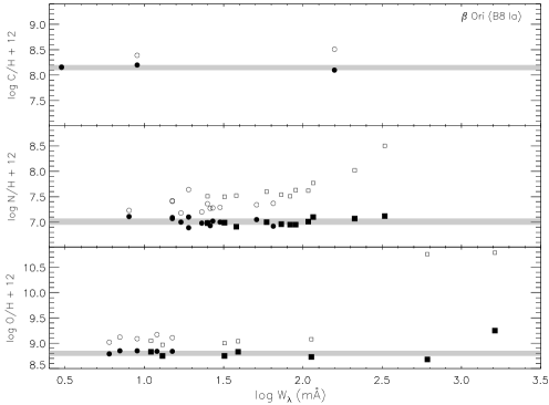
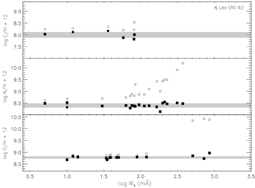
Figure 7: Element abundances derived from individual spectral lines of CNO plotted as a function of equivalent width. Top: $\beta$ Ori, bottom: $\eta$ Leo. Open symbols refer to LTE calculations for the line formation, whereas solid symbols show the results of NLTE radiative transfer, for neutral (boxes) and ionized species (circles). It is evident that LTE fails badly, in particular, for stronger lines. The NLTE results are remarkably consistent; from przy03

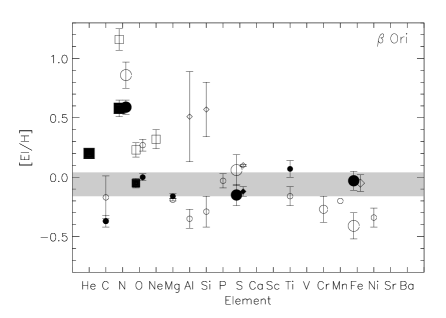
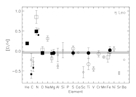
Figure 8: Abundance pattern determined for the two Milky Way supergiants $\beta$ Ori and $\eta$ Leo, relative to the solar standard grev98 on a logarithmic scale. NLTE (filled symbols) and LTE abundances (open symbols) for neutral (boxes), single-ionized (circles) and double-ionized (diamonds) species. The symbol size codes the number of spectral lines analyzed. Error bars represent 1$\sigma$-uncertainties from the line-to-line scatter. The grey shaded area marks the deduced stellar metallicity within 1$\sigma$-errors. The NLTE computations reveal a striking similarity to the solar abundance distribution, except for the light elements which have been affected by mixing with nuclear-processed matter; from przy02

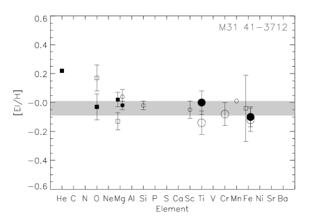
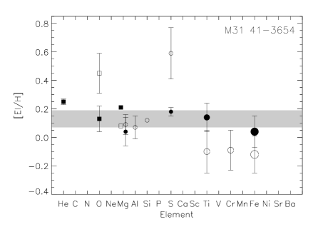
Figure 9: Abundance pattern of the two M 31 A-supergiants 41-3712 and 41-3654. See Fig. 8 for further annotations; from przy02

2.3 Stellar Wind Properties

In principle, two types of lines are formed in a stellar wind, P-Cygni profiles with a blue absorption trough and a red emission peak and pure emission profiles. The difference is caused by the re-emission process after the photon has been absorbed within the line transition. If the photon is immediately re-emitted by spontaneous emission, then we have the case of line scattering with a source function proportional to the geometrical dilution of the radiation field and a P-Cygni profile will result. If the re-emission occurs as a result of a different atomic process, for instance after a recombination of an electron into the upper level or after a spontaneous decay of a higher level into the upper level or after a collision, then the line source function will possibly not dilute and may roughly stay constant as a function of radius so that an emission line results. Typical examples for P-Cygni profiles are UV resonance transitions connected with the ground level, whereas excited lines of an ionization stage into which frequent recombination from higher ionization stages occurs will produce emission lines. H_α in O-stars and early B-supergiants is a typical example for the latter case. However, for late B- and A-supergiants, when Ly_α becomes severely optically thick and the corresponding transition is in detailed balance, the first excited level of hydrogen becomes the effective groundstate and H_α starts to behave like a resonance line showing also the shape of a P-Cygni profile (for a more comprehensive discussion of the line formation process in winds see kud88 , kud98 and the most recent review kud2000 ).

Terminal velocities can be determined very precisely from the blue edges of P-Cygni profiles and the red emission wings, normally with an accuracy of 5 to 10 percent (but see kud2000 for details). In addition, H_α profiles normally allow for a very accurate (20 percent) determination of mass-loss rates in all cases of O, B, and A-supergiants puls96 , kud99 , mccarthy97 , but see kud2000 and puls2002 for details and problems.

Figure 10 gives an impression about the accuracy of the stellar wind spectral diagnostics for A-supergiants.

Figure 10: Top: The influence of the mass-loss rate $\dot{M}$ on the H_α profile of the M 31 A-supergiant 41-3654. Two models with $\dot{M}=1.65$ and $2.15\times 10^{-6}$ M_⊙ yr^-1 (dashed-dotted, dashed) and otherwise identical parameters are shown superimposed on the observed profile. Bottom: The determination of $v_{\infty}$. Two models with $v_{\infty}=200$ and $250\,$km s^-1 (dashed, dashed-dotted) and $\dot{M}$ adopted to fit the height of the emission peak are shown superimposed to the observed profile. All other parameters are identical; from mccarthy97

2.4 Spectral Resolution

For extragalactic applications beyond the Local Group spectral resolution becomes an issue. The important points are the following. Unlike the case of late type stars, crowding and blending of lines is not a severe problem for hot massive stars, as long as we restrict our investigation to the visual part of the spectrum. In addition, it is important to realize that massive stars have angular momentum, which leads to usually high rotational velocities. Even for A-supergiants, which have already expanded their radius considerably during their evolution and, thus, have slowed down their rotation, the observed projected rotational velocities are still on the order of 30 km s^-1 or higher. This means that the intrinsic full half-widths of metal lines are on the order of 1 Å. In consequence, for the detailed studies of supergiants in the Local Group a resolution of 25,000 sampling a line with five data points is ideal. This is indeed the resolution, which has been applied in most of the work referred to in the previous sections.

However, as we have found out empirically przy02 , degrading the resolution to 5,000 (FWHM = 1 Å) has only a small effect on the accuracy of the diagnostics, as long as the S/N remains high (i.e. 50 or better). Even for a resolution of 2,500 (FWHM = 2 Å) it is still possible to determine T_eff to an accuracy of 2 percent, $\log g$ to 0.05 dex and individual element abundances to 0.1 or 0.2 dex.

References bresolin01 , bresolin02 , bresolinWN , bres03 and kud2003 have used FORS at the VLT with a resolution of 1,000 (FWHM = 5 Å) to study blue supergiants far beyond the Local Group. The accuracy in the determination of stellar properties at this rather low resolution is still remarkable. The effective temperature is accurate to roughly 4 percent and the determination of gravity remains unaffected and is still good to 0.05 dex (an explanation will be given in Sect. 4). However, at this resolution it becomes difficult to determine abundance patterns of individual elements (except for emission line stars, see bresolinWN ) and, thus, one is restricted to the determination of the overall metallicity which is still accurate to 0.2 dex.

We can conclude that an optimum for extragalactic work is a resolution of 2,500 (FWHM = 2 Å). Blue supergiants are bright enough even far beyond the Local Group to allow the achievement of high S/N with reasonable exposure times at 8m-class telescopes with efficient multi-object spectrographs at this resolution, which then makes it possible to determine stellar parameters and chemical composition with sufficient precision. This resolution is also good enough to determine stellar wind parameters from the observed H_α profiles, since the stellar wind velocities (and therefore the corresponding line widths) are larger than 150 km s^-1.

3 The Wind Momentum–Luminosity Relationship

The concept of the Wind Momentum–Luminosity Relationship (WLR) has been introduced by kud95 and puls96 . It starts from a very simple idea. The winds of blue supergiants are initiated and maintained by the absorption of photospheric radiation and the photon momentum connected to it. Thus, the mechanical momentum flow of a stellar wind $\dot{M}v_{\infty}$ should be a function of the photon momentum rate $L/c$ provided by the stellar photosphere and interior

$$\dot{M}v_{\infty}=f(L/c)\;.$$ (1)

If this is true and if we are able to find this function $f$, this would enable us to determine directly stellar luminosities from the stellar wind by using the inverse relation

$$L=f^{-1}(\dot{M}v_{\infty})\;.$$ (2)

In other words, by measuring the rate of mass-loss and the terminal velocity directly from the spectrum we would be able to determine the luminosity of a blue supergiant. This is an exciting perspective, because it would give us a completely new, purely spectroscopic tool to determine stellar distances. Quantitative spectroscopy would yield $T_{\mathrm{eff}}$, gravity, abundances, intrinsic colours, reddening, extinction, $\dot{M}$ and $v_{\infty}$. With the luminosity from the above relation one could then compare with the dereddened apparent magnitude to derive a distance.

In the previous section, we already demonstrated how $\dot{M}$ and $v_{\infty}$ can be determined from the spectrum with high precision. Thus, deriving the theoretical relationship and confirming and calibrating it observationally will enable us to introduce a new distance determination method. An accurate analytical solution of the hydrodynamic equations of line driven winds has been provided by kud89 . These solutions were then used by kud95 and puls96 to exactly derive the relationship. Here, we apply a simplified approach, see also kud98 , which is not exact but gives insight in the underlying physics.

Figure 11: Sketch of a blue supergiant irradiating its own stellar wind envelope. $L_{\nu}$ is the spectral luminosity at frequency $\nu$. $v$ is the wind outflow velocity at radius $r$ and $\varrho$ is the mass density

We assume that the wind is stationary and spherical symmetric and obeys the equation of continuity

$$\dot{M}=4\pi r^{2}\varrho(r)v(r)\;.$$ (3)

Then we consider the star as a point source of photons irradiating and accelerating its own stellar wind (see Fig. 11) and calculate the amount of photon momentum absorbed by one spectral line

$$\frac{{\hbox{$L$}}}{{\hbox{$c$}}}\frac{{\hbox{$L_{\nu_{i}}(1-e^{-\tau_{i}})\mathrm{d}\nu^{\mathrm{width}}$}}}{{\hbox{$L$}}}=\frac{{\hbox{$L$}}}{{\hbox{$c^{2}$}}}\frac{{\hbox{$\nu_{i}L_{\nu_{i}}$}}}{{\hbox{$L$}}}(1-e^{-\tau_{i}})\mathrm{d}v\;.$$ (4)

The first factor on the left side gives the total photon momentum rate provided by the star, the second describes the fraction absorbed by one spectral line in an outer shell of thickness $\mathrm{d}r$. $\tau_{i}$ is the optical thickness of such an outer shell in the line transition $i$. $L_{\nu_{i}}\mathrm{d}\nu^{\mathrm{width}}$ is the stellar spectral luminosity at the frequency of line $i$ multiplied by the spectral width of the line. This luminosity can in principle be absorbed by the line if it is entirely optically thick (i.e. $\tau_{i}\gg 1$). However, depending on the optical thickness only the fraction $(1-e^{-\tau_{i}})$ is really absorbed. If we are in the supersonic part of the wind, then the spectral width $\mathrm{d}\nu^{\mathrm{width}}$ is not determined by the thermal motion of the ions but rather by the increment of the velocity outflow $\mathrm{d}v$ via the Doppler formula

$$\mathrm{d}\nu^{\mathrm{width}}=\nu_{i}\frac{{\hbox{$\mathrm{d}v$}}}{{\hbox{$c$}}}\;,$$ (5)

which leads to the right hand side of (4).

After calculation of the photon momentum absorbed by a single spectral line we can consider the momentum balance in the stellar wind. The photon momentum absorbed by all lines will just be a sum over all lines $i$ of the expression shown on the right hand side of (4). Almost all of this absorbed momentum will be transformed into gain of mechanical stellar wind flow momentum $\dot{M}\mathrm{d}v$ of the outer shell except the fraction $g(r)\mathrm{d}M_{r}$, which is the momentum required to act against the gravitational force ($g(r)=GM_{\ast}/r^{2}$ is the local gravitational acceleration and $\mathrm{d}M_{r}=\varrho 4\pi r^{2}\mathrm{d}r$ is the mass within the spherical stellar wind shell)

$$\dot{M}\mathrm{d}v=\frac{{\hbox{$L$}}}{{\hbox{$c^{2}$}}}\sum_{i}\frac{{\hbox{$\nu_{i}L_{\nu_{i}}$}}}{{\hbox{$L$}}}(1-e^{-\tau_{i}})dv-G\frac{{\hbox{$M{\ast}(1-\Gamma)$}}}{{\hbox{$r^{2}$}}}\varrho 4\pi r^{2}\mathrm{d}r\;.$$ (6)

Note that this momentum balance also includes the photon momentum transfer by Thomson scattering, which leads to the correction factor $(1-\Gamma)$ in the local gravitational acceleration.

Now, the important next step is to deal with the sum over all lines in the above momentum balance. Here, the complication arises from the term in parentheses containing the local optical depth $\tau_{i}$ of each line. $\tau_{i}$ will not only be different for each of the thousands of lines driving the wind, it will also vary through the stellar wind as a function of radius. On the other hand, one of the enormous simplifications in supersonically expanding envelopes around stars is that the optical thickness is well described by (see for instance kud88 )

$$\tau_{i}=k_{i}\kappa_{\mathrm{Thom}}\frac{{\hbox{$v_{\mathrm{therm}}$}}}{{\hbox{$\mathrm{d}v/\mathrm{d}r$}}}\;,$$ (7)

where $v_{\mathrm{therm}}$ is the thermal velocity of the ion and $k_{i}$ is the (dimensionless) line strength defined as

$$k_{i}=\frac{{\hbox{$\kappa_{i}$}}}{{\hbox{$\kappa_{\mathrm{Thom}}$}}}\;,$$ (8)

i.e. the opacity of line $i$

$$\kappa_{i}=\frac{{\hbox{$1$}}}{{\hbox{$\Delta\nu_{\mathrm{Dopp}}$}}}\frac{{\hbox{$\pi e^{2}$}}}{{\hbox{$m_{\mathrm{e}}c$}}}n_{l}f_{lu}\left(1-\frac{{\hbox{$n_{u}$}}}{{\hbox{$n_{l}$}}}\frac{{\hbox{$g_{l}$}}}{{\hbox{$g_{u}$}}}\right)$$ (9)

in units of the continuous Thomson scattering opacity or in units of the local density

$$\kappa_{\mathrm{Thom}}=n_{\mathrm{e}}\sigma_{\mathrm{e}}=\varrho s_{\mathrm{e}}\;.$$ (10)

$\sigma_{\mathrm{e}}$ is the cross section for Thomson scattering of photons on free electrons, $n_{\mathrm{e}}$ the local number density of free electrons. In a hot plasma with hydrogen as the main constituent mostly ionized and with $Y_{\mathrm{He}}=n_{\mathrm{He}}/n_{\mathrm{H}}$ and $I_{\mathrm{He}}$ the number of electrons provided per helium nucleus we have ($m_{\mathrm{H}}$ is the mass of the hydrogen atom)

$$s_{\mathrm{e}}=\frac{{\hbox{$1+I_{\mathrm{He}}Y_{\mathrm{He}}$}}}{{\hbox{$1+4Y_{\mathrm{He}}$}}}\frac{{\hbox{$\sigma_{\mathrm{e}}$}}}{{\hbox{$m_{\mathrm{H}}$}}}\;.$$ (11)

Thus, if the degree of ionization of helium is roughly constant as a function of radius $r$ in the wind, $s_{\mathrm{e}}$ is also constant and we have

$$\tau_{i}=k_{i}s_{\mathrm{e}}\varrho(r)\frac{{\hbox{$v_{\mathrm{therm}}$}}}{{\hbox{$\mathrm{d}v/\mathrm{d}r$}}}\;,$$ (12)

with the line strength $k_{i}$ proportional to oscillator strength $f_{lu}$, wavelength $\lambda_{i}$ and the occupation number $n_{l}$ of the lower level divided by the mass density $\varrho$

$$k_{i}\propto\frac{{\hbox{$n_{l}$}}}{{\hbox{$\varrho$}}}f_{lu}\lambda_{i}\;.$$ (13)

Thus, the line strength is roughly independent of the depth in the atmosphere and is determined by atomic physics ( $f_{lu}$, $\lambda_{i}$) and atmospheric thermodynamics ($n_{l}/\varrho$). Since $\varrho$ and $\mathrm{d}v/\mathrm{d}r$ vary strongly through the wind a line can be optically thick in deeper layers

$$\tau_{i}\gg 1\Longrightarrow(1-e^{-\tau_{i}})\mathrm{d}v\approx\mathrm{d}v$$ (14)

and can become optically thin further out

$$\tau_{i}\ll 1\Longrightarrow(1-e^{-\tau_{i}})\mathrm{d}v\approx k_{i}\varrho\mathrm{d}r\;.$$ (15)

For the calculation of the photon momentum transfer this means that line contributions can have an entirely different functional form depending on the optical thickness of the lines.

This problem can be solved in a very elegant way by introducing a line strength distribution function

$$n(k,\nu)\mathrm{d}\nu\mathrm{d}k = \nu_{i} \nu \nu + \mathrm{d}\nu$$ number of lines with from (,   )

$$\mbox{and with $k$ from ($k$,\,$k$\,$+$\,$\mathrm{d}k$)}\;.$$

Since the modern hydrodynamic model atmosphere codes (see Sect. 2) contain atomic data and occupation numbers for millions of lines in NLTE, we can investigate the physics of the line strength distribution function. As it turns out, spring97 , kud2000 , puls2000 and kud02 , the distribution in line strengths – to a very good approximation – obeys a power law

$$n(k,\nu)\mathrm{d}\nu\mathrm{d}k=g(\nu)\mathrm{d}\nu k^{{\bf\alpha}-2}\mathrm{d}k\;,1\leq k\leq\infty$$ (16)

independent (to first order) of the frequency. The exponent $\alpha$ depends weakly on T_eff and varies (in the temperature range of OB-stars) between

$$\alpha=0.6\ldots 0.7\;.$$ (17)

$\alpha$ is mostly determined by the atomic physics and basically reflects the distribution function of the oscillator strengths. One can, for instance, show that for the hydrogen atom the distribution of the Lyman-series oscillator strengths is a power law with exponent $\alpha=2/3$, see kud98 . It is important to realize that $\alpha$ is not a free parameter but, instead, is well determined from the thousands of lines taken into account in the model atmosphere calculations. Examples for the power law dependence of line strengths are given in kud98 or puls2000 .

With the line strength distribution function we can replace the sum in the momentum balance by a double integral, which is then analytically solved (see also kud88 ):

$$\sum_{i}\frac{{\hbox{$\nu_{i}L_{\nu_{i}}$}}}{{\hbox{$L$}}}(1-e^{-\tau_{i}})\longrightarrow\int\limits_{0}^{\infty}\int\limits_{0}^{\infty}(1-e^{\tau(k)})\frac{{\hbox{$\nu L_{\nu}$}}}{{\hbox{$L$}}}n(k,\nu)\mathrm{d}\nu\mathrm{d}k\longrightarrow N_{o}\left\{\frac{\mathrm{d}v/\mathrm{d}r}{\varrho}\right\}^{\alpha-1}\;.$$ (18)

This means that the momentum transfer from photons to the stellar wind plasma depends non-linearly on the gradient of the velocity field. The degree of the non-linearity is determined by the steepness of the line strength distribution function $\alpha$. $N_{o}$ is proportional to the number of lines in the line strength interval $1\leq k\leq\infty$.

We can now re-formulate the momentum balance to obtain

$$\dot{M}\mathrm{d}v=\frac{{\hbox{$L$}}}{{\hbox{$c^{2}$}}}N_{o}\left\{\frac{\mathrm{d}v/\mathrm{d}r}{\varrho}\right\}^{\alpha-1}\mathrm{d}v-G\frac{{\hbox{$M_{\ast}(1-\Gamma)$}}}{{\hbox{$r^{2}$}}}4\pi r^{2}\varrho\mathrm{d}r$$ (19)

yielding a non-linear differential equation for the stellar wind velocity (note that we replaced the density through the mass conservation equation)

$$r^{2}v\frac{{\hbox{$\mathrm{d}v$}}}{{\hbox{$\mathrm{d}r$}}}=\frac{{\hbox{$L$}}}{{\hbox{$\dot{M}^{{\bf\alpha}}$}}}\frac{{\hbox{$N_{o}$}}}{{\hbox{$c^{2}$}}}(4\pi)^{\alpha-1}\left\{r^{2}v\frac{{\hbox{$\mathrm{d}v$}}}{{\hbox{$\mathrm{d}r$}}}\right\}^{\alpha}-GM_{\ast}(1-\Gamma)$$ (20)

which looks much more complicated than it really is. The solution is easy, see kud89 . We obtain $\dot{M}$ as the uniquely determined eigenvalue of the problem

$$\dot{M}\propto L^{1/\alpha}\{M_{\ast}(1-\Gamma)\}^{1-1/\alpha}$$ (21)

and a terminal velocity proportional to the escape velocity $v_{\mathrm{esc}}$

$$v_{\infty}\propto v_{\mathrm{esc}}\propto\left\{GM_{\ast}(1-\Gamma)/R_{\ast}\right\}^{1/2}\;.$$ (22)

Combining the two yields the stellar wind momentum

$$\dot{M}v_{\infty}\propto\frac{{\hbox{$1$}}}{{\hbox{$R_{\ast}^{1/2}$}}}L^{1/\alpha}\{M_{\ast}(1-\Gamma)\}^{3/2-1/\alpha}\;,$$ (23)

which – as expected – depends strongly on the luminosity but also on the photospheric radius and the expression in the parentheses, which contains the stellar mass and distance from the Eddington limit. It is this expression which can vary significantly for different blue supergiants and, therefore, causes the large scatter in the observed correlations of mass-loss rates with luminosity and terminal velocity with escape velocity as discussed previously. However, for the product of mass-loss rate and terminal velocity, the stellar wind momentum rate, the exponent of the term in brackets should be – thanks to the laws of atomic physics – very close to zero, since $\alpha\approx 2/3$. This means that to first order the wind momentum rate should be determined by

$${\bf\dot{M}v_{\infty}\propto\frac{{\hbox{$1$}}}{{\hbox{$R_{\ast}^{1/2}$}}}{\bf L}^{\bf 1/\alpha}}\;.$$ (24)

Figure 12: The Wind Momentum – Luminosity Relationship of A-supergiants. Top: observed stellar wind momentum as a function of absolute magnitude for objects in the Milky Way and M 31; from bresolin01 . Bottom: Theoretical calculations using the stellar wind code by kud02 , for solar metallicity (solid circles), 0.4 solar (open squares) and 0.1 solar (open circles)

This is the Wind Momentum - Luminosity Relationship. It predicts a strong dependence of wind momentum rate on the stellar luminosity with an exponent determined by the statistics of the strengths of the tens of thousands of lines driving the wind. It also contains a weak dependence on stellar radius which comes from the fact that the stellar wind has to work against the gravitational potential when accelerated by photospheric photons.

References puls96 , kud99 and kud2000 were the first to prove that the theoretically predicted WLR is really observed. O-stars, B and A-supergiants all follow this relationship. As to be expected, the relationship depends on spectral types, since lines of different ionization stages contribute to the mechanism of line driving at different spectra types. F. Bresolin, in this volume bres03 , gives a detailed overview about the most recent observational work on the WLR. Here, we only want to show the recent best calibration for A-supergiants using (only) four Milky Way and two M31 objects in Fig. 12. Although a calibration based on merely six objects is only moderately convincing, we are again encouraged by the small scatter over the remarkable range in luminosity. Future calibration work will be crucial to establish the method as an accurate distance indicator.

Also shown in Fig. 12 are recent theoretical stellar wind calculations for A-supergiants (R.P. Kudritzki, in prep.), which are based on the new radiation driven wind algorithm developed by kud02 . The calculations provide a clear prediction about the metallicity dependence of A-supergiant wind momenta in agreement with previous work discussed in kud2000 and the recent work by vink00 and vink2001 . F. Bresolin, in this volume bres03 , will discuss most recent extragalactic stellar wind diagnostics on blue supergiants and compare them with the model predictions.

4 The Flux-Weighted Gravity–Luminosity Relationship

It is an old idea that the strengths of the hydrogen Balmer lines and the absolute luminosities of massive stars must be related (see bres03 in this volume for an overview). The concept behind this idea is very simple. Because of the effects of Stark broadening the Balmer lines in hot stars are very sensitive to the number densities of electrons and protons in those atmospheric layers, where the wings of the Balmer lines are formed. The number densities, on the other hand, depend on the photospheric gravity as the result of the hydrostatic equilibrium in stellar photospheres. Stellar gravities, however, reflect the evolution of massive stars away from the ZAMS (where all gravities are roughly the same) towards lower effective temperatures. They become smaller, as further the star evolves, and, if we compare objects with exactly the same effective temperature, more massive supergiant stars with higher luminosities are expected to have lower gravities than their counterparts with lower mass.

We illustrate the situation by using the stellar evolution models from Fig. 1. We select three values of $T_{\mathrm{eff}}$ $=$ 12000, 9500 and 8350 K, corresponding to spectral types B8, A0 and A4, respectively (see bres03 , this volume), and calculate absolute visual magnitudes and gravities for each track at each of the three $T_{\mathrm{eff}}$ values. Figure 13 displays the corresponding correlation of $M_{V}$ with $\log g$ for each temperature. While the correlations are nicely parallel, the temperature dependence as a result of stellar evolution and bolometric correction is obvious.

Figure 13: Three steps to calculate the theoretical correlation between absolute magnitude $M_{V}$ and H_γ equivalent width $EW$ for three different values of $T_{\mathrm{eff}}$ $=$ 8350 K (crosses), 9500 K (squares), 12000 K (circles). Top: $M_{V}$ vs. $EW$. Middle: $EW$ vs. $\log g$ as obtained from model atmospheres. Bottom: $M_{V}$ vs. $\log g$ as obtained from stellar evolution

We can now calculate atmospheric models for each pair of $T_{\mathrm{eff}}$ and $\log g$ and plot calculated H_γ equivalent widths $EW$ as function of gravity and then, finally, produce a diagram of absolute magnitude versus H_γ equivalent width. This is also done in Fig. 13. Since the strengths of the Balmer lines do not only depend on gravity but also on temperature, the final correlation

$$M_{V}=f(EW(\mbox{H$\gamma$})\;,\bf{T_{eff}})$$ (25)

depends very strongly on $T_{\mathrm{eff}}$. The equivalent widths are much stronger at lower $T_{\mathrm{eff}}$ and, as an additional complication, the slope of the correlation is strongly temperature dependent. While this result is, at least qualitatively, confirmed by observation bres03 , it is clear that simple empirical magnitude – equivalent width relations will have to suffer quite some intrinsic scatter unless it is restricted to accurate spectral sub-types. We, therefore, suggest a method, which overcomes the problem of the strong temperature dependence.

Before we do this important step, we draw attention to an important detail in Fig. 13. The plot equivalent width versus $\log g$ reveals that gravities can be determined with high precision for each effective temperature. An error of $\sim$10 percent in $EW$ transforms to an error of 0.05 dex in $\log g$. Knowing that we will have many higher Balmer lines in the blue spectra of supergiants we feel confident that we can determine gravities with such accuracies, even if the spectroscopic resolution is only moderate.

We now turn to the derivation of the Flux-Weighted Gravity – Luminosity Relationship (FGLR), which was introduced very recently by kud2003 . When discussing Fig. 1 in Sect. 1 we noted that massive stars evolve through the domain of blue supergiants with constant luminosity and constant mass. This has a very simple, but very important consequence for the relationship of gravity and effective temperature along each evolutionary track. From

$$L\propto R^{2}T^{4}_{\mathrm{eff}}=\mathrm{const.};M=\mathrm{const.}$$ (26)

follows immediately that

$$M\propto g\;R^{2}\propto L\;(g/T^{4}_{\mathrm{eff}})=\mathrm{const.}$$ (27)

This means that each object of a certain initial mass on the ZAMS has its specific value of the “flux-weighted gravity” g/T${}^{4}_{\mathrm{eff}}$ during the blue supergiant stage. This value is determined by the relationship between stellar mass and luminosity, which to a good approximation is a power law

$$L\propto M^{x}\;.$$ (28)

Inspection of evolutionary calculations with mass-loss, cf. meynet94 and meynet00 , shows that $x=3$ is a good value in the range of luminosities considered, although $x$ changes towards higher masses. With the mass – luminosity power law we then obtain

$$L^{1-x}\propto(g/T^{4}_{\mathrm{eff}})^{x}\;,$$ (29)

or with the definition of bolometric magnitude $M_{\mathrm{bol}}$ $\propto$ $-2.5\log L$

$$-M_{\mathrm{bol}}=a\log(g/T_{\!\mbox{\scriptsize eff}}^{4})+b\;.$$ (30)

This is the FGLR of blue supergiants. Note that the proportionality constant $a$ is given by the exponent of the mass – luminosity power law through

$$a=2.5x/(1-x)\;.$$ (31)

and $a=-3.75$ for $x=3$. Mass-loss will depend on metallicity and therefore affect the mass – luminosity relation. In addition, stellar rotation through enhanced turbulent mixing might be important for this relation. In order to investigate these effects we have used the models of meynet94 and meynet00 to construct the stellar evolution FGLR, which is displayed in Fig. 14. The result is very encouraging. All different models with or without rotation and with significantly different metallicity form a well defined very narrow FGLR.

Figure 14: The FGLR of stellar evolution models from meynet94 and meynet00 . Circles correspond to models with rotation, squares represent models without the effects of rotation. Solid symbols refer to galactic metallicity and open symbols represent SMC metallicity. The solid curve corresponds to $a=-3.75$ in the FGLR

Figure 15: Fit of the higher Balmer lines of an A-supergiant in the Sculptor galaxy NGC 300 using two atmospheric models with $T_{\mathrm{eff}}=9500$ K and $\log g=1.60$ (thick line) and 1.65 (thin line), respectively. The data were taken with FORS at the VLT. For further discussion see kud2003

With this nice confirmation of our basic concept we discuss the possible observational scatter arising from uncertainties in the determination of $T_{\mathrm{eff}}$ and $\log g$. As discussed in Sect. 2 and as also demonstrated by kud2003 , effective temperature and gravity can be determined within 4 percent and 0.05 dex, respectively. Treating these errors as independent we derive an expected one sigma scatter $\Delta M_{\mathrm{bol}}=0.3$ mag for the FGLR per individual object, which is again very encouraging and suggests that the method, after careful observational calibration (see kud2003 and bres03 , this volume), might become a powerful distance indicator.

Figure 15 demonstrates how precisely the Balmer lines can be fitted to yield a very accurate $\log g$ and Fig. 16 shows the first verification of the existence of a very tight FGLR for spiral galaxies beyond the Local Group. Further results are shown in kud2003 and bres03 .

5 Conclusions

We conclude that blue supergiants provide a great potential as excellent extragalactic distance indicators. The quantitative analysis of their spectra – even at only moderate resolution – allows the determination of stellar parameters, stellar wind properties and chemical composition with remarkable precision. In addition, since the spectral analysis yields intrinsic energy distributions over the whole spectrum from the UV to the IR, multi-colour photometry can be used to determine reddening, extinction laws and extinction. This is a great advantage over classical distance indicators, for which only limited photometric information is available, when observed outside the Local Group. Spectroscopy also allows to deal with the effects of crowding and multiplicity, as blue supergiants, due to their enormous brightness, are less affected by such problems than for instance Cepheids, which are fainter.

Figure 16: The FGLR of B8 to A4 supergiants in NGC 300 and NGC 3621; from kud2003

Two tight relationships exist, the WLR and the FGLR, which can be used to derive accurate absolute magnitudes from the spectrum with an accuracy of 0.3 mag per individual object. Applying the methods on objects brighter than $M_{V}=-8$ mag and using multi-object spectrographs at 8 to 10m-class telescopes, which allow for quantitative spectroscopy down to $m_{V}=22$ mag, we estimate that with 20 objects per galaxy we will be able to determine distances out to distance moduli of $m-M\sim 30$ mag with an accuracy of 0.1 mag. We note that these distances will not be affected by uncertainties in extinction and metallicity, because we will be able to derive the corresponding quantities from the spectrum.

6 Acknowledgements

It is a pleasure to thank the organizers of the workshop for a very stimulating meeting. We gratefully acknowledge the hospitality and support of the local team. We also wish to thank our colleagues Fabio Bresolin and Wolfgang Gieren for their significant contributions to this work.

References

- (1) S.R. Becker: ‘Non-LTE Line Formation for Iron-Group Elements in A Supergiants’. In: Boulder-Munich II: Properties of Hot, Luminous Stars, ed. by I.D. Howarth (ASP, San Francisco 1998) pp. 137–147
- (2) F. Bresolin, R.P. Kudritzki, R.H. Méndez, N. Przybilla: ApJ 548, L159 (2001)
- (3) F. Bresolin, W. Gieren, R.P. Kudritzki, G. Pietrzynski, N. Przybilla.: ApJ 567, 277 (2002)
- (4) F. Bresolin, R.P. Kudritzki, F. Najarro, W. Gieren, G. Pietrzynski: ApJ 577, L107 (2002)
- (5) F. Bresolin: these proceedings (2003)
- (6) N. Grevesse, A.J. Sauval: Space Sci. Rev. 85, 161 (1998)
- (7) D.G. Hummer, K.A. Berrington, W. Eissner, A.K. Pradhan, H.E. Saraph, J.A. Tully: A&A, 279, 298 (1993)
- (8) R.P. Kudritzki: ‘The Atmospheres of Hot Stars: Modern Theory and Observation’. In: 18th Advanced Course of the Swiss Society of Astrophysics and Astronomy (Saas-Fee Courses): Radiation in Moving Gaseous Media, ed. by Y. Chmielewski and T. Lanz (Geneva Observatory 1988) pp. 1–192
- (9) R.P. Kudritzki, A.W.A. Pauldrach, J. Puls, D.C. Abbott: A&A 219, 205 (1989)
- (10) R.P. Kudritzki, D.J. Lennon, J. Puls: ‘Quantitative Spectroscopy of Luminous Blue Stars in Distant Galaxies’. In: Science with the VLT, ed. by J.R. Walsh, J. Danziger (Springer, Berlin 1995) pp. 246–255
- (11) R.P. Kudritzki: ‘The Brightest Blue Supergiant Stars in Galaxies’. In: Proc. VIII Canary Island Winter School of Astrophysics: Stellar Astrophysics for the Local Group, ed. by A. Aparicio, A. Herrero, F. Sánchez (Cambridge University Press, Cambridge 1998) pp. 149 – 262
- (12) R.P. Kudritzki, J. Puls, D.J. Lennon, K.A. Venn, J. Reetz, F. Najarro, J.K. McCarthy, A. Herrero: A&A 350, 970 (1999)
- (13) R.P. Kudritzki, J. Puls: ARA&A 38, 613 (2000)
- (14) R.P. Kudritzki: ApJ 577, 389 (2002)
- (15) R.P. Kudritzki, F. Bresolin, N. Przybilla: ApJ 582, L83 (2003)
- (16) J.K. McCarthy, R.P. Kudritzki, D.J. Lennon, K.A. Venn, J. Puls: ApJ 482, 757 (1997)
- (17) G. Meynet, A. Maeder, G. Schaller, D. Schaerer, C. Charbonnel: A&AS 103, 97 (1994)
- (18) G. Meynet, A. Maeder: A&A 361, 101 (2000)
- (19) A.W.A. Pauldrach, T.L. Hoffmann, M. Lennon: A&A 375, 161 (2001)
- (20) N. Przybilla, K. Butler, S.R. Becker, R.P. Kudritzki, K.A. Venn: A&A 359, 1085 (2000)
- (21) N. Przybilla, K. Butler, S.R. Becker, R.P. Kudritzki: A&A 369, 1009 (2001)
- (22) N. Przybilla, K. Butler, R.P. Kudritzki: A&A 379, 936 (2001)
- (23) N. Przybilla, K. Butler: A&A 379, 955 (2001)
- (24) N. Przybilla: PhD Thesis, Ludwig-Maximilians-Universität, München (2002)
- (25) N. Przybilla, R.P. Kudritzki, K. Butler, S.R. Becker: ‘Non-LTE line-formation for CNO’. In: CNO in the Universe, ed. by C. Charbonnel, D. Schaerer, G. Meynet (ASP, San Francisco 2003) in press
- (26) J. Puls, U. Springmann, M. Lennon: A&AS 141, 23 (2000)
- (27) J. Puls, R.P. Kudritzki, A. Herrero, A.W.A. Pauldrach, S.M. Haser, D.J. Lennon, R. Gabler, S.A. Voels, J.M. Vilchez, S. Wachter, A. Feldmeier: A&A 305, 171 (1996)
- (28) J. Puls, T. Repolust, T. Hoffmann, A. Jokuthy, R. Venero: ‘Advances in Radiatively Driven Wind Models’. In: A Massive Star Odyssey, from Main Sequence to Supernova, Proceedings of IAU Symposium No. 212, ed. by K.A. van der Hucht, A. Herrero, C. Esteban (ASP, San Francisco 2003) in press
- (29) A.E. Santolaya-Rey, J. Puls, A. Herrero: A&A 323, 488 (1997)
- (30) M.J. Seaton, Y. Yu, D. Mihalas, A.K. Pradhan: MNRAS, 266, 805 (1994)
- (31) U. Springmann: PhD Thesis, Ludwig-Maximilians-Universität, München (1997)
- (32) K.A. Venn: ApJS 99, 659 (1995)
- (33) K.A. Venn: ApJ 518, 405 (1999)
- (34) K.A. Venn, J.K. McCarthy, D.J. Lennon, N. Przybilla, R.P. Kudritzki, M. Lemke: ApJ 541, 610 (2001)
- (35) K.A. Venn, D.J. Lennon, A. Kaufer, J.K. McCarthy, N. Przybilla, R.P. Kudritzki, M. Lemke, E.D. Skillman, S.J. Smartt: ApJ 547, 765 (2001)
- (36) J.S. Vink, A. de Koter, H.J.G.L.M. Lamers: A&A 362, 295 (2000)
- (37) J.S. Vink, A. de Koter, H.J.G.L.M. Lamers: A&A 369, 574 (2001)