On the Early Evolution of Forming Jovian Planets I: Initial Conditions, Systematics and Qualitative Comparisons to Theory

Abstract

We analyze the formation and migration of an already formed proto-Jovian companion embedded in a circumstellar disk. We use two dimensional ($r,\theta$) hydrodynamic simulations using a ‘Piecewise Parabolic Method’ (PPM) code to model the evolutionary period in which the companion makes its transition from ‘Type I’ migration to ‘Type II’ migration.

The results of our simulations show that spiral waves extending several wavelengths inward and outward from the planet are generated by the gravitational torque of the planet on the disk. Their effect on the planet cause it to migrate inward towards the star, and their effect on the disk cause it to form a deep (low surface density) gap near the planet. We study the sensitivity of the planet’s migration rate to the planet’s mass and to the disk’s mass. Until a transition to slower Type II  migration, the migration rate of the planet is of order 1 AU/10³ yr, and varies by less than a factor of two with a factor twenty change in planet mass, but depends near linearly on the disk mass. Although the disk is stable to self gravitating disk perturbations (Toomre $Q>5$ everywhere), implying the effects of gravity should be insignificant, migration is faster by a factor of two or more when disk self gravity is suppressed. Migration is equally sensitive to the disk’s mass distribution within 1–2 Hill radii of the planet, as demonstrated by our simulations’ sensitivity to the planet’s assumed gravitational softening parameter, and which also crudely models the effect of the disk’s extent into the third ($z$) dimension.

Deep gaps form within $\sim 500$ yr after the beginning of the simulations, but migration can continue much longer: the formation of a deep gap and the onset of Type II  migration are not equivalent. The gap is several AU in width and displays very nearly the $M_{\rm pl}$^2/3 proportionality predicted by theory. Beginning from an initially unperturbed 0.05$M_{\odot}$  disk, planets of mass $M_{\rm pl}>0.3$$M_{\rm J}$ can open a gap which is deep and wide enough to complete the transition to slower Type II  migration. Lower mass objects continue to migrate rapidly for the duration of the simulation, eventually impacting the inner boundary of our grid. This transition mass is much larger than that predicted as the ‘Shiva mass’ discussed in Ward & Hahn (2000), making the survival of forming planets even more precarious than they would predict.

1 Introduction

With the recent discovery of Jovian mass planets around other stars (Mayor & Queloz, 1995; Butler & Marcy, 1996; Marcy & Butler, 1996), we find ourselves with a puzzle. To wit: the two most reasonable scenarios (the ‘core accretion’ and ‘collapse’ models) for forming Jovian mass planets fail when faced with the task of forming a planet in short period orbits similar to those where many planets are now being detected, because the gas temperature is very high. Dust coagulation (the first step in the core accretion model) cannot proceed because many grain species are in a gaseous state rather than solid. Gravitational collapse cannot proceed because the gas pressure is high and dominates over self gravity. It therefore becomes attractive to form planets in one location, then somehow move them to the locations where they are now being found.

Fortunately, mechanisms are known that are capable of causing the migration of forming Jovian planets through the disk (Lin & Papaloizou, 1979; Goldreich & Tremaine, 1979, 1980; Hourigan & Ward, 1984; Lin & Papaloizou, 1986, 1993; Artymowicz, 1993a, b; Takeuchi et al. , 1996; Ward, 1997a). The problem is that these models actually work too well, predicting migration of the planet through the disk and onto the star on only a few thousand year time scale.

Recent research has focused on how to slow the migration so that the planet can remain in orbit around its primary (without being accreted) until after circumstellar disk dissipates. If it can survive this long, the planet will likely be frozen into its final orbit, presumably for the rest of the main sequence lifetime of the star. Lin et al.  (1996) for example, have examined the effect of tidal resonances between the planet and the star within a few stellar radii of the stellar surface. In another model, Trilling et al.  (1998) look at the effects of mass transfer between the planet and star, in which a planet can effectively trade part of its mass for increased orbital distance from the star. Both find that for some conditions a planet which migrates quickly to within a few stellar radii of the star can indeed remain there without falling into the star for a time longer than the lifetime of the disk.

These models are limited to stopping the migration quite near the stellar surface. They follow the evolution of the system for $\sim 10^{6}$ yr in one spatial dimension and with the assumption that the disk is initially relatively unperturbed by the existence of the planet. Two-dimensional studies of the dynamical activity in the disk produced by a planet larger than a few tenths of a Jovian mass (see e.g. Kley, 1999; Bryden et al. , 1999; Artymowicz & Lubow, 1996) show that it is inherently multi-dimensional in nature and therefore not amenable to the one dimensional analyses so far employed. Strong spiral structures develop, which quickly redistribute mass and angular momentum and under some conditions, cause a deep gap in the disk to form around the planet. After gap formation, migration will slow considerably because little mass is left near the planet with which to exchange angular momentum. In many previous works however, the migration of the planet through the disk and the effect of the migration on the dynamics and system morphology were neglected in favor of studying the gap formation process in isolation.

In this work, we will use a multi-dimensional hydrodynamic code to simulate the evolution of an already formed planet migrating through a circumstellar disk, concentrating in particular on the ‘Type I’ migration and gap formation epoch. Our overall strategy will be first (section 2) to outline initial conditions and the physical model under which our simulations proceed, then (section 3) to define the systematic and physical limitations that our simulations have. We will show that a number of systematic errors may affect our results in important ways, but that in most cases these errors are not fatal. Indeed, we will be able to learn much from them if we properly account for their behavior and physical significance in our simulations. In section 4, we describe the results of our simulations in qualitative detail and the manners in which they do and do not agree with the predictions of analytic and semi-analytic theories. In section 5, we compare our results to others in the literature. A companion paper (Nelson & Benz, 2002, hereafter Paper II  ) will focus on a subset of the simulations discussed here. It will examine the character of the mass accretion and make detailed comparisons to analytic calculations of the gravitational torques.

2 The physical model

In this section we define the initial conditions at which the models begin their evolution, the physical assumptions under which the models evolve, the numerical methods used to carry out the evolution and the limits they place on what we can learn. The initial conditions and physical assumptions implemented in this work are quite similar to those of the more massive disks discussed in Nelson et al.  (1998), so we merely summarize the conditions specific to the current work here.

2.1 The initial conditions and equation of state

We assume a self-gravitating, gaseous disk with mass $M_{\rm D}$=.05$M_{\odot}$ orbits a central star of mass $M_{*}=1.0$$M_{\odot}$. The gas in the disk is set up in rotational equilibrium so that the radial accelerations due to pressure gradients, gravity and centrifugal forces exactly cancel each other. The surface density and temperature are power laws defined as

$$\Sigma(r)=\Sigma_{1}\left({{1AU}\over{r}}\right)^{p}$$ (1)

and

$$T(r)=T_{1}\left({{1AU}\over{r}}\right)^{q}$$ (2)

where $\Sigma_{1}$ and $T_{1}$ are the surface density and temperature at 1 AU respectively. The surface density power law exponent is set to $p=1.5$ and the temperature power law exponent is set to $q=0.5$.

The surface density coefficient, $\Sigma_{1}$, is determined from the assumed disk mass and the radial dimensions of the disk. With the given mass and dimensions (see section 2.2 below), we obtain a surface density of $\sim$800 g/cm² at 5.2 AU, which is similar to the value used for the total surface density in the evolutionary models of Pollack et al.  (1996). In those models, Jovian planet cores required several times $10^{6}$ yr to accrete enough mass in $Z$ element materials (i.e. non-H/He) to then accrete gas and form a giant planet. We choose the temperature scale, $T_{1}=250$ K, to be typical of the temperature profiles for young disks discussed in Beckwith et al.  (1990). With this choice, the derived isothermal scale height of the disk , $H=c_{s}/\Omega$, normalized by the distance from the star is $H/r=0.045$.

No initial perturbations are assumed in any of the models. A graphical summary of the initial conditions for our simulations is shown in figure 1. The upper right panel shows the Toomre stability parameter, $Q$, value for the simulations at each radius. Because it is $Q>5$ for all radii, we expect that although they are included, the effects of self gravitating disk instabilities on the evolution will be negligible. Note however, that this statement is not equivalent to concluding that self gravity will have little effect on the results.

As in Nelson et al.  (1998), we use a ‘locally isothermal’ equation of state so that the vertically integrated pressure is defined by

$$P=\Sigma c_{s}^{2}$$ (3)

where the sound speed, $c_{s}$, is given by $c_{s}=\sqrt{\gamma RT/\mu}$, $\mu$ is the mean molecular weight of the gas and $R$ is the gas constant. In our version of the PPM algorithm, PROMETHEUS, a truly isothermal equation of state is not easy to implement, so instead we set the adiabatic exponent $\gamma=1.01$, rather than exactly unity.

2.2 The hydrodynamic code

We have adapted a version of the PROMETHEUS hydrodynamic code (Fryxell et al. , 1989, 1991) based on the PPM algorithm of Colella & Woodward (1984) for the current study. PPM uses a high order interpolation to reconstruct the flow variables at each zone interface, which then specify the input values used to solve a Riemann shock tube problem there. The high order reconstruction is modified in regions of steep discontinuities to preserve sharp structures. Effectively in such regions, it uses lower order approximation to the flow as input to the Riemann problem. Physical dissipation in shock structures is included explicitly in the solution of the Riemann problem so that no artificial viscosity is required for stability of the code, and none is included.

The motion of the gas and the planet is resolved in radius and azimuth $(r,\theta)$ with a logarithmically spaced grid (i.e. $\delta r=Cr\delta\theta$; $C\sim 1$ and where $\delta r$, $\delta\theta$ are the dimensions of one zone). Two opposing conditions define the resolution requirements for the system. First, we require that waves excited at the Lindblad resonances of the planet be able to propagate through the disk and dissipate before encountering a boundary and second we require good spatial resolution of the flow in the neighborhood of the planet.

We will find that waves are able to propagate inward from the planet to $\sim 1$ AU and outward to $\sim 15$ AU, so in order to satisfy the first condition we model the gas flow in the region between 0.5 and 20 AU. We implement reflecting boundary conditions at both the inner and outer boundaries, so that any unphysical boundary interactions will be made obvious by their large perturbations to the system.

We monitor the gas near the boundaries for such large perturbations and in general, we find that the inner boundary is more difficult to handle than the outer. Our standard resolution simulations experience little difficulty due to either boundary. In the high resolution simulations however, waves are able to propagate all the way to the inner boundary and be reflected. The amplitude of these reflected waves is very small so that they do not directly affect the migration. The main effect of the inner boundary on the simulation will be to slow slightly the migration of a planet through the disk, when and if disk matter cannot continue to accrete inward toward the star. Instead it builds up between boundary and planet’s orbit, and produces larger positive torques on the planet that would otherwise be the case. We terminate the simulations when such boundary effects are judged to be seriously affecting the calculation.

To satisfy the second condition we use a grid with 128 zones in radius and 224 zones in azimuth as our standard resolution. With the inner and outer boundary locations and our standard resolution, the linear grid resolution near the planet (initially located at $r=5.2$ AU) is $\sim 0.12-0.15$ AU per zone. For our low and high mass prototype simulations (0.3 and 1.0$M_{\rm J}$  planets respectively–see definition in section 4 below), this means that the Hill sphere of the planet is resolved by about 4-5 or 7-8 zones respectively, depending on exactly where the planet is in the disk. To test the effects of resolution on our results we also run a number of simulations at double this number of zones in each dimension. With our double resolution simulations, the Hill sphere of a 0.3$M_{\rm J}$  planet is resolved with about 15-20 zones.

We determine the gravitational force due to the matter in the disk on itself using a two dimensional FFT technique for cylindrical grids as described in Binney & Tremaine (1987). The forces between the point masses on each other and between the point masses and the disk are described in the following section.

2.3 The point mass

The planet is assumed to be orbiting the star at an initial orbital radius of $a=$5.2 AU in an initially circular orbit. This yields an initial orbit period like that of Jupiter, $T_{\rm J}$$\approx$12 yr. In the discussion below, we express the time units in terms of years or in $T_{\rm J}$. The planet’s trajectory through the disk may be affected by gravitational forces from the disk and the gravitational force due to the central star. We do not include the effects of gas pressure forces on the trajectory. The trajectory is computed at each time step using a second order leapfrog method.

We do not follow the star’s trajectory but instead fix it to the origin. In essence, by neglecting the star’s motion means that we neglect an indirect potential term due to the fact that the star$+$planet system’s center of mass is offset from the star’s center. This term is small in comparison to all other potential terms everywhere in the disk except the planet’s direct potential term in regions where that term is itself neglectable. Therefore we expect this approximation to cause little distortion of the results of our simulations.

Fixing the star to the origin effectively assumes that the mass of the rest of the system is small compared to the star, so that the system center of mass and star are nearly coincident. In our own solar system, the sun orbits the system center of mass at a distance of about one solar radius. Thus by fixing the star to the origin we would expect motion of the system center of mass due to neglect of the stellar orbital motion (an error) of this magnitude in our simulations. Additional contributions could come from inhomogeneities in the disk, should they develop and interact with the grid boundaries. We have monitored the system center of mass in our simulations and found that it moves no further than 1–1.5$R_{\odot}$  from the origin, depending strongly on the assumed planet mass, and in accordance with our expectation. Thus, we believe that the sources of error from neglecting the reflex motion of the star and from the boundary interactions themselves are small.

The mutual forces exerted by the disk and the planet on each other are calculated by direct summation of the contribution due to each grid zone. We use a Plummer softened force law to determine the mutual gravitational force, defined by

$${\bf F}=-{{GM_{\rm pl}M_{\rm zone}}\over{r^{2}+(\epsilon\delta)^{2}}}\hat{\bf r}$$ (4)

where $\hat{\bf r}$ is the unit vector joining the planet and the center of a grid zone. The mass in each grid zone is $M_{\rm zone}=\Sigma_{ij}r_{i}\delta r_{i}\delta\theta_{j}$, where $i$ and $j$ define the index in the radial and azimuth directions respectively. The value $\epsilon$ defines the softening radius of the potential, in units of the local grid spacing, $\delta$. The size of one grid zone is $\delta=\sqrt{(\delta r_{i})^{2}+(r_{i}\delta\theta_{j})^{2}}$. The same formula is used for the calculation of the force of each point mass on the other, but in this case the softening radius is defined with a constant value of 0.1 AU.

In appendix A, we will find that the optimal value for $\epsilon$ (from eq. 4) is at least 0.75 times the physical size of a grid zone, $\delta$. In this case, the region affected by the softened force law is limited to a region within a distance of $\sim$2–3 grid zones from the planet. Unless noted otherwise, we will choose a softening value of $\epsilon=1.0$ for our standard resolution models and $\epsilon=2.0$ for our high resolution models, so that we are well away from the numerically suspect (small softening) regime. This value corresponds to a softening radius at 5 AU of $\sim 0.15$ AU.

3 What our models imply for physical systems

Among the most important physical processes incorporated into our models are the manner in which energy dissipation is handled and the handling of the gravitational forces between the disk and planet. In this section, we will first discuss the importance of dissipation in the disk and how it is modeled in our code, then discuss the sensitivity of the migration to the disk’s small scale mass distribution and how we can assess its importance. Finally we will define the goals that we will be able to accomplish given our initial and physical conditions.

3.1 Implementation of dissipation in the disk

Physically speaking, there are two important effects of the dissipative processes at work during the migration of a planet. First, waves generated by the planet dissipate and transfer their energy and momentum to the gas. Second, turbulent diffusion of gas transports angular momentum and mass throughout the disk. In order to understand the significance of the results of our simulations, it is important to understand how both processes are incorporated into our models.

3.1.1 Modeling dissipation due to shocks and turbulence

As a consequence of their gravitational interactions with the disk, protoplanets generate spiral waves. For planets more massive than 10–30$M_{\oplus}$  (always the case in this work), interactions are strong enough to drive some nonlinearity in the waves very close to the planet so that shocks will develop there (Korycansky & Papaloizou, 1996; Goodman & Rafikov, 2001). The PPM method has been designed to handle such shocks as well as possible. In particular, the absence of any required artificial viscosity and the presence of discontinuity sharpeners ensure that these features remain sharp (2-3 zones) and propagate correctly. We therefore expect that dissipation in shocks is handled well by our numerical approach.

In addition to dissipation in shocks, disks are believed to have an internal dissipation mechanism that eventually lead to mass and angular momentum redistribution even in absence of shocks. The exact nature of the physical mechanism leading to this dissipation is a matter of long debate (magnetic instability, convection, etc.). For lack of a better model, it is customary to turn towards a so-called ”alpha-model” where the viscosity is simply parametrized by an unknown factor $\alpha_{SS}$. No matter its exact origin or spatial variation, several models (Bell et al. , 1997; D’Alessio et al. , 1998; Chiang & Goldreich, 1997; Nelson et al. , 2000) have shown that a large part of the radiated output of accretion disks is passively reprocessed radiated stellar energy: internal dissipation in the disk is small. Since the internal dissipation is small, the $\alpha_{SS}$ required to model it must also be small. In the context of our migration models, this means the disk will be only weakly diffusive, and that the expected effects from this dissipation source will be small or equivalently affect the evolution only over long timescales. On the other hand, the timespan simulated is necessarily short compared to the lifetime of the disk hence we feel justified in neglecting this type of dissipation.

Obviously, this does not mean that our code is viscosity free since the transformation of the hydrodynamics conservation equations into algebraic equations necessarily introduces unphysical dissipative and dispersive terms. The key to meaningful simulations is that these terms must remain small enough not to affect the evolution of the system over the timescale simulated. In appendix B, we quantify the effects of the numerical dissipation and mixing present in our code in the context of disk simulations including spiral waves. We find that the numerical dissipation is very steeply wavelength dependent and that dissipation of all but the longest waves (lowest $m$ patterns) may indeed be quite large in our standard and even in the high resolution simulations. Since PPM is a numerical scheme with intrinsically low numerical viscosity, we expect that effects of similar or larger importance will affect all numerical simulations with equivalent or lower resolution.

In conclusion, in our numerical approach (as well as in most others) waves are essentially dissipated locally. Correctly so for shock waves and partially incorrectly so for low pressure waves which are affected by numerical viscosity. However, in most analytical work local dissipation is also assumed, waves are damped locally so that all their energy and angular momentum is deposited at or near the resonances. This together with the fact that our numerical results depending most directly on dissipation (e.g. the gap widths discussed in section 4.4 below) are in good agreement with analytical work indicate that local dissipation is what matters and not the details on how this dissipation is actually taking place.

3.1.2 Importance of the equation of state

The physical assumptions which lead to dissipation in this work are identical to those in Nelson et al.  (1998). Namely, that heating and cooling are assumed to be locally isothermal. The temperature of any packet of gas is defined by equation 2 as a function of distance from the star and is fixed at the beginning of each simulation. The physical consequences of a locally isothermal evolution are discussed in detail in Nelson et al.  (2000).

Briefly summarized, there is a delicate, predefined balance between thermal energy input to the gas by dissipative heating (i.e. shocks) and thermal energy lost to the gas by radiative cooling. This equation of state is quite consistent with the idea of efficient radiative damping of spiral waves suggested by Cassen & Woolum (1996) and reinforces the assumption of local damping discussed above. Changing the absolute scale of the temperature power law or its exponent ($T_{1}$ and $q$ in eq. 2), or assuming a ‘locally adiabatic’ equation of state instead as in several other works (e.g. Boss, 1998; Pickett et al. , 2000), will not modify the basic dissipation assumption of the equation of state as long as we do not specifically include heating and cooling based on physically relevant mechanisms. Unfortunately, our limited understanding of these mechanisms makes a more complex treatment of limited value and we limit ourselves only to the simplest treatment here.

3.2 Probing the disk’s mass distribution close to the planet

Since from theoretical work we expect most of the important resonances between the planet and disk to be located relatively close to it in the radial coordinate, we naturally also expect the migration to be very sensitive to the mass distribution in that region. The strongest interactions will be at the Lindblad and corotation resonances, of which the most important (i.e. the $m\sim 10-20$ Lindblad resonances) are found at about a disk scale height radially inward and outward of the planet (Artymowicz, 1993b). For our initial conditions the scale height is $H\sim 0.23$ AU at 5 AU, and is quite comparable to the Hill radius ($R_{\rm H}\sim 0.23$ AU or $\sim 0.35$ AU for 0.3$M_{\rm J}$ and 1.0$M_{\rm J}$ planets, respectively). However, at the scale of $\sim 1-2$$R_{\rm H}$, the assumptions underlying analytic theories (that the perturbation on the disk is small) begin to break down. To what extent do interactions from this region dominate the migration? Furthermore, on a $\sim 1H$ distance scale, ‘close’ to the planet must also be taken in a three dimensional sense since by its definition matter in a real disk is extended over a vertical extent comparable to the scale height.

Our simulations model only two dimensions, which means that they will have an effectively amplified gravity because all of the disk matter is located in the $z=0$ plane rather than at high altitudes more distant from the planet. To allow us to study the sensitivity to the 3d mass distribution, we will follow the practice discussed in Ward (1988) and Korycansky & Pollack (1993). Each, using slightly different forms, have used a gravitational softening parameter as a crude proxy for the reduced gravitational force due to the vertical structure. Varying the softening will thus provide a tunable probe of the dynamical significance of mass in both the disk plane and its vertical extent, over a region comparable in size to the softening radius.

Simulations performed at different grid resolution provide a second probe of the sensitivity. In this case, rather than probing the influence of a given mass distribution, changing the grid resolution probes changes in the mass distribution itself. Thus, we can conclude that the migration rate is sensitive to the small scale mass distribution in three dimensions if the migration rate depends strongly on the magnitude of softening, keeping resolution fixed. We can extend this conclusion to the small scale mass distribution in two dimensions if the migration rate also depends on grid resolution, keeping softening fixed.

3.3 Relevance of Initial Conditions, and Goals of this Work

In section 4.1, we will find that a planet of more than a few tenths that of Jupiter’s mass forms a gap in only a few hundred years. Such rapid evolution naturally begs the question of what relevance these initial conditions have, since the evolution away from them is so rapid. In this paper and in Paper II  , our purpose will be neither to develop a self consistent picture of the formation processes of a planet nor to understand it’s long term (‘Type II’) migration through the disk. Rather, we will focus on two more limited goals.

First, we will study a large range of parameter space, in which we model an early stage of evolution during which the disk is more massive and the planet is not yet completely formed. In order to survive, all planetary systems must pass through this stage successfully. We will attempt to determine what physical effects are most important in this range of parameter space, and determine what types of systems can survive long enough to transition from the ‘Type I’ to the ‘Type II’ evolutionary stages. In order to provide meaningful comparisons, we will always begin from an identical initial condition, representative of the earliest stages of the evolution.

Second, we will make detailed comparisons to analytic models, in order to constrain the regimes in which their predictions are accurate and the manners in which they may fail. Such models are in general based in linear theories where perturbations from a smooth initial state are small, but in many cases are used in systems where the planet’s mass is already a substantial fraction of that of Jupiter, so that the perturbations become large. It is for these systems that multi-dimensional effects are most important and one dimensional models become unable to properly model the evolution. In order to make such comparisons we will require initial conditions similar to those assumed in their analyses.

4 Evolution of the system

Using the initial conditions and physical model above we have simulated several series’ of systems. Two series vary physical parameters of the planet mass and disk mass, two series vary the numerical parameters of grid resolution and gravitational softening and one series varies the physics itself, including or excluding disk self gravity. The parameters for all of the simulations are summarized in Table 1.

In this section we will describe the characteristics of a selection of our simulations, typical of the results obtained for the other similar runs. The first of these models we refer to as our ‘high mass prototype’. It describes the evolution of a relatively large mass planet through the disk (simulation mas7, with $M_{\rm pl}$=1.0$M_{\rm J}$, at our ‘standard’ grid resolution of $r\times\theta=128\times 224$). We will find that the evolution of this system away from its initial state is very rapid and, following our initial discussion of it in sections 4.1 and 4.2, we will limit nearly all of our further discussion to simulations with lower mass planets.

The second model will be referred to as our ‘low mass prototype’ model, and will describe the evolution of a system with a planet with $M_{\rm pl}$=0.3$M_{\rm J}$. Our results will show that including or excluding disk self gravity has a large influence on the eventual fate of the planet, and we will discuss two simulations which are identical except for this effect. The first includes disk self gravity (simulation mas3) and the second omits it (simulation nosg).

The third model will be referred to as our ‘high resolution prototype’ model and is a high resolution ($256\times 448$) counterpart of the low mass prototype, again with (simulation Sof7) and without (simulation Nosg) disk self gravity included. Unless specifically noted, our discussion will always refer to the versions with self gravity.

4.1 Evolution of the disk, under the planet’s influence

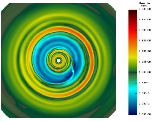
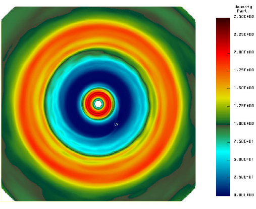
Figure 2: Perturbations of the surface density structure of the disk relative to the initial density at each point ($\Sigma(r,\theta,t)/\Sigma(r,\theta,t=0)$)for the high mass prototype simulation, mas7, in which an embedded 1$M_{\rm J}$  planet sweeps out disk matter and begins forming a gap. (top) Early in the run, prior to achieving a steady state (300 yr after the beginning of the run). (bottom) Late time, near steady state density structure (1800 yr). In both images, the boxed region $\pm$15 AU from the origin is shown. The white ovoid shape defines the region dominated by the gravity of the planet (i.e. its inner and outer extent define a distance of 1$R_{\rm H}$ from the planet).

Snapshots of our high mass prototype model are shown for early and late times of the evolution in figure 2. Figure 3 shows the azimuth averaged surface density profile at various times during the evolution. Early in the simulation, spiral density waves are excited by the planet which extend inwards from the planet’s position to $\sim 1-1.5$ AU and outwards to $\sim 15$ AU before fully dissipating. Within the first $\sim 100$ yr, a large evacuated region trailing the planet and extending nearly a third of the way around the disk has formed in the planet’s wake. A similar region extends ahead of and radially inward from the planet.

After another 2-300 yr of evolution, the evacuated regions ahead of and behind the planet have grown completely around the star and have begun to form a gap region in the disk where the surface density has decreased a factor of 3–5 below its initial value. During its formation, the gap is deepest inward/ahead of the planet and outward/behind the planet in the sense of the orbital trajectory and is not axisymmetric. Strong spiral structure is present near the planet and throughout the disk. Finally after 6-800 yr of evolution, the spiral structures decrease in amplitude, the disk becomes nearly axisymmetric and settles into a slower, secular evolution. Vestiges of low amplitude spiral structure are still present in the gap even after 1800 yr of evolution and extend inwards and outwards several AU into the higher density regions of the disk.

The gap forms quickly after the beginning of the simulation and within 600 years has grown to a 3 AU width, while the planet has migrated inwards to 4 AU from the star. When the migration stops, the density near the planet is a factor of six to eight below the initial density at 4 AU, at about 200 g/cm² near the planet and 100 g/cm² near the minimum, which is not found at the same orbit radius as the planet, but slightly further out. Later, when the gap has more fully formed, a very low density central region in the gap forms within $\pm 2R_{H}$ from the planet. Once the gap has formed, little further evolution of the disk as a whole occurs, but the surface density near the planet continues to decrease and falls to $<10$g/cm² at $t=2400$ yr. The matter in the outer disk is left behind by the migration of the planet inward, and the planet’s influence on it becomes progressively smaller. The gap’s outer edge is thus much more shallow than its inner edge, to which the planet moves progressively closer until its migration stops.

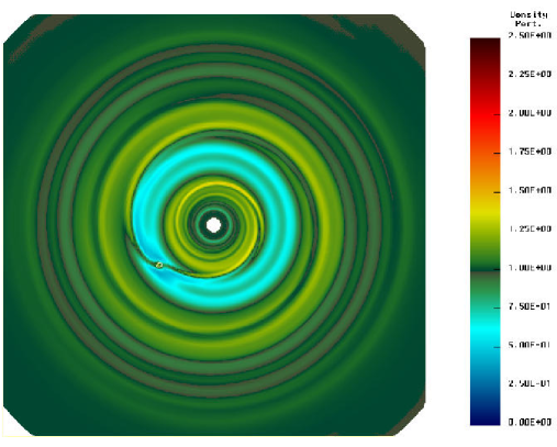
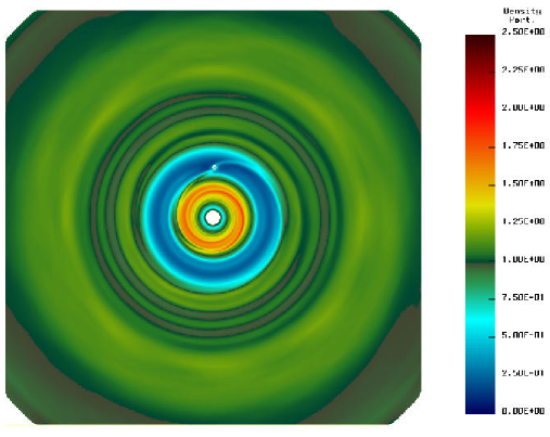
Figure 4: Perturbations on the surface density structure of the disk for the low mass prototype (simulation mas3) after being perturbed by a low mass planet (0.3$M_{\rm J}$) traveling through the disk. The times from the beginning of the run are 300 yr (top) and 1800 yr (bottom). In comparison to the high mass prototype, spiral structures and perturbations are much lower in amplitude. As in figure 2, the white ovoid shape defines the region dominated by the gravity of the planet (i.e. its inner and outer extent define a distance of 1$R_{\rm H}$  from the planet).

The evolution of the low mass prototype is shown in figure 4. As for the high mass prototype, the planet builds spiral structure ahead of (behind) its azimuthal position in the disk and which is inward (outward) from its radial position. The spiral structure is of much lower amplitude in this case but remains present for the duration of the simulation. It extends radially inward from the planet to 1.5 AU and outward to 15 AU. In this model, as for the high mass prototype, secondary, $m=2$ and $m=3$ symmetry patterns are easily visible in addition to the primary spiral pattern which intersects the planet’s position in the disk.

Gap formation occurs more slowly in this simulation and the gap does not reach the depth necessary to stop the planet’s motion (see section 4.2) during the first $\sim$2000 yr evolution, but after 3000 yr of evolution, it does build a deep enough gap and rapid migration stops. Over the course of the run the planet migrates inward about 2 AU, and when the migration slows, the surface density in the gap has decreased to a factor $\sim 4-5$ below the initial density (figure 5). The outer disk density profile remains relatively unperturbed during the evolution.

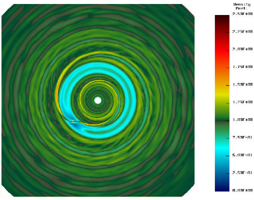
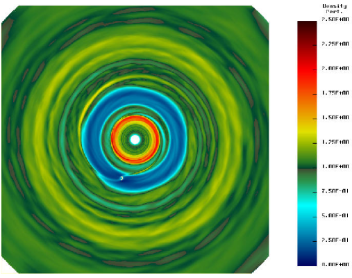
Figure 6: Perturbations on the surface density structure of the disk for the high resolution prototype (simulation Sof7) after being perturbed by a low mass planet (0.3$M_{\rm J}$) traveling through the disk. (top) Early in the run, after 300 yr of evolution. (bottom) Late in the run (1800 yr). In comparison to the low mass prototype, spiral wave structures are visible much further from the planet and the gap is slightly deeper and wider. As in figure 2, the white ovoid shape defines the region dominated by the gravity of the planet (i.e. its inner and outer extent define a distance of 1$R_{\rm H}$ from the planet).

In order to make direct comparisons to our standard resolution runs, we ran a high resolution simulation with the gravitational softening parameter increased to $\epsilon=2.0$ (making it identical in absolute size to the low mass prototype). We show early and late time snapshots of the evolution of a run like our low mass prototype in figure 6 and azimuth averaged surface density profiles in figure 7. Qualitatively, many of the features in figures 4 and 6 are quite similar in the region close to the planet. In both examples, spiral waves excited by the planet are visible inward and outward from the planet’s position, a gap forms around the planet and spiral structures extend into this gap region to the planet.

There are also important differences between the two simulations. In the high resolution prototype, density perturbations are nonaxisymmetric until much later times in the evolution and small amplitude, high $m$ spiral structures are visible in the horseshoe region of the gap. Spiral structure extends much further inwards and outwards than with the standard resolution model, over nearly the entire radius range simulated. Although the spiral structure extends further, the changes that develop in the surface density profile are more concentrated into distinct regions. The gap becomes deeper more quickly and the region just inward of the $m=2$ inner Lindblad resonance develops a large density enhancement as matter piles up there. The differences that exist are due primarily to changes in the breakdown point (i.e. which $m$ patterns propagate some distance, rather than damp immediately upon formation) of our local damping assumption and few physical conclusions can be made about them.

At higher resolution, some wave components excited by the planet are able to reach both the inner and outer grid boundaries with a small but non-zero amplitude. Except to produce a perturbation on the surface density profile there (figure 7), we do not believe this boundary interaction strongly affects the gap formation process or the planet’s migration through the disk. Since the waves are already very low amplitude at the boundary, their reflections do not travel far before being completely dissipated.

Perturbations of similar magnitude, clearly unrelated to boundary interactions, are present in both the high and low mass prototype simulations. In these runs, the inner disk develops a much flatter radial profile than it initially has. The flattening in the profile is due in part to the migration of mass inwards which was originally in the gap region, but is also due to the outward migration of some material in the inner disk. The location at which this is most apparent ($\sim 1.0-1.5$ AU–see the early time panels of figures 3 and 5) corresponds to that at which the inner spiral structure decays to zero amplitude (see Paper II  ).

We were not able to isolate the exact physical or numerical origin of the locally outward migration. However, we believe it is no coincidence that the behavior is most visible at the same location as the decay to zero amplitude of the spiral structure. While the largest fraction of gravitational torque interaction is generated by the planet near its Lindblad resonances, a small, but non-zero torque contribution is generated far from the resonance. This contribution oscillates in sign, successively adding or subtracting angular momentum from the wave as it propagates away from the planet. Wave decay implies a large asymmetry between crests and troughs of successive radial waves and the torques they are responsible for, so that the portion of this locally generated torque realized is not symmetric from crest to trough of one wave form to the next, perhaps leading to the observed effect.

4.2 Evolution of the planet’s orbit under the disk’s influence

Because of the efficient transfer of angular momentum between the planet and the disk, a massive planet experiences large dynamical torques and suffers rapid inward migration. In some cases, its orbit radius decreases by a third after only a few hundred years of evolution. In figure 8, we show the radial trajectory of the planet from our three prototype simulations discussed above. After a $\sim 100$ yr period in which the planet first builds spiral structures, the high mass prototype (top panel) produces a near constant migration rate for the next 500 yr. After 600 yr, when the planet has reached an orbit radius of about 3.6 AU, the migration rate decreases to near zero. Finally, the trajectory changes to a slow outward migration as the planet’s position relative to the gap center equilibrate.

For the low mass prototype, the migration proceeds for most of the run at a slowly decelerating rate. The migration begins to slow more strongly after 2000 yr and, after 2700 yr, stops when a deep enough gap forms. The version of this simulation without disk self gravity does not decelerate and stop. Instead it migrates at a much faster rate so that within 1000 yr has migrated more than 2 AU from its initial orbit radius. Shortly thereafter (not shown on the plot), it begins to accelerate as it moves into higher surface density regions closer to the star and after 1200 yr, it impacts the inner boundary of our grid. Similar behavior is observed in the simulations with very low mass planets including disk self gravity (e.g. simulation mas1 with $M_{\rm pl}$=0.1$M_{\rm J}$).

In contrast, the high resolution prototype (with disk self gravity) is characterized by a much slower migration rate than its standard resolution counterpart. Over the entire duration of the simulation the planet migrates only about 0.6 AU, compared to the $\sim 2$ AU migration that the standard resolution simulation suffers. The migration also slows and stops due to the differences in the character of the gap that forms. On the other hand, the version without disk self gravity suffers an extremely rapid migration rate–faster than either its low resolution counterpart or either of the two simulations including self gravity. After only $\sim$300 yr, it has migrated 2 AU through the disk and very quickly thereafter accelerates still faster and begins to interact with the inner grid boundary.

In none of the four simulations with 0.3$M_{\rm J}$  planets, are migration rates obtained that are identical to any of the others. Among the four models, we vary two parameters: the presence/absence of disk self gravity and sensitivity to the 2d mass distribution (via the varying grid resolution). Looking at the two pairs of models with and without self gravity at the same resolution (i.e. the pairs mas3/nosg and Sof7/Nosg), we observe that in both cases the migration is faster without self gravity than with it. This is interesting because any variation at all runs counter to the expectation that self gravitating disturbances should be largely suppressed, since the Toomre stability parameter is $Q>5$ everywhere. On the other hand, looking at the two pairs of models that vary grid resolution with or without self gravity (i.e. the pairs mas3/Sof7 and nosg/Nosg), we do not observe a consistent pattern: with self gravity migration is slower with higher resolution but without self gravity, migration is faster with higher resolution.

It is significant that the rate differences in the latter case cannot be due to changes in the dissipation between the models. Such differences would produce large changes in the surface density profile, as shown in figures 5 and 7. However, during the period the migration rates are calculated, the gap has only begun to form. Its structure is thus relatively undifferentiated from the others and will have little effect on the torques on the planet. Therefore we can conclude that the origin of the rate differences lies in physically meaningful quantities: in one case the effect self gravity and in the other the mass distribution near the planet.

4.3 Dependence of the migration rate on planet mass and disk mass

We expect the migration of a planet through the disk to depend both on the mass of the planet and the mass of the disk in which the planet evolves. The Type I migration rate (expressed as a migration velocity by Ward (1997a)) is directly proportional to the planet mass and the disk surface density

$${{\dot{a}}\over{a}}\propto M_{\rm pl}\Sigma,$$ (5)

given that only Lindblad resonances are important for the migration. We have run a series of simulations varying planet mass (designated mas in table 1) in order to test this proportionality. Further, to test the sensitivity of the migration rate to the mass surface density, we have run a series of simulations (designated dis) which vary the assumed disk mass. With identical grid dimensions (inner and outer boundary radii), disk mass and surface density are directly proportional, so that the proportionality in equation 5 still holds.

In figure 9, we show the migration rates fit for simulations with different planet masses. The rates shown are valid for the period for which the migration rate is constant in that simulation (see figure 8). In other words, the fit is obtained over the period for which the migration can be considered ‘Type I’, and the planet has migrated less than $\sim$2 AU from its original orbit radius. The rates are nearly independent of planet mass–the expected linear trend is not present. The migration rate for the simulation with $M_{\rm pl}$$=4$$M_{\rm J}$ is plotted to complete the full series, but should be disregarded since it was affected by a numerical error (see appendix A).

The only significant feature in figure 9 for planets below 2$M_{\rm J}$  is a small ‘knee’ in the slope and flattening in the rates above 0.5$M_{\rm J}$. This feature may be explained by a close examination of figures 2, 4 and 6, which shows that the perturbation amplitudes have reached 20% or more, so that for these masses the planet is essentially driving the waves to saturation so that the linear theories no longer apply. Furthermore, at such high planet masses, the gap formation occurs so quickly that a truly Type I migration epoch, with an unperturbed disk, may not exist for a period long enough to obtain a well defined migration rate.

Such a massive disk as is assumed for the simulations in figure 9 may only be appropriate early in the disk lifetime, while the planet may grow to such large masses only much later. Figure 10, shows the migration rates determined for a planet with mass 0.3$M_{\rm J}$, but with lower disk masses, between $M_{\rm D}$=0.01 and 0.05$M_{\odot}$. We find a factor three speedup in the migration rate occurs over a factor five increase in disk mass, which while still appreciable is less than the linear dependence we expect from equation 5. We note the proportionality is shallower at higher disk masses than at lower, perhaps indicating that the interactions have begun to saturate at the higher disk masses. We conclude that the expected linearity is only partially recovered in these models.

In all cases, both for varying planet mass and for varying disk mass, the fitted Type I  migration rates are very rapid: more than 0.5 AU per thousand years, and usually about 1 AU per thousand years. Planets with masses greater than 0.3$M_{\rm J}$  begin with very rapid migration rates, but within 3000 yr or less, build a deep gap where little disk matter remains. This gap slows their migration rate because the large dynamical torques acting on the planet decrease. If they remain in a Type I  migration phase, planets less than 0.3$M_{\rm J}$  would impact the star in only a few $\times 10^{3}$ yr. Lower disk masses will slow this process and will reduce the planet mass sufficient to open a gap, however an important point to note is that there is a critical region in phase space in which the planet is vulnerable to rapid migration and in which gap formation occurs too slowly to halt the migration. In order to survive, a planet must gain mass quickly enough to traverse this Type I  migration region of parameter space more quickly than it migrates through the disk.

For a 0.05$M_{\odot}$  disk, the phase space of planet masses which undergo continuous Type I  migration region is defined from above by the condition that the planet mass be less than 0.3$M_{\rm J}$. The region will also be defined from below in the sense that below some mass, a planet will no longer couple strongly to the disk via gravitational torques and its migration will be slow. The result shown in figure 9 show that a 0.1$M_{\rm J}$  planet is already well above this onset mass in a 0.05$M_{\odot}$  disk. We have not attempted to outline the parameter space further, either for planet masses below 0.1$M_{\rm J}$  or for lower disk masses, because of the limitations imposed by our coarse resolution. At our standard resolution for example, the Hill sphere of a 0.1$M_{\rm J}$  planet is about the same size as two grid zones. As we will see in section 4.5, resolving the mass distribution on this size scale is critical for determining the true migration rate.

4.4 The transition from Type I  to Type II  migration

The formation of a gap eventually causes the migration to slow and, when it gets deep and wide enough, stop. This condition defines ‘Type II’ migration, where the migration is tied to the viscosity of the disk rather than to dynamical processes like spiral wave generation and gravitational torques (‘Type I’ migration). The arguments and derivation of the Type I  migration time scale in equation 5, were also used in Ward (1997b) to determine the conditions for the transition from Type I  migration to Type II migration, at a mass he refers to as the ‘Shiva mass’ whose definition is:

$${{M_{S}}\over{M_{*}}}\approx 2\alpha_{SS}^{2/3}\left({{M_{*}}\over{\Sigma r^{2}}}\right)^{1/3}\left({{c_{s}}\over{r\Omega}}\right)^{3},$$ (6)

where $M_{S}$ is the Shiva mass, $\alpha_{SS}$ is the Shakura & Sunyaev (1973) viscous parameter and the radius, $r$, is position of the planet. However, we saw in the last section that the predictions of equation 5 are only partially recovered in the simulations and therefore cast doubts on the derivation of the Shiva mass as well.

Indeed, some discrepancy exists. Given the parameters of our simulations (section 2.1), we expect the Shiva mass to be $M_{S}\approx 1.4\alpha^{2/3}$$M_{\rm J}$, which requires a very large value $\alpha\sim 0.1$ to match the 0.3$M_{\rm J}$ transition mass seen in our simulations. With more usual values of $\alpha=0.01$ or 0.001, we derive $M_{S}\approx 20$$M_{\oplus}$  or 4.5$M_{\oplus}$, respectively, far lower than in our simulations. In order to explore the discrepancy with theory, we determine empirically the approximate disk conditions that define the boundary between Type I  and Type II migration for a given system as it evolves forward in time.

First, we attempt to gain some qualitative insight from figure 8. Looking specifically for a moment at the high mass prototype, we see that the migration begins to slow after about 5-600 yr of evolution, and essentially stops after $\sim 900$ yr. Comparison with figure 3 shows that the planet begins to slow it migration when the gap is 3 AU wide and has surface density $\Sigma_{gap}\sim 200$ g/cm². The transition is complete and little further migration occurs when the system has evolved for 900 yr, and the surface density is $\Sigma_{gap}\sim 100$ g/cm². We see similar behavior in the low mass prototype, except that the time scale is extended to about 1800-2000 yr before the rates slows significantly and 2700 yr for it to stop, with surface densities of $\Sigma\sim 3-400$ g/cm² and $\Sigma\sim 300$ g/cm² at 2000 and 3000 years, respectively.

Disks with mass density at or below these values and planets as massive as 0.3$M_{\rm J}$  will have already undergone a transition to Type II migration, so that migration will be slow. The results of our ‘dis’ series of simulations did indeed confirm that 0.3$M_{\rm J}$ planets embedded in less massive disks (i.e. with $\Sigma\sim 2-400$ g/cm²) migrate only a few tenths of an AU from their initial orbital position before they form gaps. With a surface density distribution like that in our simulations (i.e. $\propto r^{-3/2}$), a value of 200 g/cm² at 4 AU corresponds to a disk mass of $M_{\rm D}$$\approx$0.01$M_{\odot}$ between 0.5 and 20 AU. With a shallower distribution ($\propto r^{-1/2}$) the implied disk mass is $M_{\rm D}$$\approx$0.02$M_{\odot}$, both of which are comparable to the minimum mass solar nebula required to make the planets in our own solar system. We conclude that minimum mass solar nebula disks with embedded planets of 0.3$M_{\rm J}$  or larger will exhibit Type II migration. Lower mass planets may also successfully make the transition to Type II migration in a minimum mass solar nebular as well, however we have not studied that question in detail.

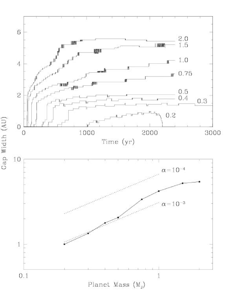
Figure 11: The gap width for the mas series of simulations. In the top panel the gap width is shown as a function of time as the simulation proceeds. The curves are jagged because the gap width is measured as a discrete number of grid zones. Each number shows the planet mass (in $M_{\rm J}$) corresponding to each curve. The bottom panel shows the final gap width as a function of planet mass. The inner and outer gap edges are defined as the radii at which the surface density drops to a factor of two below the initial surface density. Except for the $M_{\rm pl}$=0.2$M_{\rm J}$ model where we take the value at time t=2000 yr, the gap width is defined as the width at the conclusion of the simulation, usually 2400 yr. The dotted curves define the gap width derived from eq. 7 and assuming a viscous coefficient $\alpha_{SS}=10^{-3}$ and $10^{-4}$ as marked.

A more quantitative measure of our results is the gap width as a function of planet mass. In the top panel of figure 11, we plot the width of the gap vs. time for each of the mas series of simulations. Initially unperturbed disks will form gaps within a few hundred years of the evolution, when perturbed by the passage of a planet with mass $\geq 0.3$$M_{\rm J}$. After its initial fully Type I  phase, the gap forms and widens quickly to near its final value, then (for the higher planet masses) slowly increases further for the duration of the simulations. In addition, if we compare figure 11 to figure 8, we see that the formation of a gap does not necessarily imply an immediate halt to the migration. Simulations with planets $<0.3$$M_{\rm J}$ enter the transition to Type II  migration temporarily, but do not exit. Instead, they return to the fully Type I  phase as they move inward into higher density regions of the disk, finally impacting the inner grid boundary.

The analytical work of Takeuchi et al.  (1996, hereafter TML) predicts that the gap width will be approximately

$$\delta r\approx 0.9a_{\rm pl}\left({{q^{2}}\over{\alpha_{SS}h_{0}^{2}}}\right)^{1/3},$$ (7)

where $q$ is the mass ratio between the planet and star and $h_{0}$ is the dimensionless scale height of the disk, and assuming that the gap is relatively narrow. Since we assume separate mechanisms for the dissipation of waves and for viscous spreading (section 3.1.1), rather than a single mechanism of constant magnitude ($\alpha$ value) for all dissipation sources, correspondence between our results and equation 7 would appear to be difficult to arrange. However, since we have assumed local damping, we can neglect spatial variation in dissipation, allowing us to substitute a single, unknown value for the dissipation cast as an $\alpha_{SS}$ model. This will allow us to establish the veracity of the theoretical model, given only correspondence with the proportionality.

In the bottom panel of figure 11 we show the gap width as a function of planet mass, measured at the end of each simulation when the evolution and gap structure had reached their near steady states. Also shown are the gap widths predicted by eq. 7, assuming a scale height of $h_{0}=0.045$ and a planet orbit radius of $a_{\rm pl}=$4.5 AU. Over the range between 0.2 and 1.0$M_{\rm J}$, the gap width derived from the simulations is slightly steeper than the predicted proportionality of $M_{\rm pl}$^2/3. We believe that the difference is due mainly to the spatial variation of our numerical dissipation. Overall, the differences are small and the agreement between theory and simulation is good.

Although we cannot specify a single input value of $\alpha_{SS}$, we can use equation 7 along with the results of our simulations to provide a useful a posteriori check on the overall background (non-wave) dissipation in PPM. For our standard resolution, figure 11 shows that the gap sizes correspond to $\alpha\lesssim 10^{-3}$. While this value puts our simulations well within the range of values in general use for circumstellar disks, it is in conflict (by a factor of 100) with the value estimated from equation 6 and the 0.3$M_{\rm J}$  critical gap opening mass obtained from the same simulations.

The origin of the conflict lies in our separation of wave dissipation from other forms. The gap width $\alpha_{SS}$ value (of $10^{-3}$) is based on the long term state of the system after waves have mostly decayed away. It therefore reflects the low ambient internal dissipation expected of accretion disks (section 3.1.1) and provided by PPM. On the other hand, the Shiva mass from equation 6 is derived from a much more active part of the evolution, where waves generated by the planet reach significant amplitudes for which shocks may form. As we noted in section 3.1.1, shocks are known to develop near the planet for planet’s more massive than $\sim 30$$M_{\oplus}$, so the dissipation there will be high for quite physical reasons, and correspond to a locally high value of $\alpha_{SS}$, for the times when those shocks are present.

While the strong wave dissipation implied by our local damping assumption may indeed be responsible for the two different values of the Shiva mass, that responsibility cannot be extended to the migration rate’s lack of sensitivity to changes in the planet mass. In that case, local damping neither helps nor hinders the migration until large changes in the density distribution have evolved. Since we limit our fits to the Type I  evolution period, they will not be strongly affected by the details of the wave damping and the conflict with theory remains.

4.5 The strength of dynamical interactions between the planet, its envelope and circumstellar disk

While we find very good agreement for the gap width to planet mass proportionality, the same cannot be said of the migration rate proportionalities, which were reproduced in one case and not another. Although we could show at least a close to linear dependence of the migration rate on disk mass, we did not find the expected linear dependence on planet mass. Instead the rate varied by less than a factor two over a factor 20 change in planet mass. Both the predictions of the migration rates and the gap widths are derived from the same theoretical framework, namely that the gravitational torques are generated from Lindblad resonances. Why does the correspondence fail in some cases and not in others?

When a gap has already formed and little matter remains near the planet, the assumption underlying equations 5 and 7 (that only Lindblad resonances are important) may indeed be valid, especially if the gap is wide and deep enough that interactions close to the planet are small. In the immediate vicinity of the planet, especially during the Type I phase, other interactions like corotation resonances and mass accretion may be important, each giving much larger significance to the small scale mass distribution than is assumed using equations 5 and 7.

How influential are the mass structures that form around a planet in terms of their effect on the dynamical evolution of the planet/disk system as a whole? We study this question by varying the gravitational softening parameter (see eq. 4) used to calculate the force between the planet and disk. With large softening, little significance is given to the matter near the planet, while with small softening much more significance is given. We vary gravitational softening radius between 0.1 and 4.0 times the size of one grid zone, corresponding to a physical size between 0.015 and 0.6 AU at our standard resolution of 128$\times$224 grid cells. For these simulations (designated sof in table 1), we assume the same initial conditions as for our low mass prototype simulation above.

The migration rates obtained from these simulations are shown in figure 12. The migration rate increases by a factor of about five as the softening decreases from 0.5 AU to 0.1 AU. The largest increases occur as the softening decreases to the size of the Hill radius or smaller. As the softening decreases below $\epsilon=0.5$, the magnitude of the migration rates decreases to zero, as the planet becomes unphysically bound to a single ring of grid zones.

For the physically relevant range of softening parameters ($\gtrsim 0.1$AU) studied, we can make the important conclusion that the distribution of disk matter within 1–2$R_{\rm H}$ (i.e. with both very similar orbit radius and orbital phase as the planet) of the planet plays a critical role in determining its orbital evolution and fate during its Type I  migration phase. This is a stronger conclusion than that made by one dimensional analyses, which are able to conclude only that the radial region within a few $R_{\rm H}$  is important. We base it both on the large increase in migration rates with decreasing softening and our earlier (section 4.2) finding that the migration rate is sensitive to the grid resolution employed in the simulations. Although our simulations are two dimensional, the conclusion is general in the sense that it includes both the two and three dimensional mass distribution, since the softening affects torques on a spatial scale very similar to the disk scale height.

5 Discussion and Comparisons to Other Work

In this section we attempt to compare our results with some of what has gone before, to place them in context. In terms of the physical model, while we have employed a deliberately simplistic thermodynamic treatment, we know of only one study other than our own (Meyer-Vernet & Sicardy, 1987), after GT79 which includes disk self gravity in an analysis of planet migration. Even there, the discussion is of the properties of wave generation and propagation of disturbances in the disk, rather than on the consequences for the planet. Explicitly stated or not, the assumption made in studies of planet migration so far has been that self gravity would contribute only negligibly to the migration since a disk with as low a mass as ours should be stable (i.e. Toomre $Q>>1$). Given its dramatic effect in our simulations, this assumption must be discarded in future analyses.

What is the origin of the large rate changes when disk self gravity is included? Although the answer to this question is beyond the scope of our work here, where we have made only relatively qualitative comparisons of our results to analytic predictions, we may be guided in our speculations by Ward (1997a). He shows that pressure forces will cause slight shifts in the rotation curve of the disk, relative to purely Keplerian flow, causing the resonance locations themselves to shift. These shifts can be responsible for very large changes in the net Lindblad torque on the planet because that torque is a sum of two large terms of opposite sign. Disk self gravity will produce similar shifts and we will find in Paper II   that in fact resonance shifts due to inclusion of disk self gravity can cause large changes in the gravitational torques, so they may be responsible for at least some of the observed sensitivity.

Previous numerical studies of disk with embedded planets fall into two general categories. First, there are studies like our own that begin with an unperturbed disk containing a planet (e.g. Bryden et al. , 1999; R. P. Nelson et al. , 2000) and second, studies that begin with an already formed gap around the planet (Lubow, Siebert & Artymowicz, 1999; Kley, 1999; Kley, D’Angelo & Henning, 2001). In general, the previous studies have focused on planets with mass 1$M_{\rm J}$ or larger and a single disk mass (a ‘minimum mass solar nebula’), during the gap clearing process and following Type II migration epoch. In many instances they suppress planet migration in order to explore gap formation and mass accretion processes in isolation. The period of gap clearing is common to both our study and the previous studies and it is on this basis that we compare our results to theirs.

5.1 Comparisons to semi-analytic and numerical ‘$\alpha_{SS}$’ models

We find that planets more massive than $\sim 0.3$$M_{\rm J}$  can open a gap sufficiently wide and deep to halt their dynamical migration through the disk (i.e. transition to Type II  migration), even for relatively massive ($M_{\rm D}/M_{*}$=0.05) disks. The critical planet mass of 0.3$M_{\rm J}$  agrees very well with a result from Lin & Papaloizou (1993) that only planets with $M_{\rm pl}$/$M_{\odot}$$>3(H/r)^{3}$ could form gaps, but provides the additional information that there is enough time for the gap to open before the planet is lost by accretion onto the star, even if the system starts from the condition that no gap has yet started to form.

The gap sizes produced in our simulations are somewhat wider than the values quoted by Bryden et al.  (1999) (a half width of $\sim 0.2a_{\rm pl}$ for a 1$M_{\rm J}$  planet, compared to our value of $\sim 0.5a_{\rm pl}$), mainly because of a difference in the definition of a gap. While both the TML and Bryden et al.  (1999) derivations follow from the same physical arguments and produce the same proportionalities, it is not clear what factor should be used in order to produce an equality, because of the ambiguity about what point in the evolution that equality should signify. The usefulness of a gap width relation such as equation 7 is therefore limited. While we used the TML definition in section 4.4, it is clear that forming a gap of a given width and the end of rapid migration are not equivalent statements. On the other hand, the Bryden et al.  (1999) definition produces a time scale for gap opening proportional to the width to the fifth power, so a small error in the width (through e.g. a mis-estimation of $\alpha$ or the disk scale height) will have large consequences on the predicted time scale, perhaps leading to the incorrect conclusion that a planet might or might not be accreted by the star when in fact the opposite result is the case.

On one level, our result that the critical planet mass for opening a gap is $\sim 0.3$$M_{\rm J}$  is interesting because it validates the initial conditions of the many models beginning with a massive planet and an already formed gap. However, it does not address the question of how that initial condition came to pass–lower mass planets do not form gaps and instead continue to migrate rapidly. Unless some mechanism exists by which they can avoid such rapid migration, they will be accreted by the star, completing the ‘Shiva’ scenario of Ward & Hahn (2000). Moreover, the Shiva mass is derived while neglecting disk self gravity, while our simulations include it. While we have not investigated the exact transition mass in simulations of non self gravitating disks, it is clearly much higher than 0.3$M_{\rm J}$, making its value even more inconsistent with the theory.

The gap opening mass from our simulations is inconsistent with not only the predicted Shiva mass of $\lesssim 10-20$$M_{\oplus}$  discussed in Ward & Hahn (2000) but also the value obtained from estimating an $\alpha_{SS}$ value from the gap widths themselves (figure 11). This conflict exposes an important shortcoming in many analytic theories of migration. In nearly all such models, the magnitude of dissipation (ordinarily a single $\alpha_{SS}$ value) defines all of the dissipation in the system at every point, effectively separating the assumption of local wave damping from the magnitude of the dissipation supposed to cause it. Given the importance of spatially and temporally varying dissipation processes like shocks in models of planet migration, this separation is quite dubious. In our models, we have retained both a low ambient dissipation and the local damping assumption in a self consistent manner, leading to the conflict. In order to retain self consistency, analytic theories must also allow for this separation.

5.2 Sensitivity of the results to spatial resolution

Based on the partial agreements and disagreements with theory (section 4.5) and on the high sensitivity to the mass distribution (i.e. the resolution and the gravitational softening), we made the physical conclusion that the two and three dimensional mass distribution within 1–2$R_{\rm H}$  of the planet is very important for determining its fate.

In terms of the radial distribution of matter, requiring a very well resolved mass distribution is far from a new conclusion. A large fraction of the torque comes from higher order ($m\sim 10-20$) Lindblad resonances located about a disk scale height inward and outward of the planet. In part, the added significance in this work is that the sensitivity extends to the azimuth and vertical coordinates as well. A previous shearing sheet calculation (Miyoshi et al. , 1999) showed that allowing for three dimensional structure near the planet can cause a factor $\sim 2.5$ decrease in the magnitude of the torques relative to two dimensional calculations, but because their calculations modeled only a small region around the planet it was unclear how the results might translate into more global models. A contrasting result with global 3d simulations (Kley, D’Angelo & Henning, 2001) found little difference between rates determined from 3d calculations and from previous two dimensional versions.

In our simulations, the 1–2$R_{\rm H}$  spatial scale is resolved by only a few zones, which gives a relatively coarse picture of the mass distribution there. Indeed, the sensitivity of our results to resolution is a major factor in making the conclusion in the first place. Given the variation in migration rates for physically identical simulations of different resolution, we must conclude that our resolution is not high enough to determine a well converged value for the migration rates of the planets. The resolution employed in our models is quite similar to that employed in many other works (typically between 1 and 25 $\times 10^{-3}$ AU², though with grid spacings that vary substantially between works), and we would expect that many of them are affected by the same factors affecting our own.

What resolution is sufficient? The models of Lubow, Siebert & Artymowicz (1999) resolve the Hill sphere of a 1$M_{\rm J}$ planet in two dimensions with about 250 zones, using a variably spaced grid so that resolution close to the planet is high. This is a factor $\sim 5-6$ better spatial resolution of area than our high resolution models (which resolve the Hill radius of a 0.3$M_{\rm J}$ planet with $\sim 20$ zones), corresponding to a factor $\sim 2.5$ better linear resolution. They find little variation in the flow pattern around the planet with varying softening parameter, so it seems likely that their resolution is sufficient to resolve the gravitational torques as well. Therefore, unless the migration rates change by a large factor with an additional factor $\sim 2-3$ in linear resolution beyond our high resolution models, our rates will also not suffer from a large error.

Since many of the concerns regarding an incompletely converged migration rate are relevant both to this paper and to Paper II  , we will address the veracity of conclusions made in both papers here. In most cases, although undesirable, the lack of full convergence does not greatly diminish the value of our conclusions because they have been based not on the value the migration rate, but rather on its variation with various physical and numerical parameters. While a systematic error in the magnitude of various quantities (gap width and migration rate as a function of planet mass, or migration rate as a function of disk mass) may be present, the conclusions regarding the proportionalities remain unaffected because each simulation in each series was done at the same resolution, meaning that any systematic effects will affect each in the same way. Our finding that disk self gravity was important for the evolution will also be unaffected, as will our finding in Paper II  that that the rate of accretion onto a planet is dominated by the small scale conditions very close to it rather than by the large scale disk morphology.

The remaining concerns are with respect to the magnitudes of the migration rates (or equivalently, the torque magnitudes) and through them, of quantities like the Shiva mass and the mass accretion rates required for the planet’s survival. Two conclusions may be affected by such variation. First, the conflict between torques from theory and simulation (Paper II  ) become smaller if the migration is in fact faster. Since the migration rates and torques instead decreased with higher resolution (at least for the situation most relevant to real systems–with disk self gravity included), the torque magnitude conflict either remains or is understated in our work.

Second, with a slower migration rate, the Shiva mass and the lower bound of the accretion rate onto the planet derived from that rate in Paper II  would each be lower. Based on these two values, we made the conclusion that the early stage of planet formation was inconsistent with both a core$+$circumplanetary disk and a static spherical envelope morphology. If the true Type I  migration rates are a factor ten slower than those shown in figure 9 (i.e. $\sim 10^{-4}$ AU/yr), the conclusion will remain valid, though weakened, since the statement was based upon a very conservative model for the planet’s disk (that its mass was relatively small). It would be nullified in the unlikely case that the true Type I  rates were a factor of one hundred slower ($\sim 10^{-5}$ AU/yr).

Appendix A Numerical issues concerning the point mass force calculation

In this appendix, we examine the numerical influences of the softening radius and grid resolution on the force calculation responsible for determining the planet’s trajectory, in order to understand any systematic errors that we may make and the requirements needed to obtain reliable results. The gravitational force between the planet and the disk must be modified from its true form because the matter in the disk is resolved only as a set of small zones in a grid. Without modification, a close encounter with the center of a single zone will cause an effectively infinite and unphysical force to be calculated. Further, when the trajectory of the point mass is along a grid direction, the force calculation will be systematically slightly different when it is located near the zone centers, compared to that when it is near the zone interfaces.

In order to avoid these kinds of errors, we would like the region over which the force is modified to be large, so that any single grid zone (or azimuthal ring of zones) does not produce an unduly large influence on the trajectory. On the other hand, the physical effect of a large softening parameter is to blur or ‘turn off’ the mutual interaction between the planet and disk exactly where it may be the strongest, and may lead to an incorrect model of the evolution. Therefore, we would also like the modified region to be as small as possible in order to correctly calculate the force due to the disk mass close to the planet.

To address both of these requirements, we use direct summation of the force between the planet and each grid zone using the Plummer force law as defined in eq. 4. This form allows the softening radius, $\epsilon$, to be chosen as a constant fraction of the zone size that the planet is in, but still allows the freedom to choose the value of that fraction differently in different simulations. We also experimented with a constant softening parameter, but found no difference between those results and with those using a constant fraction of the current zone size, since the force is proportional to $1/\epsilon^{2}$ and radially adjacent zones change in size by $<$2%.

We show the trajectories of the planets in a series of simulations that varied the softening parameter in figure 13. With very large softening values we find that the planet migrates only very slowly through the disk. In this case, only relatively distant parts of the disk are able to influence the trajectory of the planet since the softening strongly suppresses the gravitational forces from nearby material. As the softening value decreases, the migration rate increases as the forces due to the disk mass close to the planet approach their unsoftened values. However, this influence ultimately becomes incorrectly modeled because of the finite resolution of the grid. For softening values $\epsilon\sim 0.5-0.75$, the radial trajectory shows clear evidence of a stair step pattern, as the planet passes inward into the influence of successive rings of grid zones. When the softening value reaches less than half the size of one grid zone, the influence of a single grid zone or a single azimuthal ring of grid zones dominates the gravitational force on the planet, unphysically binding its orbit to that ring so that its migration rate drops to zero.

For simulations with higher mass planets or higher grid resolution, the situation reverses: The migration rates obtained when this occurs are very rapid, generally faster than 1 AU/100 years. The most massive planet we simulated (ms10, 4$M_{\rm J}$) migrated inward to half it’s initial orbital radius in 60 years, then stopped due to the formation of a gap and the build up of disk matter between it and the inner grid boundary. This behavior is not the inertial migration regime as discussed by Hourigan & Ward (1984) and Ward & Hourigan (1989), but rather a numerical effect brought about by the unphysical concentration of large amounts of matter in only one or a few grid zones very near the high mass planet, as it tries to form an ‘atmosphere’. This unphysically high density causes the force on the planet to be much greater than it would otherwise be, and is caused by our isothermal equation of state assumption which implies efficient cooling. Such assumptions break down when the optical depth becomes very high and shock and/or compressional heating become significant. We would expect each of these phenomena to occur near the planet.

While such effects are not unexpected, it is important to determine the specific pathologies and the softening values that trigger them (so as to avoid them) in our models and in our code. From these results we conclude that a Plummer softening parameter smaller than half the linear dimension of one grid zone should never be used, and that values as small of 0.75 times the size of one grid zone can be used without serious numerical defects in the simulation results for low mass planets, but at least a value of at least 1.0–1.5 should be used for higher mass planets or higher resolution simulations. In this work we will typically use a softening radius of 1.0 times the size of one grid zone.

Appendix B The numerical dissipation in PPM and its application to disk simulations

Dissipation is present in all numerical schemes for solving the hydrodynamic equations because small scale inhomogeneities are only coarsely and inaccurately resolved. In calculations done on a grid for example, unphysical mixing may occur due to the incorrect advection of mass from one zone to another. Further, no wave shorter than twice the length of one grid zone (i.e. the Nyquist wavelength) can exist, and physical effects which depend on such waves will not be included in the model. Longer waves may be present but will experience dissipation as the system evolves forward in time because of errors in the assumptions in the numerical method used to model the system.

Porter & Woodward (1994) have quantified the numerical dissipation for disturbances propagating through a grid as modeled by a PPM code. They find in an empirical study that it is steeply dependent on the ratio of the wavelength to the grid spacing. They have quantified the decay rate of a sinusoidal shear flow traveling diagonally through a two dimensional mesh and produce an empirical result that the decay rate is proportional to the third and fourth powers of the shear wavelength, $\lambda$, over the grid cell size, $\delta x$:

$${{\dot{a}}\over{a}}=-\left[A_{s}\left({{\lambda}\over{\delta x}}\right)^{-3}+B_{s}\left({{\lambda}\over{\delta x}}\right)^{-4}\right]{{u_{0}}\over{\lambda}}$$ (B1)

where $u_{0}$ is the initial velocity amplitude of the shearing wave through the grid. $A_{s}$ and $B_{s}$ are the empirically derived coefficients reproduced in Table 2 from Porter & Woodward (1994). For different advective Courant numbers (defined as $C=\delta t/\delta x\times v$, where $\delta t$, $\delta x$ and $v$ are respectively the time step, the grid size and the fluid velocity through the grid). Dissipation for a fluid shearing in a direction parallel to the grid direction will be lower.

In the context of Jovian planet migration, we expect from analytic studies that waves of many different wavelengths will be excited by the passage of the planet through the disk, and propagate in both the radial and azimuthal directions. The azimuthal wavelength of a given wave will be $\lambda_{az}=2\pi r/m$, where $m$ is the azimuthal wavenumber. The wavelength of the radial component will be a function of radius and will be dependent on the local conditions, relative to the resonances in the disk. In general, the radial component of a given wave will have much shorter wavelength than the azimuthal component and be less well resolved. (Note that this is in essence a statement of the ‘tight winding approximation’). Therefore the radial component of the wave will contribute the dominant source of the numerical dissipation of the combined pattern. Following the discussion in Lin & Papaloizou (1993), the damping of radial waves in the disk will be proportional to $e^{-\nu k^{2}t}$. Stated another way, the logarithmic damping rate of the wave amplitude can be expressed as

$${{\dot{a}}\over{a}}=-\nu k^{2},$$ (B2)

where $k$ is the radial wave number, $k=2\pi/\lambda_{r}$.

We can combine equations B1, B2 and the standard Shakura & Sunyaev (1973) expression, $\nu=\alpha_{SS}c_{s}H$, into a single expression for the expression for the $\alpha_{SS}$ parameter which quantifies the numerical dissipation of wave structures in disk simulations inherent to the PPM algorithm. If we also assume that $u_{0}\approx V_{\theta}$, we obtain $\alpha_{PPM}$ as:

$$\alpha_{PPM}={{\lambda r}\over{(2\pi)^{2}H^{2}}}\left[A_{s}\left({{\lambda}\over{\delta x}}\right)^{-3}+B_{s}\left({{\lambda}\over{\delta x}}\right)^{-4}\right].$$ (B3)

Our standard resolution simulations have $r\delta\theta=\delta r\sim 0.12-0.15$ AU near the planet so that a wave with $\lambda_{radial}\sim 1$ AU will be resolved with $\sim 6-8$ zones. Assuming conditions appropriate for our simulations, we derive a value of $\alpha_{PPM}\sim 10^{-1}$, for a wave with $\lambda=1~{}AU$ located 5 AU from the star. At double this resolution (or equivalently, for waves twice as long), we derive a value $\alpha_{PPM}\sim 10^{-2}$. For the spiral waves excited by the planet, we therefore expect that wave components with $<$1 AU wavelengths (roughly equivalent to patterns with $m>10$) will be completely dissipated very near their origination.

Given equation B3, we see that the dissipation is very steeply wavelength and cell size dependent. Changing either by a factor two changes the numerical wave dissipation by a factor of $\sim 10$. In common usage however, the $\alpha$ parameter takes one or occasionally two values over the entire disk, making clear that the dissipation in PPM and $\alpha$ models, as normally implemented, have little in common. Further, equation B1 (and therefore also equation B3) is strictly valid only for isolated single wave forms. Dissipation of multiple superposed waves cannot be calculated simply as a sum of the dissipation of individual components and instead may experience little or no numerical dissipation, depending on the local flow. A conservative approach therefore requires that we use equation B3 as a guide rather than a specification.

Infinite wavelength features (i.e. axisymmetric structures) will be only weakly damped, but nevertheless remain subject to numerical mixing and diffusion. We expect numerical diffusion is small in PPM, because of the non-linear switches to detect impending diffusive behavior in the flow and correct it. Indeed, Fryxell et al.  (1991) showed that sharp features (e.g. shocks or contact discontinuities) will spread to a width of only about two zones in a one dimensional flow before PPM’s discontinuity detection switches become active and prevent further spreading.

A gap in the surface density distribution is defined by two such features, one interior to the planet and one exterior to it. The requirement that the grid be large (radially) to provide sufficient distance for spiral waves to dissipate before encountering a boundary affords us relatively low resolution in the gap region. The gap structure may therefore be affected by the numerical diffusion. We found in section 4.4, that the gap width for a 0.3$M_{\rm J}$ planet is about $1.5$ AU, so that it is resolved in our standard resolution runs by $\sim 10$ zones. This means that nearly half of the gap may be influenced by numerical diffusion. The same gap width in our high resolution models would be resolved with twice as many zones, while the numerical diffusion effects will remain limited to regions 2 zones wide. Therefore numerical diffusion and the tendency for gap closing it implies will be lower in these runs. Looking specifically at the results of section 4.4, we note that even when resolved with only $\sim 10$ zones (for our lower mass planets), the gap widths obtained from the simulations imply a numerical diffusion whose magnitude corresponds to $\alpha\lesssim 10^{-3}$, assuming the validity of the calculation for the gap width.

Table 1: Initial Parameters For Simulations

Name	Resolution	Disk Mass	Planet Mass	Softening	Duration
	($r\times\theta$)	$M_{\odot}$	$M_{J}$	$\epsilon$	(yr)
mas1	128$\times$224	0.05	0.10	1.00	2400
mas2	128$\times$224	0.05	0.20	1.00	2400
mas3	128$\times$224	0.05	0.30	1.00	3000
mas4	128$\times$224	0.05	0.40	1.00	2400
mas5	128$\times$224	0.05	0.50	1.00	2400
mas6	128$\times$224	0.05	0.75	1.00	2400
mas7	128$\times$224	0.05	1.00	1.00	2400
mas8	128$\times$224	0.05	1.50	1.00	2400
mas9	128$\times$224	0.05	2.00	1.00	2400
ms10	128$\times$224	0.05	4.00	1.00	0600
dis1	128$\times$224	0.01	0.30	1.00	2400
dis2	128$\times$224	0.02	0.30	1.00	2400
dis3	128$\times$224	0.03	0.30	1.00	2400
dis4	128$\times$224	0.04	0.30	1.00	2400
sof1	128$\times$224	0.05	0.30	0.10	1800
sof2	128$\times$224	0.05	0.30	0.30	1800
sof3	128$\times$224	0.05	0.30	0.50	1800
sof4	128$\times$224	0.05	0.30	0.75	1800
sof5	128$\times$224	0.05	0.30	1.00	3000
sof6	128$\times$224	0.05	0.30	1.50	1800
sof7	128$\times$224	0.05	0.30	2.00	1800
sof8	128$\times$224	0.05	0.30	0.20	1800
sof9	128$\times$224	0.05	0.30	0.40	1800
sf10	128$\times$224	0.05	0.30	3.00	1800
sf11	128$\times$224	0.05	0.30	4.00	1800
Sof5	256$\times$448	0.05	0.30	1.00	250
Sof7	256$\times$448	0.05	0.30	2.00	2400
nosg	128$\times$224	0.05	0.30	1.00	1200
Nosg	256$\times$448	0.05	0.30	1.00	500

Table 2: Porter & Woodward Table 1

$C_{a}$	$A_{s}$	$B_{s}$
0.0008	343.71	4444.67
0.0080	035.36	0496.68
0.0800	007.84	0107.00
0.1600	010.84	0082.52
0.3200	020.37	0023.75
0.5600	034.70	0000.00

Figure 1: Initial conditions for surface density, Toomre $Q$, temperature and dimensionless scale height $H/r$ for the disk models. The dotted vertical lines denote the inner and outer grid boundaries.

Figure 3: The azimuth averaged density structure of the disk at several times lines). The dotted line shows the initial density profile of the disk. Also shown at each time are the location of the planet (P) and three of the lowest order ($m=1,2$ and 5) Lindblad resonances induced by the planet. The thick horizontal bar on the planet’s symbol shows the extent of Hill sphere of the planet.

Figure 5: The azimuth averaged density structure of the low mass prototype simulation at several times (solid lines). The dotted line shows the initial density profile of the disk. Symbols are as in figure 3.

Figure 7: The azimuth averaged density structure of the high resolution prototype simulation at several times during the evolution (solid lines). The dotted line shows the initial density profile of the disk, and symbols are as in figure 3

Figure 8: The evolution of the planet’s orbit for the high mass, low mass and high resolution prototype models (solid curves). For the high mass prototype, rapid inward initial motion is caused by the large torques exerted on the planet as it sweeps out matter and forms a gap, but after a deep and wide enough gap develops little further motion occurs. Neither of the lower mass simulations are able to form gaps until much later in the simulations, and so continue their rapid migration through the disk for much longer times. The dotted curves refer to the simulations which omit disk self gravity. The solid lines define linear fits to the trajectory during the period of time during which the migration rate was near constant and the gap had yet to form. Small and rapid inward/outward oscillations visible in the motion are of much smaller magnitude than a single grid zone and are probably not significant. Longer period ($\sim 100$ yr) oscillations visible in the low mass prototype are artifacts of the grid structure on the trajectory.

Figure 9: The migration rate of planets with various masses. The planets for which a gap was opened and the migration rate decreased to near zero are shown with a cross, while planets that did not open a gap are shown with a filled square. Planets with masses larger than 2.0$M_{\rm J}$ were affected by numerical errors (see text) and migrated so rapidly that no gap could form and the planets fell into the star.

Figure 10: The migration rate of a $M_{\rm pl}$=0.3$M_{\rm J}$  planet through disks with various masses. Symbols are as in figure 9. For each case, the planet was able to open a gap.

Figure 12: Variation of the migration rate with different numerical softening parameters for a 0.3$M_{\rm J}$  planet. The circled point is the simulation mig3, for which the softening parameter is $\epsilon=1.0$. The vertical dotted line is the Hill radius of the planet at 5 AU, and is also the scale height of the disk there. For runs with $\epsilon<0.5$, the migration is near zero, which is a consequence of the numerical suppression of the migration by the tendency of the planet to become locked to a single azimuthal ring of grid cells.

Figure 13: The evolution of the orbit of the planet with different softening parameters, $\epsilon$ (given in units of the local grid zone size), for the gravity due to the planet. For very large softening (e.g. $\epsilon\geq 2$), the simulations produce very slow migration rates. Migration proceeds more rapidly for intermediate softening values, ($1.0\lesssim\epsilon\lesssim 2.0$). but for still smaller values ($\epsilon=0.5,0.75$), the grid structure produces a ‘stair step’ pattern in the trajectory which becomes more noticeable for smaller softening. For the smallest softening, the planet becomes locked to a single azimuthal ring of grid cells and the results become unphysical.

References

- Artymowicz (1993a) Artymowicz, P., Lubow, S. H., 1993, ApJ, 419, 155
- Artymowicz (1993b) Artymowicz, P., 1993, ApJ, 419, 166
- Artymowicz & Lubow (1996) Artymowicz, P., Lubow, S. H., 1996, ApJ, 467, 77
- Binney & Tremaine (1987) Binney, J., Tremaine, S., 1987, Galactic Dynamics, Princeton University Press: Princeton
- Beckwith et al. (1990) Beckwith, S. V. W., Sargent, A. I., Chini, R. S. & Güsten, R., 1990, AJ, 99, 924-945
- Bell et al. (1997) Bell, K. R., Cassen, P. M., Klahr, H. H. & Henning, Th., 1997, ApJ, 486, 372
- Boss (1998) Boss, A. P., 1998, ApJ, 503, 923
- Bryden et al. (1999) Bryden, G., Chen, X., Lin, D. N. C., Nelson, R. P., Papaloizou, J. C. B., 1999, ApJ, 514, 344
- Butler & Marcy (1996) Butler, R. P., Marcy, G. W., 1996, ApJ, 464, 153
- Cassen & Woolum (1996) Cassen, P., Woolum, D. S., 1996, ApJ, 472, 789
- Chiang & Goldreich (1997) Chiang, E. I. & Goldreich, P., 1997, ApJ, 490, 368
- Colella & Woodward (1984) Colella P., Woodward, P. R., 1984, J. Comp. Phys., 54, 174
- D’Alessio et al. (1998) D’Alessio, P., Canto, J., Calvet, N., Lizano, S., 1998, ApJ, 500, 411
- Fryxell et al. (1989) Fryxell, B. A., Müller, E., Arnett W. D., 1989, Max Plank Institut für Astrophysik Report #449
- Fryxell et al. (1991) Fryxell, B. A., Müller, E., Arnett W. D., 1991, ApJ, 367, 619
- Goldreich & Tremaine (1979) Goldreich, P., Tremaine, S., 1979, ApJ, 233, 857
- Goldreich & Tremaine (1980) Goldreich, P., Tremaine, S., 1980, ApJ, 241, 425
- Goodman & Rafikov (2001) Goodman, J., Rafikov, R. R., 2001, ApJ, 552, 793
- Hourigan & Ward (1984) Hourigan, K., Ward, W. R., 1984, Icarus, 60, 29
- Kley (1999) Kley, W., 1999, MNRAS, 303, 696
- Kley, D’Angelo & Henning (2001) Kley, W., D’Angelo, Gennaro, Henning, Thomas, 2001, ApJ, 547, 457
- Korycansky & Pollack (1993) Korycansky, D. G., Pollack, J. B., 1993, Icarus, 102, 150
- Korycansky & Papaloizou (1996) Korycansky, D. G., Papaloizou, J. C. B., 1996, ApJS, 105, 181
- Marcy & Butler (1996) Marcy, G. W., Butler, R. P., 1996, ApJ, 464, 147
- Mayor & Queloz (1995) Mayor, M., Queloz, D., 1995, Nature, 378, 355
- Lin et al. (1996) Lin, D. N. C., Bodenheimer, P., Richardson, D. C., 1996 Nature, 380, 606
- Lin & Papaloizou (1993) Lin, D. N. C., Papaloizou, J. C. B., 1993, In Protostars and Planets 3, ed. Lunine, J., and Levy, E., University of Arizona Press: Tucson
- Lin & Papaloizou (1979) Lin, D. N. C., Papaloizou, J. C. B., 1979, MNRAS, 186, 799
- Lin & Papaloizou (1986) Lin, D. N. C., Papaloizou, J. C. B., 1986, ApJ, 309, 846
- Livio & Soker (1984) Livio, M., Soker, N., 1984, Icarus, 208, 763
- Lubow, Siebert & Artymowicz (1999) Lubow, S. H., Siebert, M., Artymowicz, P. 1999, ApJ, 526, 1001
- Meyer-Vernet & Sicardy (1987) Meyer-Vernet, N., Sicardy, B., 1987, Icarus, 69, 157
- Miyoshi et al. (1999) Miyoshi, K., Takeuchi, T., Tanaka, H., Ida, S., 1999, ApJ, 516, 451
- Nelson et al. (1998) Nelson, A. F., Benz, W., Adams, F. C., Arnett, D., 1998, ApJ, 502, 342
- Nelson et al. (2000) Nelson, A. F., Benz, W., Adams, F. C., Ruzmaikina, T. V., 2000, ApJ, 529, 357
- Nelson & Benz (1999) Nelson, A. F., Benz, W., 1999, Proceedings of Star Formation 1999, ed. Nakamoto, T., Nobeyama Radio Observatory: Nobeyama
- Nelson & Benz (2002) Nelson, A. F., Benz, W., 2002, ApJ, submitted (Paper II )
- R. P. Nelson et al. (2000) Nelson, R. P., Papaloizou, J. C. B., Masset, F., Kley, W., 2000, MNRAS, 318, 18
- Pickett et al. (2000) Pickett, B. K., Cassen, P., Durisen, R. H., Link, R., 2000, ApJ, 529, 1034
- Pollack et al. (1996) Pollack, J. B., Hubickyj, O., Bodenheimer, P., Lissauer, J. J., Podolak, M., Greenzweig, Y., 1996, Icarus, 124, 62
- Porter & Woodward (1994) Porter, D. H., Woodward, P. R., 1994, ApJS, 93, 309
- Porter et al. (1991) Porter, D. H., Woodward, P. R., Mei, Q., 1991, International Video Journal of Engineering Research, 1, 1
- Shakura & Sunyaev (1973) Shakura, N. J. & Sunyaev, R. A. 1973, A&A, 24, 337
- Shu (1992) Shu, F. H., 1992, The Physics of Astrophysics, Volume II: Gas Dynamics, University Science Books: Mill Valley
- Takeuchi et al. (1996) Takeuchi, T., Miyama, S. M., Lin, D. N. C., 1996, ApJ, 460, 832 (TML)
- Trilling et al. (1998) Trilling, D. E., Benz, W., Guillot, T., Lunine, J. I., Hubbard, W. B., Burrows, A., 1998, ApJ, 500, 428
- Ward (1988) Ward, W. R. 1988, Icarus, 73, 330
- Ward & Hourigan (1989) Ward, W. R., Hourigan, K., 1989, Icarus, 347, 490
- Ward (1997a) Ward, W. R. 1997, Icarus, 126, 261
- Ward (1997b) Ward, W. R. 1997, ApJ, 482, 211
- Ward & Hahn (2000) Ward, W. R., Hahn, J., M., 2000, In Protostars and Planets 4, ed. Mannings, V., Boss, A. P. & Russell, S. S., University of Arizona Press: Tucson