The Evolution of Substructure in Galaxy,
Group and Cluster Haloes I: Basic Dynamics

Abstract

The hierarchical mergers that form the haloes of dark matter surrounding galaxies, groups and clusters are not entirely efficient, leaving substantial amounts of dense substructure, in the form of stripped halo cores or ‘subhaloes’, orbiting within these systems. Using a semi-analytic model of satellite dynamics, we study the evolution of haloes as they merge hierarchically, to determine how much substructure survives merging and how the properties of individual subhaloes change over time. We find that subhaloes evolve, due to mass loss, orbital decay, and tidal disruption, on a characteristic time-scale equal to the period of radial oscillations at the virial radius of the system. Subhaloes with realistic densities and density profiles lose 25–45 per cent of their mass per pericentric passage, depending on their concentration and on the circularity of their orbit. As the halo grows, the subhalo orbits also grow in size and become less bound. Based on these general patterns, we suggest a method for including realistic amounts of substructure in semi-analytic models based on merger trees. We show that the parameters in the resulting model can be fixed by requiring self-consistency between different levels of the merger hierarchy. In a companion paper, we will compare the results of our model with numerical simulations of halo formation.

1 Introduction

In the standard picture of structure formation in a universe dominated by cold dark matter (CDM), small fluctuations present in the density field at early times grow through gravitational instability. Eventually, when their amplitude is large enough, they cease expanding with the Hubble flow, collapse and virialise, forming dense, relaxed systems, or ‘haloes’. Dark matter haloes are important as sites of galaxy formation (White & Rees 1978) and of the subsequent formation of groups and clusters through hierarchical merging (Blumenthal et al. 1984). As the densest concentrations of dark matter, they are also the best places to search for evidence of decays of dark matter particles (e.g. Gondolo & Silk 1999; Blasi & Seth 2001; see Bergström 2000 for a recent review), (self-)interactions (e.g. Peebles & Vilenkin 1999; Spergel & Steinhardt 2000; see Natarajan et al. 2002 for recent observational limits in clusters), or other dark matter physics such as bosonic or scalar properties, (e.g. Goodman 2000; Hu, Barkana, & Gruzinov 2000) connections to quintessence (e.g. Wetterich 2002; Padmanabhan & Choudhury 2002), interactions with photons (e.g. Bœhm et al. 2002), or interactions with baryons (e.g. Cyburt et al. 2002). Finally, since our own galaxy should be embedded in a dark matter halo, a detailed understanding of halo substructure is essential to interpreting the limits placed by experiments to detect dark matter directly in the solar neighbourhood (e.g. Helmi, White, & Springel 2002; see Pretzl 2002 for a recent review).

Numerical simulations of structure formation predict a generic density profile for dark matter haloes (Navarro, Frenk & White 1996, 1997; Moore et al. 1998) that is in rough agreement with those inferred from X-ray and lensing observations of galaxy clusters, at least in their outer regions (e.g. David et al. 2001; Arabadjis, Bautz, & Garmire 2002; Sand, Treu & Ellis 2002; Lewis, Buote & Stocke 2002) as well as from recent weak-lensing studies (e.g. Hoekstra et al. 2002). For less massive haloes the agreement is less certain (e.g. Blais-Ouellette, Amram, & Carignan 2001; Borriello & Salucci 2001; de Blok & Bosma 2002; Marchesini et al. 2002 and earlier references therein), but on these scales the physics of galaxy formation may have played a greater role in rearranging material within haloes. Recently, the analysis of multiply-lensed quasars (Chiba 2002; Metcalf and Zhao 2002; Bradač et al. 2002; Dalal & Kochanek 2002; Keeton 2002) and of bending in the images of radio jets (Metcalf 2002) has also provided evidence that dark matter haloes contain a substantial amount of dense substructure. In the highest-resolution simulations, this substructure is seen to result from the relative inefficiency of the hierarchical merging process: when haloes merge together, their dense cores can often survive for many orbits in the resulting system, as distinct, self-bound substructure. The overall number and mass distribution of these cores, or ‘subhaloes’, is predicted to have a universal form, roughly independent of halo mass, over many orders of magnitude, both in SCDM (Klypin et al. 1999; Okamoto & Habe 1999; Moore et al. 1999; Ghigna et al. 2000) and in LCDM (Springel et al. 2001; Font et al. 2001; Governato et al. 2001; Stoehr et al 2002) cosmologies.

Although substructure accounts for only 10 per cent of the mass of an average system, because of its high density it has important implications both for galaxy formation and for models of dark matter physics. Substructure can disrupt fragile structures in galaxy haloes, such as tidal streams (Johnston, Spergel, & Haydn 2002; Ibata et al. 2002; Mayer et al. 2002) or galactic disks (Tóth & Ostriker 1992; see Taylor & Babul 2001 for more recent references). It may substantially enhance the rate of interactions between dark matter particles, increasing the annihilation signal from dark matter if it consists of WIMPS (Calcáneo-Roldán & Moore 2000; Ullio et al. 2002; Taylor & Silk 2002). It may also account for the large mass-to-light ratios measured in Local Group satellites (Mateo 1998), as well as explaining the multiple-lensing results discussed previously.

To develop tests of the nature of dark matter at high densities and on small spatial scales where its properties may be most obvious, and to predict halo structure and substructure for galaxy and cluster formation models, halo substructure must be modelled accurately down to extremely small mass scales. Weak lensing, for instance, may be sensitive to substructure on scales of $10^{3}{\rm M}_{\odot}$ (Metcalf & Madau 2001), that is $10^{-9}$ times the mass of a galaxy halo. Unfortunately, the mass resolution limit in current numerical simulations of halo formation is much larger than this. Scaled to the halo of the Milky Way, the highest-resolution simulations of haloes presently available have particle masses of a few times $10^{5}{\rm M}_{\odot}$ (Springel et al. 2001), and thus they can only resolve halo properties down to $\simeq 10^{7}{\rm M}_{\odot}$, four orders of magnitude larger than the scale required. Clearly analytic or semi-analytic techniques are required to extend the predictions of hierarchical models any further in the near future.

In a previous paper (Taylor & Babul 2001, TB01 hereafter), we developed an analytic model for the dynamical evolution of satellites orbiting in the potential of a larger system. This model includes a simplified description of dynamical friction and of mass loss due to tidal truncation and tidal heating, using a set of evolution equations based on the global properties of a satellite to modify its mass, structure and orbit over a short time-step, rather like a restricted $N$-body simulation. As a result, it is well suited to inclusion in semi-analytic models, which must follow the evolution of large numbers of systems over many time-steps without excessive computational cost. In this paper, we extend the work in TB01 to a full model of halo formation based on semi-analytic merger trees.

A key problem we will address in this paper is the treatment of higher-order substructure, that is the substructure already present in subsidiary haloes when they merge with the main progenitor of a system. The cores of subhaloes are sufficiently robust that they may survive through many levels of the merger hierarchy, contributing to the subhalo population of the final system. In previous semi-analytic models of halo substructure, this contribution has either been ignored, by treating all haloes merging with the main progenitor as single objects with no substructure (e.g. Bullock, Kravtsov, & Weinberg 2000, 2001a), or the merger trees have been ‘pruned’ of higher-order substructure by assuming that it merges on the dynamical friction time-scale (e.g. Somerville 2002). Only the model of Benson et al. (2002a, 2002b) follows higher-order substructure in detail, by integrating orbits and calculating mass loss due to tidal stripping over many time-steps. As we will show in this paper, none of these approaches are entirely satisfactory: higher-order substructure should contribute substantially to the subhalo mass function, so it cannot simply be ignored; dynamical friction is largely ineffective for satellites with less than $10^{-2}$–$10^{-3}$ of the mass of the main system (e.g. Taffoni et al. 2002), so it will not prune merger trees efficiently below this level; and following the evolution of substructure in detail at every level of a merger tree greatly reduces the speed of semi-analytic calculations.

In this paper, we propose a simple method for reducing the complexity of a merger tree, based on the patterns that appear when we follow the dynamical evolution of systems in the main branch of the merger tree in detail. Haloes falling into a larger system should lose their bound substructure as they lose mass. We use the spatial distribution of subhaloes within a system to calculate the correspondence between the relative rates for these two processes. We assume that the most recently acquired substructure is the first to be stripped off, since it is typically on more extended and less bound orbits. This gives us a precise criterion for pruning the merger tree, passing substructure on to the next level of the tree if it has spent less than a certain number of orbits in the halo of its parent. The parameters of our method are then fixed by requiring self-consistency, that is the average mass-loss rates assumed when pruning the merger trees are the same as those measured for satellites in the main halo. As a result, the method has no major free parameters beyond those introduced in TB01 to follow the evolution of individual satellites.

The outline of this paper is as follows. In section 2, we review merger-tree models and explain how we establish the basic conditions for studying satellite evolution in a hierarchical setting. In section 3, we examine the behaviour of realistic satellites in a static halo with fixed properties, using the model of TB01. In section 4, we then show how the evolution of satellites changes when we take into account the changes in halo mass, size and density profile predicted in section 2. In section 5, we outline a simple method for pruning higher-order substructure in merger trees based on these results. We summarise our results in section 6. In a subsequent paper (Taylor & Babul in preparation, paper II hereafter), we will compare the predictions of this model with the results of high-resolution simulations, study dynamical groups within halo substructure, and discuss the overall evolution of substructure with time.

Throughout this paper we consider results for a ‘standard’ CDM (SCDM) cosmology with $\Omega=1$, $\Lambda=0$, $H_{0}=h$ 100 km s^-1 where $h=0.5$, $\sigma_{8}=0.7$ and $\Gamma=0.5$, unless otherwise noted, since our primary goal is to compare our results to simulations in this cosmology. In general, we expect very similar results for LCDM, which produces a similar subhalo mass function (albeit with indications of a lower normalisation – cf. Springel et al. 2001; Font et al. 2001; Governato et al. 2001; Stoehr et al 2002), or other CDM cosmologies. Furthermore, since our method is self-calibrating, it can be used for this or other cosmologies without reference to simulations.

2 Modelling halo formation

The growth of dark matter haloes through accretion and mergers can be predicted approximately using simple statistical arguments, the so-called ‘extended Press-Schechter’ (EPS) formalism (Press & Schechter 1974; Bower 1991; Bond et al. 1991; Lacey & Cole 1993 – LC93 hereafter). The resulting analytic expressions form the basis of many of the semi-analytic models of galaxy formation that have been developed extensively over the past decade (Kauffmann, White & Guiderdoni 1993; Cole et al. 1994, 2000; Somerville & Primack 1999; see Somerville & Primack 1999 and Hatton et al. 2003 for recent reviews). In this section we will review how these methods can be used to model the growth of dark matter haloes through hierarchical merging. We will also summarise the parameters we have used to generate the merger trees considered in this paper and in paper II, and test their properties. We will then explain how the evolution of halo structural properties, mergers with other haloes, and the evolution of halo substructure can be included within this framework.

2.1 Determining halo growth rates

One can estimate the rate at which virialised haloes form and grow by considering the evolution of a spherically symmetric overdensity with some small initial amplitude (e.g. Peebles 1980). Multiplying the initial, linear growth rate by the time at which the fully non-linear solution collapses to zero radius, one finds that the collapse occurs at the epoch when the region reaches a linearly-extrapolated overdensity $\delta\equiv(\rho-\rho_{\rm c})/\rho_{\rm c}=1.686$ for the SCDM cosmology considered here. We will refer to this value as the ‘critical’ overdensity, $\delta_{\rm c}$, hereafter.

This leads to a particularly simple method for identifying regions that will virialise at some later time – the Press-Schechter approach (Press & Schechter 1974). If one considers the density field at early times when fluctuations are small, then the spherical collapse model predicts that a region will have collapsed and virialised by the epoch $z$ if $\delta$, its mean overdensity extrapolated linearly to the present, satisfies

$$\delta>\delta_{\rm c}/D(z)\,,$$ (1)

where $D(z)$ is the linear growth factor relative to the present day and $\delta_{\rm c}$ is the critical overdensity. Thus in principle, one can construct a history of the virialised mass around any given point (or ‘mass accretion history’) by filtering the density field around that point on different scales, and finding the largest scale that satisfies equation (1) at any given epoch. In practice, for an initial density field with Gaussian fluctuations, the statistics of mass accretion histories are sufficiently simple that they can be described by analytic expressions (Bower 1991; Bond et al. 1991; LC93). Applying Monte-Carlo methods, one can use these expressions to generate statistically representative realisations of $M(z)$ for individual haloes, for a given power spectrum of initial fluctuations (which determines likely values of $\delta$ on different scales) and a given cosmology (which determines $\delta_{\rm c}$ the growth factor $D(z)$).

2.1.1 Generating merger trees

If one assumes that sudden jumps in the virialised mass of any given halo correspond to mergers with other individual haloes, then the mass accretion history will provide a list of all the mergers which contributed to the main progenitor of the final system. By repeatedly generating mass accretion histories for each halo merging with the main progenitor, and then for each halo merging with each of these systems, one can start to draw a merger ‘tree’ with a main trunk corresponding to the principal halo, branches corresponding to ‘first-order’ mergers with the principal halo, ‘second-order’ branches off the first-order ones, and so on.

This approach was developed by several different groups (Kauffmann & White 1993; Lacey & Cole 1994; Sheth & Lemson 1999; Somerville & Kolatt 1999, SK99 hereafter), and forms the basis of a whole set of semi-analytic models of galaxy formation and halo clustering. Although conceptually simple, it can be difficult to implement in a way that preserves the statistically properties of halo mergers. Specifically, the analytic expressions for merger probabilities used to generate merger histories deal only with binary mergers, and it is difficult to derive from these expressions an algorithm that conserves mass within a given tree. We will not discuss this problem any further here, but refer the reader to an excellent discussion of these issues in SK99. To minimise the need for higher-order merger probabilities, SK99 generate trees with a step in $\omega\equiv\delta_{\rm c}/D(z)$ (or equivalently in $z$) which is so small that almost all mergers are binary. Using this model they demonstrate very good agreement with (analytic) EPS statistics, as well as with simulations (Somerville et al. 2000). We have adopted their algorithm to generate the merger trees considered here. Specifically, when determining the branching of a given section of the merger tree, we use a step in the density threshold:

$$\Delta\omega=(a\,\log_{10}(M_{\rm h}/M_{\rm l})+b)\Delta\omega_{0}\,,$$ (2)

where $M_{\rm h}$ is the mass of the branching halo, $M_{\rm l}$ is the resolution limit of the tree, $\Delta\omega=\Delta(\delta_{\rm c}/D(z))$ is the present-day critical density threshold for collapse, extrapolated linearly back to $z$, and the basic step size $\Delta\omega_{0}$ is chosen so that:

$$\Delta\omega_{0}\leq\sqrt{\left.{{{\rm d}S}\over{{\rm d}M}}\right|_{M_{\rm h}}\,M_{\rm l}}\,,$$ (3)

were $S=S(M)=\sigma^{2}(M)$ is the square of the variance which characterises the spectrum of density fluctuations (see SK99, section 6). We discuss the choice of the constants $a$ and $b$ below.

2.1.2 Parameter choices and tests

In this paper and in paper II, we will consider a set of merger trees designed to trace the merger history of a system like the present-day Milky Way. As mentioned previously, we assume a SCDM cosmology in order to compare our results with a specific set of simulations. (We will describe the simulations in detail in paper II.) The final mass of the present-day system in each tree is $M_{\rm vir,0}=1.6\times 10^{12}\,{\rm M}_{\odot}$, in the range of current estimates for the total mass of the halo of the Milky Way of $\simeq 1$–$2\times 10^{12}{\rm M}_{\odot}$ (e.g. Klypin, Zhao, & Somerville 2002). We follow the merger history down to a limiting mass resolution of $M_{\rm l}=5\times 10^{7}{\rm M}_{\odot}$, or $3.2\times 10^{-4}$, which is comparable to the mass scale of the smallest resolved structures in the simulations. (To avoid spurious resolution effects at this boundary, we actually follow the decomposition of haloes above this mass limit into progenitors with masses as small as $2.5\times 10^{6}{\rm M}_{\odot}$, but we do not follow the merger histories of haloes with masses less than $M_{\rm l}$ any further, so our results become incomplete below this mass.) For this choice of parameters, most of the mass in the main system is added through mergers over the resolution limit, though the method of SK99 also accounts for accretion below this limit consistently. The merger histories are traced back to $z=30$, although most branches of the tree drop below the mass resolution limit well before this redshift.

The choice of the time-step scaling parameters $a$ and $b$ in the SK99 algorithm requires some experimentation. Large time-steps will reduce the statistical accuracy of the approach by producing large numbers of multiple mergers, while very short time-steps increase the time required to generate each tree, and may also affect the merger statistics through roundoff errors and other more complicated effects. We have chosen the values $a=0.2$ and $b=0.1$, which we find to give good results with a reasonable computation time per tree for the values $M_{0}=1.6\times 10^{12}{\rm M}_{\odot}$ and $M_{\rm l}=5\times 10^{7}{\rm M}_{\odot}$. Fig. 1, for instance, shows the average number of progenitors in each tree as a function of mass, at four different redshift steps. The theoretical spectrum can be calculated analytically from EPS theory, as

$$n_{\rm p}(z,M_{1}){\rm d}M_{1}={{M_{0}}\over{M_{1}}}f_{S_{1}}(S_{1},\omega_{1}|S_{0},\omega_{0}){\left|{{{\rm d}S}\over{{\rm d}M}}\right|}{\rm d}M_{1}\,,$$ (4)

where $M_{0}$ is the mass of the main halo, $S_{0}=\sigma^{2}(M_{0})$, $S_{1}=\sigma^{2}(M_{1})$, $\omega_{0}$ is the critical overdensity at the present day, $\omega_{1}$ is the critical overdensity extrapolated back to $z$, and $f_{S_{1}}$ is the first merger probability given in LC93 (equation 2.15). The solid lines show this prediction. The merger trees reproduce the expected distribution extremely well over 4 orders of magnitude in mass. The only slight discrepancy is at very low redshift, when the finite redshift step size reduces the number of low-mass haloes somewhat.

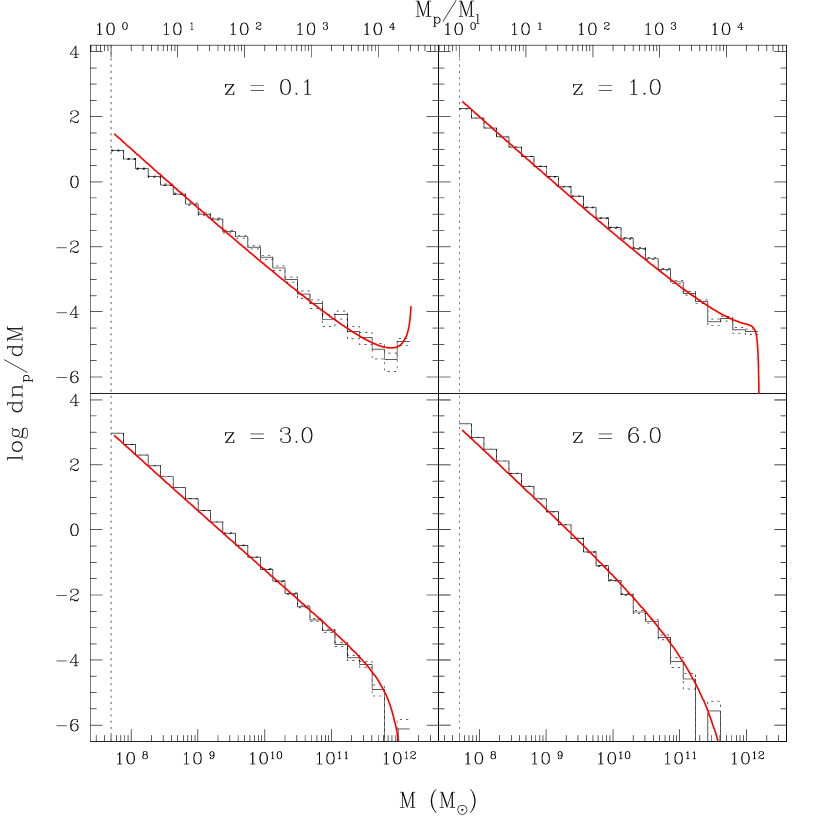
Figure 1: The average number of progenitors in a merger tree as a function of mass (in $M_{\odot}$ along the bottom axis, or in units of the resolution limit $M_{\rm l}$ along the top axis), at four different redshifts (histogram). The dotted histograms show the error in the mean, and the smooth curves show the Press-Schechter predictions.

As a simple test of the global properties of our merger trees, we can calculate the formation epoch of the main halo in each tree, that is the time when the main system had assembled some fraction $f$ of its final mass. The resulting distribution can be calculated analytically in PS theory:

$$P_{f}(z,M_{0})=\int^{S_{f}}_{S_{0}}{{M_{0}}\over{fM_{0}}}f_{S_{1}}(S_{1},\omega_{1}|S_{0},\omega_{0}){\rm d}S_{1}\,,$$ (5)

(LC93, equation 2.26), where $S_{f}=\sigma^{2}(fM_{0})$ and the other variables are as above. Fig. 2 shows the distribution of formation redshifts for the SCDM trees used in this paper, compared to the analytic distribution, for $f=0.9$ , $f=0.75$ and $f=0.5$ (denoted $z_{f,90}$, $z_{f,75}$ and $z_{f,50}$ respectively). There is good agreement with the analytic estimate down to $f=0.5$, where the definition of $z_{f}$ breaks down as a present-day halo of mass $M$ may have more than one progenitor with a mass of $fM$.

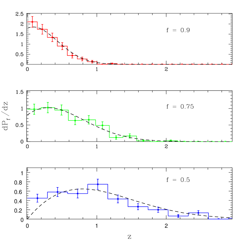
Figure 2: The distribution of formation redshifts for SCDM trees, compared to the analytic prediction, for $f=0.9$, $f=0.75$ and $f=0.5$ (top, middle and bottom panels respectively).

We will show in paper II that many global properties of substructure correlate strongly with the relative age of the halo. It is not clear what value of $f$ to choose when estimating the age of a system. In Fig. 3 we show a comparison between the formation epochs defined for different values of $f$, for individual merger trees. Beyond the limits imposed by the requirement that haloes grow monotonically, i.e. that $z_{f,90}<z_{f,75}<z_{f,50}$ (dashed lines), there is only a slight correlation between the different formation times, with fairly large scatter. We will show in part II that one can distinguish different effects in the spectrum of halo substructure, using the different formation epochs to characterise separate phases in the mass accretion history of a given halo.

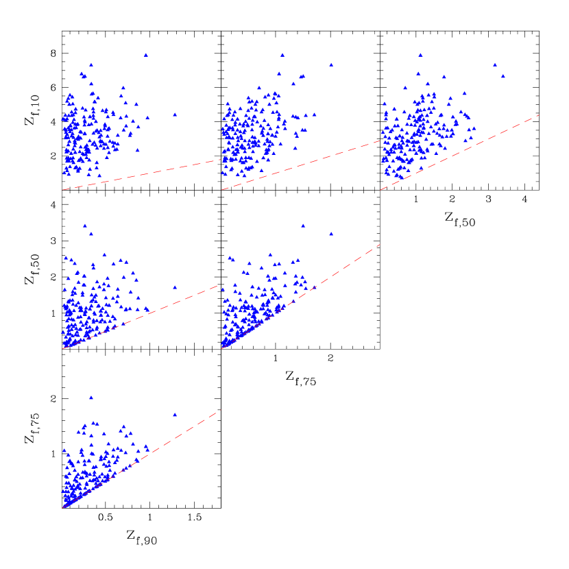
Figure 3: Correlations between the formation epochs defined using different values of $f$. The dashed line shows the region excluded by the requirement that the halo grow monotonically.

2.2 Structural properties of the main system

The spherical collapse model described in section 2.1 also provides an estimate of the final density of the virialised region of a halo. If one assumes that a collapsing density fluctuation virialises through violent relaxation when the formal solution reaches zero radius, and that virialisation conserves the initial energy of the system, then virialisation should occur when the mean density of the system relative to the critical density reaches a specific value $\Delta_{\rm c}\equiv\rho_{\rm vir}/\rho_{\rm c}$. The precise value of $\Delta_{\rm c}$ has been calculated for various CDM cosmologies (e.g. Peebles 1980 or Padmanabhan 1993 for SCDM; Maoz 1990 or LC93 for OCDM; Kochanek 1995 or Eke, Cole & Frenk 1996 for LCDM) and lies in the range 100–200. Although this analytic estimate ignores several complications in the evolution of overdense regions, simulations show that it is approximately correct (Lacey & Cole 1994; Navarro, Frenk and White 1997, 1997, NFW96 and NFW97 hereafter).

In what follows, we will therefore assume that the virial density is exactly $\Delta_{\rm c}\rho_{\rm c}(z)$ at any epoch $z$, so the radius of a halo of mass $M$ at that epoch is simply

$$r_{\rm vir}(z)=\left({{3\,M(z)}\over{4\pi\Delta_{\rm c}\rho_{\rm c}(z)}}\right)^{1/3}\,,$$ (6)

and circular velocity at the virial radius is:

$$V_{\rm c,vir}(z)=\left({{G\,M(z)}\over{r_{\rm vir}(z)}}\right)^{1/2}\,.$$ (7)

We note that in the EPS picture, all haloes seen at a given epoch have the same mean density within their virial radius, independent of mass. We do expect systematic differences in the density distribution within the virial radius for haloes of different masses, however, as discussed below.

2.2.1 The universal density profile

The spherical collapse model does not specify how dark matter behaves interior to the virial radius. One of the most important results of numerical simulations of halo formation was the discovery that the spherically averaged density profile of haloes has a characteristic form which is independent of cosmology (NFW96; NFW97; Moore et al. 1998). In its outer regions, close to the virial radius, this universal density profile has a logarithmic slope of $-3$; the slope then decreases to $-2$ at a characteristic radius near the peak of the rotation curve, and then drops further to a central slope of less than $-2$.

Two analytic forms commonly used to describe the simulation results are the Navarro, Frenk and White (NFW) profile (NFW96; NFW97):

$$\rho(r)={{\rho_{\rm s}\,r_{\rm s}^{3}}\over{r\,(r+r_{\rm s})^{2}}}$$ (8)

and the Moore profile (Moore et al. 1998):

$$\rho(r)={{\rho_{\rm s}\,r_{\rm s}^{3}}\over{r^{1.5}\,(r^{1.5}+r_{\rm s}^{1.5})}}$$ (9)

In their outer regions, these profiles are almost identical if one normalises the scale radius $r_{\rm s}$ and density $\rho_{\rm s}$ such that they match at the radius where the circular velocity peaks, $r_{\rm p}=2.163\,r_{\rm s}({\rm NFW})=1.25\,r_{\rm s}({\rm M})$. A similar, non-analytic profile with a central inner slope of $-0.75$ was described by Taylor & Navarro (2001); it has a scale radius of $r_{\rm s}({\rm TN})=1.67\,r_{\rm s}({\rm NFW})$, and also matches the universal profile in its outer regions if normalised as described above. The precise value of the inner logarithmic slope is still controversial, however, as discussed in the next section.

2.2.2 The central cusp

The slope of the central cusp in haloes is particularly hard to determine from simulations, as it is strongly affected by softening, mass and force resolution. Initially, simulations indicated the central cusp had a logarithmic slope of $-1$ (NFW96, NFW97). Subsequent convergence tests at higher resolution suggested that the slope was steeper, possibly as steep as $-1.5$ (e.g. Moore et al. 1998; Fukushige & Makino 2001). The most recent high-resolution simulations find that while the central slope is less than $-1$, there may be more mass in the central regions of haloes than predicted by the NFW formula (Power et al. 2003). A further complication is that the logarithmic slope may continue to change slowly, not approaching its final value until it is well below the resolution limit of current simulations (Taylor & Navarro 2001). When considering subhalo evolution, the amount of mass in the central regions is generally more important than the exact slope of the density profile, so we will use the analytic Moore profile in our model by default, to account for the extra mass seen by Power et al. (2003). We expect results for the TN profile to be similar, as explained in section 3.4. In paper II we will consider the effect of other density profiles, such as an NFW profile, on our results.

2.2.3 Halo concentration

The one remaining parameter required to specify a halo’s density profile completely is its concentration, defined as $c\equiv r_{\rm vir}/r_{\rm s}$, which measures the position of the break radius relative to the virial radius of the system. Generally low-mass haloes, which form at early times, are more concentrated (i.e. $r_{\rm s}$ is smaller relative to $r_{\rm vir}$) than massive haloes, which form later. It was first suggested that the break in the universal density profile marks the boundary between material built up during the initial formation of the halo or its precursors at early times, and material accreted on to these cores at later times (NFW96, NFW97). There is now some direct confirmation of this picture from simulations (Wechsler et al. 2002; Zhao et al. 2002), and there are several predictions of the concentration of haloes as a function of their mass and the redshift, based on this interpretation (NFW96; Bullock et al. 2001b; Eke Navarro and Steinmetz 2001 – ENS01 hereafter). We will assume the concentrations predicted by the ENS01 model, the most recent fully-analytic model. We calculate ENS01 concentrations using code made publicly available by the authors, and convert these to Moore concentrations using the ratio of scale radii given above, $c_{\rm M}=(1.25/2.163)\,c_{\rm NFW}$. We note that for very massive haloes or at very high redshifts, the ENS code predicts concentrations of less than 1, presumably because these objects are more massive than the typical mass assumed to have collapsed by that redshift. Since the authors do not measure any concentrations below $\simeq$ 1–2 in their analysis of the simulations, we assume $c_{\rm NFW}=1$ is the minimum concentration for a bound halo and ignore concentrations below this. The exact value of the minimum should be unimportant in practice, since almost no haloes in our merger trees have concentrations this low.

We also note that there is both a large scatter in measured halo concentrations relative to the ENS01 predictions or those of other analytic models based on average properties, and that this scatter correlates with the mass accretion histories. The more recent models of Wechsler et al. (2002) and Zhao et al. (2002), may be more accurate in this respect, but they require a detailed knowledge of the mass accretion history, which will not always be available for all the systems in our model. Our assumed halo concentrations may have some effect on our results, particularly the concentration of the central potential in the main system. We will discuss this issue further in paper II.

2.3 Mergers

For an individual halo, the mass $M(z)$ can be calculated as described in section 2.1. In the EPS approach, sudden jumps in this mass accretion history are interpreted as merger events, where one or more distinct virialised haloes join up with the first system. Following these mergers back in time then produces full merger ‘trees’, as discussed previously. The resulting merger histories contain no spatial information about merger events, however. In order to relate individual merger events to infalling subhaloes, we need to examine the EPS definition of a merger in more detail.

2.3.1 Timing and orbital energy

In EPS models, two haloes ‘merge’ when they are both inside a region with a characteristic density $\Delta_{\rm c}\rho_{\rm c}(z)$. This same density characterises the virialised region of an isolated halo. Thus when a small halo of mass $M_{1}$ and virial radius $r_{1}$ merges with a halo of mass $M_{2}>>M_{1}$, the virial radius of the new, combined system will be $r_{1+2}\simeq r_{2}>>r_{1}$, and thus the actual ‘merger’, that is the moment when the volume containing both haloes reaches the density $\Delta_{\rm c}\rho_{\rm c}(z)$, will occur roughly when the smaller halo crosses the virial radius of the larger system for the first time. More generally, even if $M_{1}$ is larger relative to $M_{2}$, the merger will still occur roughly when the infalling halo first crosses a spherical boundary of radius $r_{1+2}=(3(M_{1}+M_{2})/4\pi\Delta_{\rm c}\rho_{\rm c}(z))^{1/3}$ around the main halo. We will take this precise moment as the event recorded in the merger tree. Once this first infall has occurred, we include the mass of the satellite as part of the main system when calculating its potential, since this is the mass assumed in the merger tree at subsequent times. (This introduces a slight inconsistency in our orbital calculations – satellites move in a potential that includes their own mass – but the effect should be minor except for major mergers, which evolve very quickly, and where we do not expect our simplified orbital calculations to be accurate in any case.)

What velocity should one assign to a merging halo? In the spherical collapse model, assuming no shell-crossing (that is assuming the merging halo falls in radially under the influence of a constant mass interior to its radius, and experiences no other forces beyond this), then the velocity of the subhalo when it ‘merges’ will be

$$V_{\rm infall}=V_{\rm c,vir}=\left({{GM_{\rm vir}}\over{r_{\rm vir}}}\right)^{1/2}\,,$$ (10)

where $M_{\rm vir}$ is the mass of the whole system, including the new subhalo, within its virial radius $r_{\rm vir}$. Numerical simulations confirm this prediction; Tormen (1997), for instance, finds an average velocity for merging satellites (in the sense defined above) of $1.1\pm 0.1\ V_{\rm c,vir}$. In what follows we will assume that $V_{\rm infall}=V_{\rm c,vir}$ exactly, for single merger events. (Infalling groups will have an additional scatter in their velocities, as explained in section 5.3.)

2.3.2 Angular momentum

The angular momentum of infalling satellites is harder to estimate, although one can attempt to derive it by tidal torquing arguments (Peebles 1969), or by assuming a density distribution and a background potential (van den Bosch et al. 1999). A convenient parameterisation for this quantity is the circularity of the orbit $\epsilon\equiv L/L_{\rm c}$, the ratio of the (initial) angular momentum $L$ to the angular momentum of a circular orbit with the same energy, $L_{\rm c}$ (LC93). Several high-resolution simulations of individual haloes suggest that $\epsilon$ has a roughly Gaussian distribution between 0 and 1, with a peak at 0.5–0.55 and a dispersion of 0.2–0.3 (Navarro, Frenk & White 1995; Tormen 1997; Ghigna et al. 1998). We note that for major mergers, the lower-resolution but larger-volume simulations of Vitvitska et al. (2002) find larger values of $V_{\rm infall}/V_{\rm c,vir}$ and a more skewed distribution of angular momenta. This is partly because they normalise to the circular velocity of the most massive halo in a pair, however, and this may be substantially smaller than the final circular velocity of the merger remnant in the case of a major merger. Since they only consider a few outputs of their simulation, it is also not clear whether the satellites have been caught on their first infall into the larger system. Thus we will assume the high-resolution results are more indicative of the initial angular momentum distributions of satellites.

In section 3, we will consider satellite evolution for various specific values of $\epsilon$. In section 4 and in our full model, we will use a Gaussian distribution with a mean ${\overline{\epsilon}}=0.4$ and dispersion $\sigma_{\epsilon}=0.26$, which after selective disruption of the more radial orbits gives a mean of ${\overline{\epsilon}}=0.55$ and a variance of $\sigma_{\epsilon}=0.23$ in the surviving satellites, similar to the distribution in Tormen (1997) or Ghigna et al. (1998). In paper II we will also discuss the effect of changing the energy and angular momentum distributions.

2.3.3 Structure of the merging halo

In the EPS model, as noted above, distinct haloes merging at any epoch will have the same average density within their virial radius, independent of mass. Furthermore, they should also obey the concentration relations described in section 2.2.3. Thus, given the epoch of a merger and the mass of the infalling halo from a merger tree, we can also calculate its initial virial radius, scale radius and density profile. This is enough to describe the infalling system completely, neglecting higher-order substructure it may contain. We will consider this final complication next.

2.4 Substructure and self-similarity

From the discussion in the previous section, within our simplified description of structure formation the initial conditions for cosmological mergers between haloes are well defined. Specifically, an individual event within a merger tree corresponds to a halo with a well-defined density profile, on an orbit chosen from a specific distribution, crossing the virial radius of the new, combined system for the first time.

As a halo merges, it will be stripped of its outer regions. The remaining core will be denser than most of the main system it orbits in, and may persist as a distinct subhalo for many orbits. Since the infalling system has itself formed through hierarchical merging, however, it should contain its own dense substructure. This ‘higher-order’ substructure may survive within the main system even after its original parent has been disrupted, just as galaxies merging into a cluster as part of a small group may be stripped from the group, but will continue to survive as distinct objects. Much of this hierarchy will not be resolved in even the largest of current simulations, but it may make an important contribution to halo substructure, as shown in section 5.

This leads to a tricky problem when modelling substructure in hierarchically assembled haloes. The statistical properties of substructure can be determined most accurately by considering the evolution of individual subhaloes in a simplified system. A full description of substructure should really be applied recursively, however, considering the effect of substructure within substructure and so one. Thus the process of developing and testing a model of substructure is necessarily iterative. The model used to include substructure in a merger tree should also be computationally efficient, treating each step of the merging process with only a few calculations, so that it will be able to handle many levels of the merger hierarchy.

To begin with, in the next section we will consider the evolution of subhaloes in a very simple system, in order to establish certain basic patterns. While the density profiles and orbits will be chosen as described above, we will fix the mass, concentration and density of the main system, and give the infalling subhaloes the same density as the main system. Thus, in effect we will be considering the evolution of a system cutoff from hierarchical growth at some point, and left to evolve without any further accretion or change in its structural properties. In section 4, we will then consider the evolution of subhaloes in evolving systems, with model parameters that have been chosen after iterating several times. Finally, in section 5 we will explain how to include this information in merger trees, and how we have adjusted the parameters in our model by iteration.

3 Evolution of substructure in a static system

3.1 Review of previous work

In TB01, we developed a semi-analytic model for the dynamical evolution of spherical satellites in the potential of a larger system. This model includes simple descriptions of the most important physical processes that determine satellite evolution, namely dynamical friction, tidal stripping, and tidal heating. Dynamical friction, the drag force produced as a massive object moves through a background of particles, is modelled using Chandrasekhar’s formula (Chandrasekhar 1943), with the Coulomb logarithms left as free parameters. Tidal stripping is modelled by assuming that material outside the instantaneous tidal radius of the satellite is stripped off on a time-scale equal to the dynamical time of the satellite at its half-mass radius. By introducing this time-scaling, we were able to capture the dependence of mass loss on orbital pericentre and apocentre, which is not reproduced in simpler treatments (Taylor 2001). Finally, to model the rapid shocks experience by the satellite when it passes through the pericentre of its orbit or through the plane of a galactic disk, we include a heating term in the expression for mass loss, with an adjustable heating coefficient.

Overall, the model in TB01 thus predicts orbital evolution and mass loss for satellites using three free parameters; a Coulomb logarithm $\Lambda_{\rm s}$ for the halo and other spherically distributed material, a Coulomb logarithm $\Lambda_{\rm d}$ for the galactic disk, and a heating coefficient $\epsilon_{\rm h}$. Comparing model predictions to a set of 15 high-resolution simulations of encounters between satellites and disk galaxies by Velázquez and White (1999), we found we were able to reproduce the orbital evolution and mass-loss history of the satellites to within 10–20 per cent over most of their evolution (until they had lost $\simeq 90$ per cent of their mass), using as single set of parameters, $\Lambda_{\rm s}=2.4$, $\Lambda_{\rm d}=0.5$ and $\epsilon_{\rm h}=3.0$. The latter value of the heating coefficient also produces quite a good fit to the mass-loss rates measured in a set of high-resolution simulations by Hayashi & Navarro (Hayashi et al. in preparation; see Taylor 2001 for a comparison), which use very different potentials, orbits and density profiles, so we have reason to believe it is generally applicable.

TB01 did not discuss the internal structural evolution of satellites. In subsequent work by Hayashi et al. (2003), the evolution of the density profile was found to depend on the total mass loss alone, rather than on the details of the mass-loss history. This paper provides formulae for determining the density profile and characteristic radii of a satellite at any point in its evolution, as well as an estimate of when repeated mass loss will disrupt an object completely.

Taken together, these results constitute a full analytic description of the dynamical evolution of satellites in realistic potentials, and one that is easily applicable to a large number of objects with minimal computational effort, as uses only the global properties of satellites, such as their total mass and the characteristic radii of their density profile. We will now apply this analytic description to the problem of subhalo evolution. We take the same values for the dynamical parameters, $\Lambda_{\rm s}=2.4$ and $\epsilon_{\rm h}=3.0$, determined in TB01, and scale $\Lambda$ by $(M_{\rm sat}/M_{\rm halo})^{-1}$ (where $M_{\rm sat}$ is the mass of the satellite and $M_{\rm halo}$ is the mass of the main system), as discussed in section 4.1 of TB01. There is no need to specify $\Lambda_{\rm d}$, since the potentials considered in this paper have no disk component.

3.2 The orbital time-scale

First, we will examine the basic properties of the orbits specified in section 2.3, that is orbits starting at the virial radius of a large halo with a Moore density profile, with a total initial velocity of magnitude $V_{\rm c}$ and various possible circularities. We choose a concentration of $c_{\rm M}=10$ for the main system, the value predicted by the ENS01 concentration relations for a halo similar to that of the Milky Way, at $z=0$ in our SCDM cosmology. Our fiducial system has a mass of $1.6\times 10^{12}{\rm M}_{\odot}$ and a virial radius of 314 kpc, but our results scale in a straightforward way and can all be described in terms of scaled variables. Given this scaling, the evolution of a satellite subhalo in our model will depend only on its mass relative to the mass of the main system, its concentration, the initial circularity of its orbit, and the concentration of the main system. In most of this section we will also ignore dynamical friction, to simplify the analysis of the dynamics. Thus for a given main potential, the evolution of a satellite will depend only on its initial concentration and its circularity.

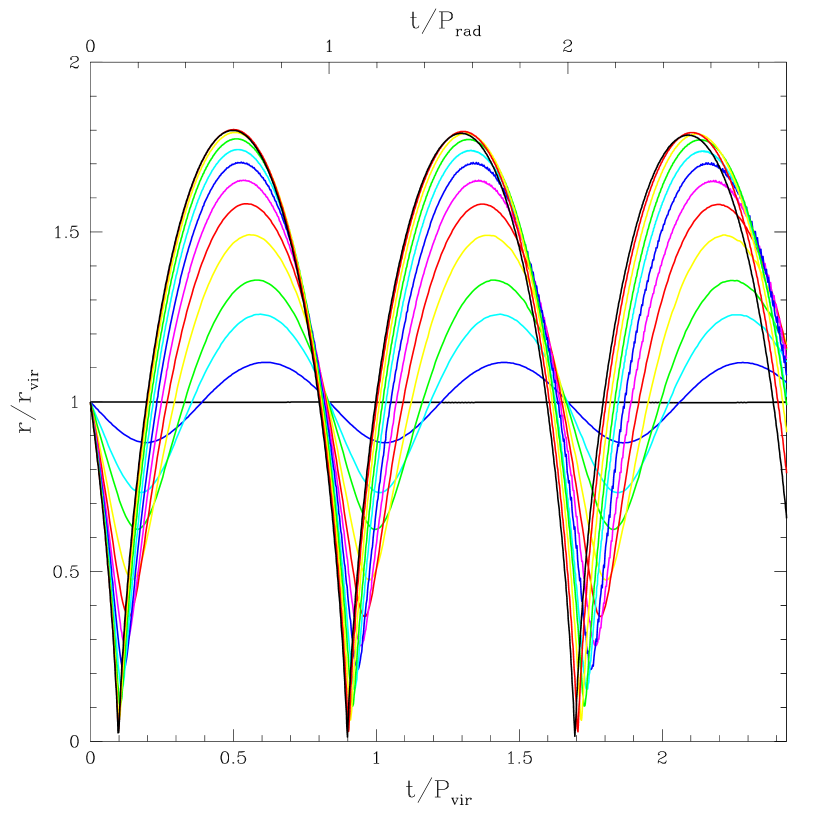
Figure 4: Radius (in units of the virial radius) versus time (in units of the azimuthal period of a circular orbit at the virial radius, $P_{\rm vir}=2\pi\,r_{\rm vir}/V_{\rm c,vir}$ ), for orbits of circularity $\epsilon=$ 1.0, 0.99, 0.95, 0.9, 0.8, 0.7, 0.6, 0.5, 0.4, 0.3, 0.2, 0.1, and 0.05. The top axis shows time in units of the period for small radial oscillations $P_{\rm rad}=2\pi/\kappa$ (see text). Dynamical friction has not been included.

We will see in the section 3.3 that mass loss occurs primarily at the pericentric passages in a subhalo’s orbit. Thus the characteristic time-scale for the evolution of substructure will be the period of radial oscillations (or ‘radial period’). Fig. 4 shows the radial coordinate of satellites on orbits of various different circularities, ranging from $\epsilon=$ 0.05 to $\epsilon=$ 1.0 (different curves), with the vertical axis scaled by the virial radius of the main system and the horizontal axis scaled by the (azimuthal) period of a circular orbit at the virial radius, $P_{\rm vir}=2\pi r_{\rm vir}/V_{\rm c,vir}$. (The latter quantity is equal to $H_{0}^{-1}\,(8\pi^{2}/\Delta_{\rm c})^{1/2}$ from the spherical collapse model; for the SCDM cosmology considered here $\Delta_{\rm c}=18\pi^{2}$, and thus $P_{\rm vir}=2/3\,H_{0}^{-1}$ is simply the age of the universe at the epoch which characterises the virial density of the main system.) Dynamical friction has been ignored, as mentioned earlier, so the orbits shown in Fig. 4 correspond to those of low-mass satellites.

The variation in radius is regular and periodic, but clearly the period differs from $P_{\rm vir}$. In fact, it is roughly equal to the period for small radial oscillations at the virial radius, $P_{\rm rad}\equiv 2\pi/\kappa$, where $\kappa$ is the epicyclic frequency:

$$\kappa={{V_{\rm c}}\over{r_{\rm vir}}}\left(1+{{{\rm d}\ln M}\over{{\rm d}\ln r}}\right)^{1/2}\,,$$ (11)

as expected from orbital theory for a spherical system with mass $M$ interior to $r$ (Binney and Tremaine 1987, section 3.2.3). This quantity will vary with the slope of the density profile. Fig. 5 shows the logarithmic slope (top panel) and the ratio of the radial and azimuthal periods (bottom panel) at the virial radius as a function of the concentration of the system, for haloes with NFW (solid) or Moore (dashed) profiles. For Moore profiles with concentrations typical of galaxy haloes, $P_{\rm rad}\simeq 0.835\pm 0.015\,P_{\rm vir}\simeq 5.24(r_{\rm vir}/V_{\rm c,vir})$. Strictly speaking, this radial period should apply only to small amplitude oscillations about a circular orbit, but from Fig. 4 we can see that it describes the period of radial oscillations reasonably well even for extremely non-circular orbits. There is a slight change in the radial period with orbital circularity – the oscillations in radial orbits are about 5 per cent faster than those in almost circular orbits – but the main difference is a shift of the time of pericentric passage within an orbit from 0.125 $P_{\rm rad}$ to 0.25 $P_{\rm rad}$ as $\epsilon$ increases. In what follows, we will assume $P_{\rm rad}$ is the basic period for subhalo orbits, and that pericentric passages occur somewhere between 1/8 and 1/4 of a radial period, and then periodically thereafter.

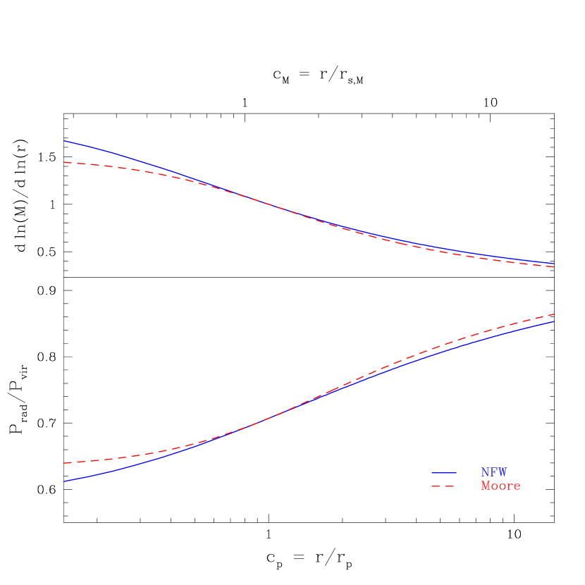
Figure 5: The logarithmic derivative of the mass profile (top panel) and the radial period at the virial radius $P_{\rm rad}$ (bottom panel) versus concentration, for NFW and Moore profiles (solid and dashed lines respectively).

Finally, although we have calculated orbits in the potential generated by a Moore density profile, we note that all but the most radial orbits would be very similar in an NFW profile (of if we had added a small galactic component to the potential) since most orbits do not enter into the central regions of the potential where the profiles differ (e.g. in Fig. 4, only orbits with $\epsilon<0.2$ reach radii of less than $0.1\,r_{\rm vir}$). We also note that the extremely radial orbits plotted in this section require very small time-steps to integrate properly. For realistic distributions of orbital circularity, few subhalo orbits are this expected to be this radial, as discussed below. Since the mass-loss model developed in TB01 is unlikely to be accurate for orbits with very small pericentres in any case, in our full model we will consider subhaloes disrupted when they come very close to the centre of the main system ($r<0.01\,r_{\rm vir}$), and stop following their orbital evolution at that point. Otherwise, subhalo orbits are calculated with an adaptive time-step, sufficiently small to provide reasonable accuracy given this cutoff at very small radii.

3.3 Mass loss

We proceed to consider mass loss on typical orbits. From the previous discussion, the mean density of haloes (within their virial radius) when they merge will be the same as the mean density of the main system, and their initial mass will be specified by the merger tree. If we fix the density profile and concentration of the main system, assume the subhalo has a Moore density profile, and ignore dynamical friction, then the evolution of a subhalo will depend only on its concentration and on the circularity of its orbit. In this section we will study the case $c_{\rm M}$ (sat) $=c_{\rm M}$ (main) $=10$; we will then show results for a typical range of concentrations below. We include the effects of tidal shocks, as in TB01, but choose parameters appropriate to slow shocks (an adiabatic coefficient $\gamma=1.5$ and a shock criterion $t_{\rm shock}<4\,t_{\rm orb,sat}$; see Gnedin & Ostriker (1999) or TB01 for an explanation of these parameters), since the passage through pericentre is slower than the passage through a disk considered in TB01.

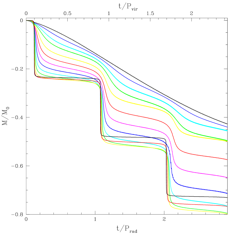
Figure 6: Bound mass fraction versus time, in units of the radial period $P_{\rm rad}$ (bottom axis) or the azimuthal period $P_{\rm vir}$ (top axis). The curves are for the same circularities as in Fig. 4, and dynamical friction has not been included, as before.

Fig. 6 shows the fraction of the subhalo’s original mass that remains bound as a function of time, for the same set of orbits plotted in Fig. 4. We have estimated the bound mass using the model from TB01, which assumes that a fraction $\Delta t/t_{\rm d,h}$ of the mass outside the instantaneous tidal radius is lost in a time step of length $\Delta t$ (where $t_{\rm d,h}$ is the dynamical time of the system at its half-mass radius), and also includes a heating term to correct for rapid tidal shocking. This model reproduces the pattern of continuous mass loss throughout the orbit, with a sharp increase at each pericentric passage, that has been seen in simulations of tidal stripping and heating. For the most radial orbits, almost all the mass loss occurs at pericentre, while for circular orbits mass loss is slower but continuous. In general, satellites on more radial orbits lose more mass, mainly because they pass through smaller pericentres and experience stronger tidal fields. This trend is not completely monotonic, however, since a satellite on an extremely radial orbit spends very little time close to the pericentre of its orbit, where tides are strongest. Comparing the most extreme curve in Fig. 6 to slightly less radial orbits, we see that while the mass loss at the first pericentric passage is similar, less mass is lost immediately afterwards, as the satellite moves away from the pericentre of its orbit faster than it would if its orbit were more circular.

Fig. 7 shows the fraction of the original mass which remains bound after one radial period, as a function of orbital circularity. The general trend towards more mass loss on radial orbits is clear, but orbits with $\epsilon\simeq 0.2$–0.3 produce the most net mass loss per radial period. A rough fit to the bound mass fraction after one radial period as a function of circularity, $M/M_{0}\simeq 0.35\,\epsilon^{2}+0.2\,\epsilon+0.58$, is also shown.

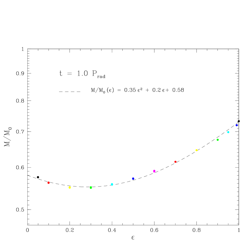
Figure 7: Bound mass fraction after one radial period ($t=1.0\,P_{\rm rad}\simeq 5.24\,r_{\rm vir}/V_{\rm c}$), as a function of circularity $\epsilon$, for subhaloes with a Moore density profile of concentration $c_{\rm M}=10$ and no dynamical friction. The dashed curve shows the functional fit $M/M_{0}=0.35\,\epsilon^{2}+0.2\,\epsilon+0.58$.

The scaling of mass loss with orbital and halo properties is particularly important for haloes with cosmological profiles, that is profiles with a central region that is sub-isothermal. Within some radius, the total energy of these systems is actually positive, as there is insufficient mass to bind the material in the core (Hayashi et al. 2003). Thus repeated mass loss may disrupt such systems completely if they cannot readjust themselves into a new virial equilibrium quickly enough. We discuss this point in more detail in the next section.

3.4 Disruption

3.4.1 The disruption criterion

One important question regarding the evolution of substructure is whether it can ever be fully disrupted by tidal forces, and if so when this occurs. This point is very hard to resolve using N-body simulations alone, since subhaloes become more and more sensitive to purely numerical effects as they lose mass. One basic analytic approach to determining the stability of a system is to calculate its net kinetic and potential energy interior to some radius (calculated as if the system were truncated at that radius), prior to any heating or stripping:

$$E(<r) = K(<r)+W(<r)$$ (12)

$$= \int_{0}^{r}\rho(r^{\prime})\,\overline{v^{2}}(r^{\prime})\,2\pi\,r^{\prime 2}{\rm d}r^{\prime}$$

$$+ \int_{0}^{r}\rho(r^{\prime})\,\phi(r^{\prime},r)\,2\pi\,r^{\prime 2}{\rm d}r^{\prime}\,,$$

where $\overline{v^{2}}(r^{\prime})$ is the velocity dispersion at $r^{\prime}$ and $\phi(r^{\prime},r)$ is the potential at $r^{\prime}$ generated by material within $r$. If tidal stripping removes material from the outer part of a system without affecting the distribution function of the remaining material too much, then the system should be unstable once it is stripped to a radius $r_{\rm bind}$ within which the total energy, as defined above, is positive.

For a given density profile, we can calculate the initial critical radius using equation (12). For an NFW profile, $r_{\rm bind}=0.77\,r_{\rm s}\,({\rm or}\ 0.353\,r_{\rm p})$, for a TN profile $r_{\rm bind}=0.399\,r_{\rm s}\,({\rm or}\ 0.307\,r_{\rm p})$, and for a Moore profile $r_{\rm bind}=0.37\,r_{\rm s}\,({\rm or}\ 0.296\,r_{\rm p})$, while for an isothermal profile the critical radius is infinite, since the total energy, as defined above, is negative at all radii.

This stability criterion has the important consequence that systems with sub-isothermal cusps or cores will become unstable and disrupt rapidly once they have lost a large fraction of their mass. In fact, in the most recent and most detailed numerical study of mass loss (Hayashi et al. 2003), it was found that systems on circular orbits disrupt if their tidal radius $r_{\rm t}$ is less than $2\,r_{\rm bind}$. Unfortunately, for general orbits the criterion is not straightforward to apply, since $r_{\rm t}$ varies with time and $r_{\rm bind}$ also varies as the density profile and distribution function change due to mass loss. If we assume that a system re-virialises instantaneously whenever it loses mass, for instance, then the scaling formula for the stripped density profile proposed in Hayashi et al. (2003) (equations 8–10) predicts that a halo with an NFW profile of concentration $c_{\rm NFW}=10$ will never be disrupted by mass loss, as its total mass will always exceed the mass inside $2\,r_{\rm bind}$. Nonetheless, these formulae do predict a point of minimum stability (in the sense that the tidal radius of the system is close to $2\,r_{\rm bind}$) when the system has lost approximately 97 per cent of its original mass, and $r_{\rm bind}$ is half the original critical radius $r_{\rm bind,0}$. Empirically, Hayashi et al. trace the evolution of systems on radial orbits down to about this level, while for circular orbits they show some systems still bound when they have lost all but $0.3$ per cent or more of their mass, corresponding to a critical radius of roughly $0.1$ of the original.

In what follows, we will parameterise the uncertainty in the disruption criterion by assuming that systems disrupt when $r_{\rm t}<f_{\rm dis}\,r_{\rm bind,0}$, or $M<M_{\rm bind}\equiv M(<f_{\rm dis}\,r_{\rm bind,0})$. Motivated by the simulations, we will consider results for $f_{\rm dis}=0.5$ (‘model A’) and $f_{\rm dis}=0.1$ (’model B’). We will show, particularly in paper II, that our main results do not depend strongly on $f_{\rm dis}$, provided it is in this range or smaller. We also note that in self-consistent simulations of halo formation, few subhaloes will be resolved with sufficiently many particles to trace their survival down to these levels, so we should not be surprised if they resemble our model results for larger values of $f_{\rm dis}$. The fraction of the original mass within $f_{\rm dis}\,r_{\rm bind,0}$ will of course depend on the initial concentration of the system; this dependence is shown in Fig. 8 for the NFW profile, the Moore profile and the TN profile, for $f_{\rm dis}=2.0$, $f_{\rm dis}=0.5$, and $f_{\rm dis}=0.1$.

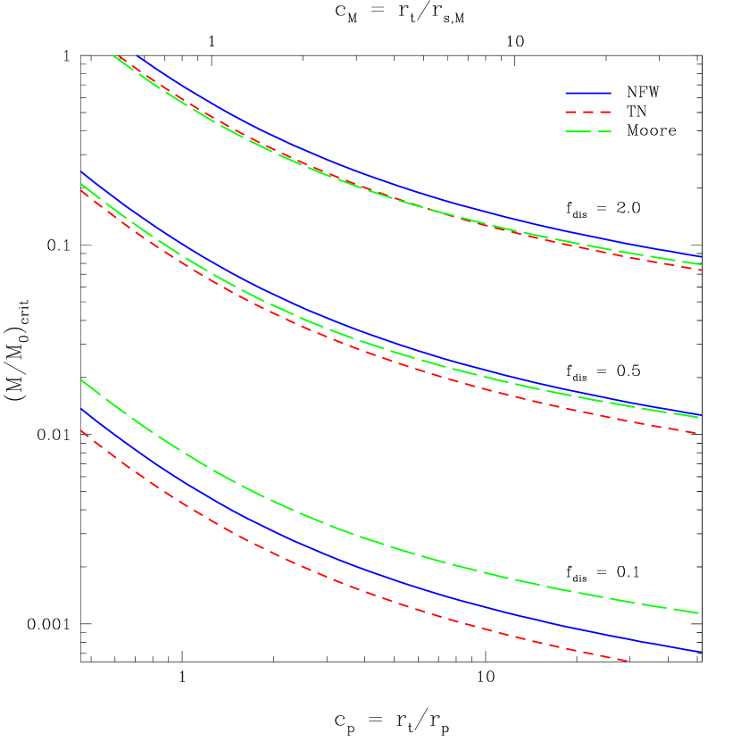
Figure 8: The mass below which a system of a given concentration will be disrupted, as a fraction of its original mass, for disruption parameters $f_{\rm dis}=2.0$, $f_{\rm dis}=0.5$, and $f_{\rm dis}=0.1$. The solid line is for an NFW profile, the short-dashed line is for a TN profile and the long-dashed line is for a Moore profile. The concentration is expressed in terms of the peak radius on the bottom axis, or the equivalent Moore concentration on the top axis.

3.4.2 Implications

In most previous semi-analytic treatments of subhalo evolution, dynamical friction was assumed to be the main process responsible for the destruction of substructure. For the orbits considered here, the time-scale for this process to occur is:

$$t_{\rm dis}=1.2\,e\,{{(M_{\rm h}/M_{\rm s})}\over{\ln(M_{\rm h}/M_{\rm s})}}\,\epsilon^{0.4}\,{P_{\rm vir}\over{2\,\pi}}\,,$$ (13)

(Colpi, Mayer and Governato 1999), where $M_{\rm h}$ is the mass of the main halo, $M_{\rm s}$ is the initial mass of the subhalo, and $\epsilon$ is the initial circularity of the satellite’s orbit. The factor $e>1$ in this formula corrects for mass loss, which in this picture increases the disruption time, by reducing the mass of the satellite and thus the dynamical friction it experiences. As pointed out by Taffoni et al. (2002), since $P_{\rm vir}$ is comparable to the Hubble time, this infall time will be extremely long (hundreds or thousands of Hubble times) for all but the most massive satellites. On the other hand, we saw above that a typical satellite will be stripped of 25–45 per cent of its mass after each orbital period, and that for many systems, this repeated mass loss may eventually result in their complete disruption.

Fig. 9 shows the disruption times, that is the times after which systems have been stripped down to $M_{\rm bind}=M(<f_{\rm dis}\,r_{\rm bind,0})$, in a potential with a Moore profile of concentration $c_{\rm M}=10$, for satellites of concentration 4, 8 or 12 (different point types), on a representative distribution of orbits (see section 2.3) and including dynamical friction, for $f_{\rm dis}=0.5$ (model ‘A’, top panel) and $f_{\rm dis}=0.1$ (model ‘B’, bottom panel). The smooth curves indicate the orbital decay time calculated from equation (13), for $e=1$ (solid lines) and $e=3$ (dashed lines).

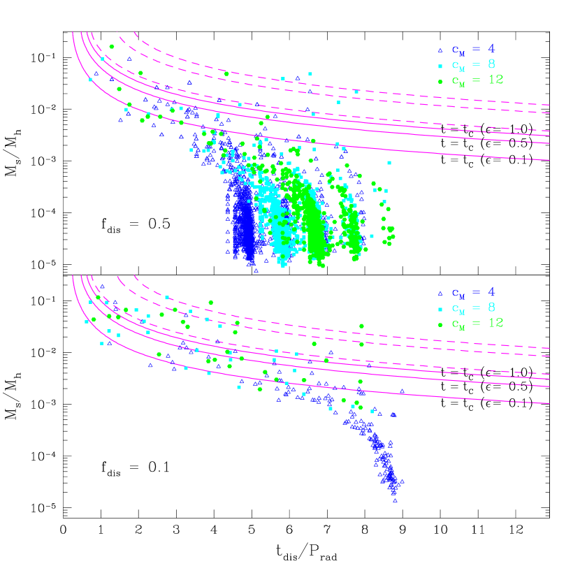
Figure 9: Disruption times for satellites on a distribution of orbits, in static halo with a Moore density profile of concentration $c_{\rm M}=10$, including dynamical friction. The point types indicate the concentration of the satellites. The smooth curves indicate the orbital decay time, as estimated from equation (13), for $e=1$ (solid lines) and $e=3$ (dashed lines), and $\epsilon=1.0$, 0.5 and 0.1 (from top to bottom). The top panel shows results for $f_{\rm dis}=0.5$; the bottom panel shows results for $f_{\rm dis}=0.1$. Note that there are no satellites in these trees that have merged more than 9 radial periods previously, so we cannot measure disruption rates beyond $t_{\rm dis}/P_{\rm Rad}=9$.

We see that while the disruption time scales with mass and is comparable to the orbital decay time for the most massive systems ($M_{\rm s}/M_{\rm h}\ga 0.01$), for less massive systems it becomes roughly independent of mass. In model ‘A’ (top panel), most low-mass systems are disrupted due to repeated mass loss after 5–8 pericentric passages, depending on their concentration, as expected from the mass-loss rates and critical mass fractions given above. Note that there are no satellites in these trees that have merged more than 9 radial periods previously, so we cannot measure disruption rates beyond $t_{\rm dis}/P_{\rm Rad}=9$. From the results in the top panel, however, we expect systems to disrupt after 9–12 orbits in model ‘B’ (bottom panel). We conclude that while the dynamical friction time derived by Colpi et al. (1999) is quite accurate for massive satellites, with $e\simeq 2$, a proper description of mass loss and disruption is essential to determining the evolution of less massive substructure.

3.5 Summary

In this section, we have considered the evolution of subhaloes in the static potential generated by a larger system. We have chosen density profiles and orbital parameters which should be representative of the halo mergers that occur in hierarchical structure formation, and which therefore provide a well-defined set of initial conditions for studying the dynamics of halo substructure. We find that most mass loss occurs as a subhalo passes through the pericentre of its orbit, particularly for the radial orbits typical in cosmological settings. In general, we predict that subhaloes should lose about 25–45 per cent of their mass for each pericentric passage, with the amount of mass loss tending to increase as the orbit becomes more radial. After a number of pericentric passages, this repeated mass loss may lead to complete disruption, although further simulations are required to confirm exactly when this takes place. In TB01 we also found that dynamical friction is also strongest close to the pericentre of the orbit. Thus the overall dynamical state of a subhalo will depend principally on the number of pericentric passages, or the number of orbits (in the sense of radial oscillations), that it has spent in its parent halo. In a static halo, this is simply $n_{\rm o}=\Delta\,t/P_{\rm rad}$, where $\Delta\,t$ is the time elapsed since the satellite first crossed the virial radius of the parent and $P_{\rm rad}$ is the (fixed) radial period defined above.

In a cosmological setting, the radial period of an orbit will vary if the mean density within the orbit changes. In particular, the radial period at the virial radius will increase roughly proportionally to time, as the density inside the virial radius decreases, and even orbits in the inner parts of a halo may develop longer periods if major mergers rearrange material in the halo sufficiently to reduce its mean central density. Subhaloes merging into the main system will have concentrations and densities that depend on their merger epoch. Furthermore, they may also contribute their own substructure, which has already experienced mass loss in earlier stages of the merging hierarchy, to the main system. Thus some of the patterns seen in this section may be obscured in more general situations. In the next section we will consider subhalo evolution in a realistic system, that includes all of these effects. We will show in particular that satellite properties still correlate strongly with $\Delta\,t/P_{\rm rad}$, provided we use the radial period at the time when the satellite first crossed the virial radius to estimate how many times it has orbited within the larger system.

4 Evolution of substructure in a realistic system

To study the evolution of substructure in a realistic halo, we have to take into account the changing mass and structural properties of the main system, as well as any previous evolution of its subcomponents at earlier stages of the hierarchical merging process. The changing properties of the main system can be derived using the semi-analytic methods described in sections 2.1–2.2. Specifically, we can generate a set of representative mass accretion histories, that is functions $M(z)$, for haloes with a given mass at the present day, using extended Press-Schechter methods, and pick one of these to represent the main system. The spherical collapse model then gives us the virial radius $r_{\rm vir}$ and circular velocity $V_{\rm c}$ of the main system at each redshift, while the ENS01 relations give us its concentration $c$ and thus its scale radius $r_{\rm s}$.

The spectrum of infalling satellites is provided by the merger tree, and their initial structural properties can be specified in the same way as for the main halo, as described previously. Higher-order substructure, that is the substructure within infalling objects, is more complicated to deal with. This substructure may lose mass and be disrupted in a smaller parent halo higher up the merger tree before it ever reaches the main system, complicating the picture considerably. Our strategy, as explained in the introduction, will be to develop a simplified description of the evolution of systems in the main halo, and then apply this to the side-branches of the merger tree, adjusting the model parameters iteratively to achieve a consistent solution that predicts the same evolution in the main branch as is assumed in generating the underlying merger tree. In what follows, we will show results for merger trees where we have already performed this iteration, so the adopted parameters are self-consistent; the process required to achieve this convergence will be explained in section 5.

4.1 Orbital evolution

Since period of radial oscillations at the virial radius of the main halo, $P_{\rm rad}$, changes with time as it grows, we will consider the evolution of satellites within this system in terms of $P_{\rm rad}(z_{\rm m})$, the radial period the main halo at the time they first crossed its virial radius. Specifically, if a satellite merges at $z_{\rm m}$ and then spends an interval of time $\Delta t$ in the main halo, we will use $\Delta t/P_{\rm rad}(z_{\rm m})$ as an estimate of the number of radial oscillations it has undergone. This should be reasonably accurate until the mean density interior to its orbit changes, as may happen in a major merger. For brevity, we will write this quantity as $\Delta t/P_{\rm rad}$ in what follows, $P_{\rm rad}$ implicitly being measured at $z_{\rm m}$.

Because we are assuming that the initial orbital energy of infalling satellites depends only on the epoch at which they merge, and the mass of the main halo at this time, we expect the radial coordinate of satellites to show strong correlations with $\Delta\,t/P_{\rm rad}$. Fig. 10 shows the radius and orbital energy of satellites from many different merger trees, plotted as a function of $\Delta\,t/P_{\rm rad}$. (For clarity, we have only plotted one randomly chosen member of every dynamical group – see section 5.3). In the top panel, we see that satellites with recent merger times are close to the virial radius, while successively older systems have reached the pericentre of their orbits, are moving back out to apocentre, or are on their second or third orbit. In general, old systems are concentrated at smaller radii than recently accreted ones (in fact the scatter in orbital apocentre for the older systems is due mainly to the velocity dispersion given to dynamical groups, as discussed in section 5.3). The strong correlation between radius and merger epoch should produce patterns in substructure that are easily visible as coherent clumps or shells in individual haloes. We will discuss the grouping of substructure further in section 5.3 and in paper II.

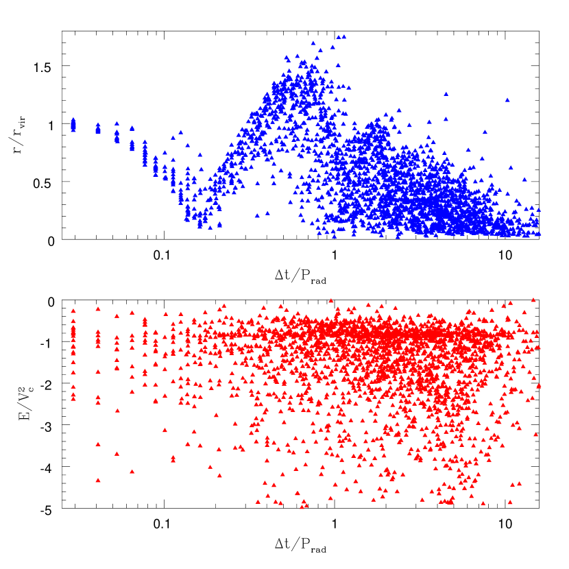
Figure 10: (Top panel) Radial positions of the satellites from a large set of trees, evolved with model A ($f_{\rm dis}=0.5$), versus $\Delta\,t/P_{\rm rad}$. For clarity only one randomly chosen member of every dynamical group has been plotted. (Bottom panel) Orbital energy of the same objects, in units of the present-day circular velocity of the main halo squared, as a function of $\Delta\,t/P_{\rm rad}$.

There is also a slight correlation between $\Delta\,t/P_{\rm rad}$ and the orbital energies of satellites. As the bottom panel in Fig. 10 shows, the mean orbital energy decreases slightly with increasing $\Delta\,t/P_{\rm rad}$, indicating that the oldest satellites within a halo are somewhat more bound than those that have merged more recently. We note, however, that this trend depends on the disruption criterion assumed. We will discuss the effects of disruption on the orbital energy distribution of substructure in detail in paper II.

In summary, since the orbits of recently accreted satellites are both more radially extended and less tightly bound, we conclude that these satellites will be the first to be stripped out of groups when they fall into larger haloes (ignoring for the moment the effects of dynamical friction on the most massive satellites). In the pruning model discussed in section 5, we will therefore use the quantity $\Delta\,t/P_{\rm rad}$ to distinguish between subhaloes that remain associated with their parent system, and those that are stripped off, and should thus treated independently in the next level of the merger hierarchy.

4.2 Mass loss

Given the results of section 3, the average amount of mass loss for subhaloes should also depend strongly on $\Delta\,t/P_{\rm rad}$. Fig. 11 shows the bound mass fraction of individual satellites, that is their bound mass as a fraction of its value at the time of infall into the main system, versus $\Delta\,t/P_{\rm rad}$, for model A ($f_{\rm dis}=0.5$ – filled circles) and model B ($f_{\rm dis}=0.1$ – open squares). For clarity we have only plotted one satellite per dynamical group, as in Fig. 10. The lines indicate the approximate time of successive pericentric passages. We see that the pattern evident in Fig. 6 is reproduced, although with more scatter and greater mass loss in some cases, due to the different orbits and concentrations considered and the effects of dynamical friction on the pericentric radius. Overall, the average bound mass fraction decreases for the first five or six radial periods, but increases slightly thereafter, as the only systems surviving at this point have relatively circular orbits or are more concentrated, raising the average.

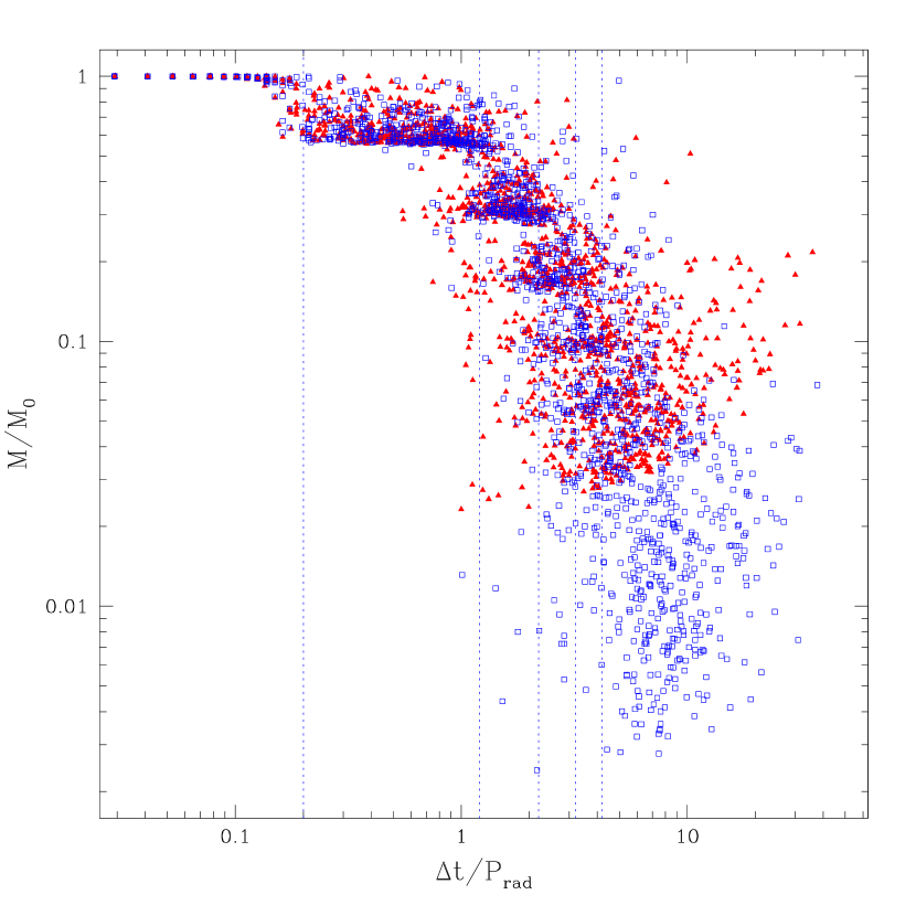
Figure 11: The mass of individual satellites, as a fraction of their mass at the time of infall, versus $\Delta\,t/P_{\rm rad}$. Filled triangles are for model A ($f_{\rm dis}=0.5$), and open squares are for model B ($f_{\rm dis}=0.1$). The vertical lines indicate the approximate time of successive pericentric passages.

4.3 Disruption

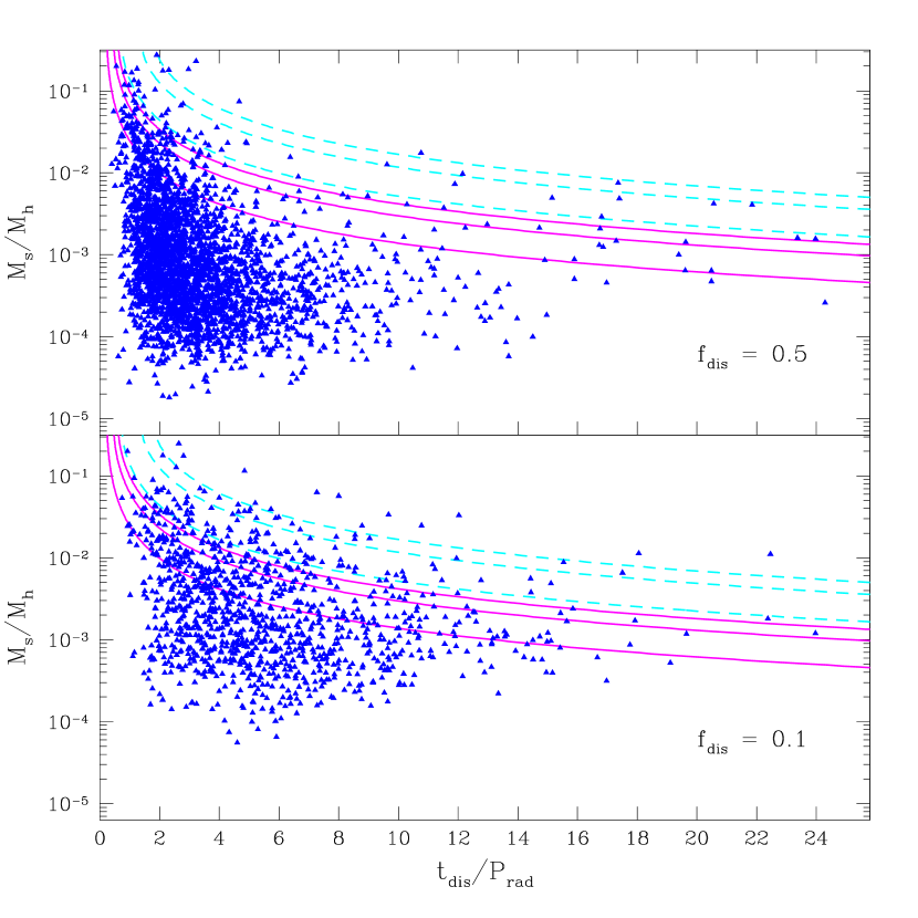
Figure 12: As Fig. 9, but in realistic systems. The top panel shows the disruption time in units of the radial period at the time when the satellite first merges, for model A ($f_{\rm dis}=0.5$); the bottom plot shows the disruption times for model B ($f_{\rm dis}=0.1$). The curves show the orbital decay time for $e=1$ (solid) and $e=3$ (dashed), and for $\epsilon=1.0$, 0.5 and 0.1, as in Fig. 9.

Fig. 12 shows disruption times for subhaloes in a realistic halo, where $P_{\rm rad}$ changes with the virial density, that is roughly proportionally to $t$, and many of the infalling haloes are higher-order, that is to say they have already merged with earlier systems before their final merger with the main halo considered here. (We correct for mass loss due to this previous evolution self-consistently, as explained in section 5.2.) The lines show the estimated orbital decay time, as in Fig. 9. We see that for a realistic halo, disruption times show more scatter and the grouping at specific pericentric passages seen in Fig. 9 is obscured. On average, however, systems are disrupted earlier than in the static case, after $\simeq$ 1–8 pericentric passages for model A ($f_{\rm dis}=0.5$), or $\simeq$ 2–15 pericentric passages for model B ($f_{\rm dis}=0.1$). This is due to prior mass loss in earlier stages of the hierarchical merging process, which reduces the effective concentration of satellites, destabilising them.

Fig. 13 shows the fraction of systems which have survived disruption, as a function of $\Delta\,t/P_{\rm rad}$. For model A ($f_{\rm dis}=0.5$), the disruption probability reaches 50 per cent after 8 pericentric passages, while for model B ($f_{\rm dis}=0.1$), the disruption probability reaches 50 per cent after roughly 15 pericentric passages.

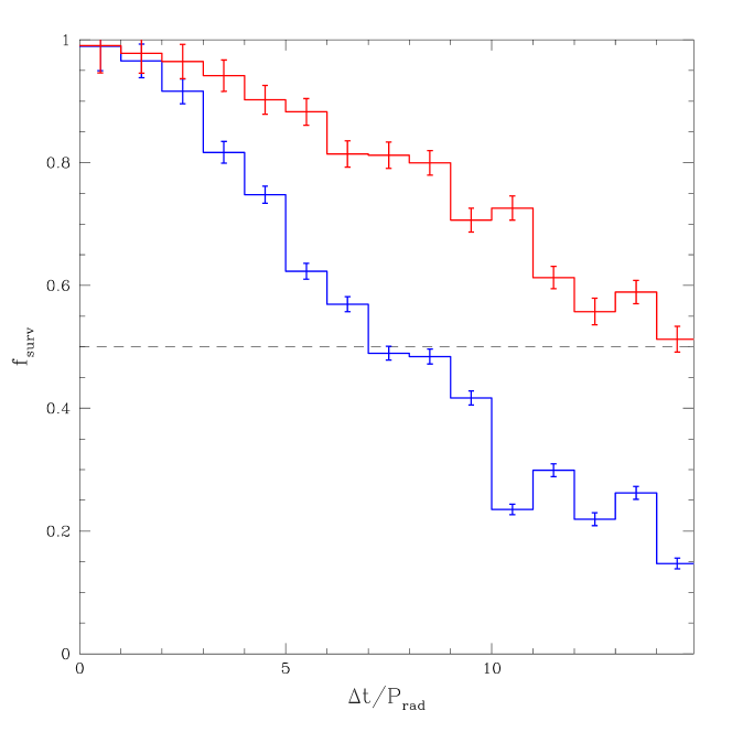
Figure 13: The fraction of the subhaloes that have survived disruption, as a function of the number of radial periods they have spent in the main system. The lower histogram is for model A and the upper histogram is for model B.

So far we have not discussed the dependence of the disruption time on orbital circularity. Generally, disruption occurs sooner for more radial orbits, especially for the most extreme radial orbits. Fig. 14 shows the distributions of initial circularity $\epsilon$ for surviving and disrupted satellites, in a set of trees evolved with model A ($f_{\rm dis}=0.5$). In addition, we plot satellites that have ‘fallen in’, that is objects whose orbits have taken them to pericentres we cannot resolve, below 1 per cent of $r_{\rm vir}$. (Naturally, these systems are on very radial orbits.) Since we cannot follow their subsequent evolution with any accuracy, we take them to be disrupted, as mentioned in section 3.2. Apart from this, there is also a clear shift between the surviving and disrupted distributions. In the bottom panel, we show the fraction of satellites surviving as a function of their initial circularity.

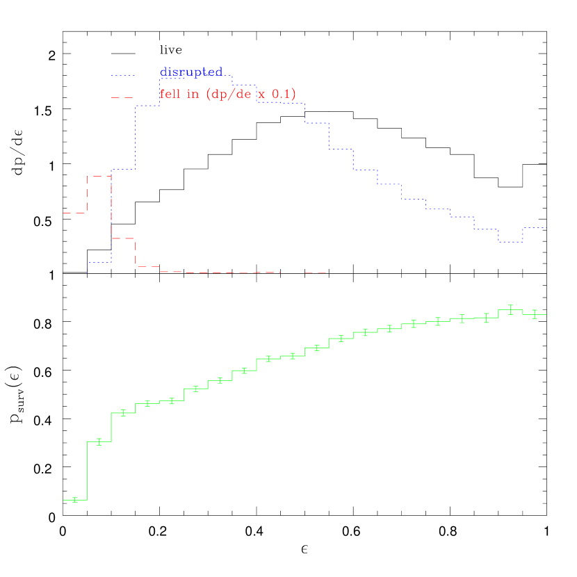
Figure 14: (Top panel) the circularity distributions of surviving and disrupted satellites, as well as those that have fallen in, for model A ($f_{\rm dis}=0.5$). (Bottom panel) the fraction of satellites surviving at the present day, as a function of their initial circularity.

Finally, we can consider the disruption rate as a function of the initial mass of the satellite. Fig. 15 shows cumulative initial mass functions for all the subhaloes that merge with a main system between $z=0$ and $z=30$, down to a mass resolution of $5\times 10^{7}\,{\rm M}_{\odot}$, averaged over a large set of merger trees, for model A ($f_{\rm dis}=0.5$, upper panel), and model B ($f_{\rm dis}=0.1$, lower panel). The solid lines show the mass functions of surviving haloes, while the dotted and dashed lines show the mass functions of subhaloes disrupted by mass loss and subhaloes disrupted by having fallen into the centre of the potential, respectively. (In each case we plot the cumulative number of subhaloes with more than some initial mass, since the the disrupted systems have no bound mass left at $z=0$.)

Since the ratio of the solid and dotted curves is roughly constant, we infer that the rate of disruption due to mass loss is approximately independent of mass. Approximately half of all systems are disrupted in model A, whereas only a quarter are disrupted in model B (there is more variation with mass in this case as well). The second disruption rate, due to objects falling into the centre of the potential, is also roughly independent of mass at low masses; at high masses ($M/M_{\rm vir,0}\ga 2\times 10^{-3}$) the effect of dynamical friction is evident from the change the slope of the dashed curves. Only 5–10 per cent of low-mass systems are disrupted at the centre of the potential, whereas almost all of the massive ones are.

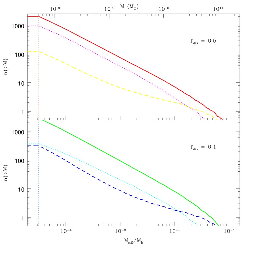
Figure 15: Cumulative initial mass functions for all the subhaloes that merge with a main system between $z=0$ and $z=30$, averaged over many merger trees, for model A ($f_{\rm dis}=0.5$, upper panel) and model B ($f_{\rm dis}=0.1$, lower panel). The solid line shows the mass function of surviving haloes, while the dotted and dashed lines show the mass functions of the subhaloes that have been disrupted by repeated mass loss, and those that have been disrupted by falling into the centre of the potential, respectively. In each case we plot the cumulative number of subhaloes with more than some initial mass which wind up in that final end state.

4.4 Summary

Having examined the dynamical evolution of substructure in a realistic halo, we can conclude on some general features of subhalo dynamics. First, the main dynamical properties of subhaloes are strongly correlated with the quantity $\Delta\,t/P_{\rm rad}$ (where $P_{\rm rad}$ is evaluated at the time when the subhalo first crosses the virial radius of the main system), which provides an estimate of how many radial oscillations they have undergone in the larger system. Younger subhaloes (those with lower values of $\Delta\,t/P_{\rm rad}$) are on less bound and more extended orbits within their parent haloes. The average amount of mass loss, and by implication the degree of tidal stripping, is also strongly correlated with $\Delta\,t/P_{\rm rad}$, as is the fraction of systems that have been disrupted. Disruption also occurs faster on radial orbits, or for more massive satellites. In the next section we will put this information together to suggest a way of treating higher-order substructure in merger trees.

5 A general method for pruning merger trees

When a group of galaxies merges with a larger cluster, the individual galaxies should remain on correlated orbits for some time. Over time, tidal forces and encounters within the cluster will strip the most loosely bound members from the group, so that fewer and fewer objects remain closely associated. After many orbits in the cluster, only tightly bound galaxy pairs will remain associated. Similarly, when a small halo merges into a larger one, its substructure may remain associated, if it is tightly bound, or may be stripped off, if it is loosely bound. Since we expect older substructure to be more tightly bound, and possibly even disrupted, within the infalling halo, we can assume that the substructure stripped off it when it merges into a larger system is preferentially ‘younger’ (in the sense that it has merged into the halo more recently). In what follows, we will outline a pruning method based on this idea.

5.1 Self-similar pruning

5.1.1 How much to prune?

Let us consider the fate of higher-order substructure in a merger tree, say subhaloes within a parent halo that merges with an even larger system. As the parent falls into the large system, it will lose some fraction of its mass, say $\Delta M$, and will be stripped from the outside in. This stripped mass should include subhaloes, since they too can be accelerated away from the parent’s orbit by the tidal field of the larger system. The kinematic distribution of subhaloes within the parent may be biased with respect to its smoothly distributed mass (for instance if subhaloes closer to the centre of the parent have been preferentially disrupted), but we can estimate what fraction $f_{\rm st}$ of the subhaloes are stripped off by determining how they are distributed in radius within the parent, and thus what fraction of the subhaloes are situated in the outer region containing $\Delta M$ of the total mass. If we perform this calculation for $\Delta M=\overline{\Delta M}$, the average mass fraction lost by all subhaloes in the main system up to the present day, then we will have an estimate of the average fraction of substructure stripped off all systems.

The left-hand panel of Fig. 16 shows the average fraction of subhaloes within a given radius, as a function of the fraction of the mass inside that radius, for a large set of model haloes. The two curves are for model A ($f_{\rm dis}=0.5$, solid line) and model B ($f_{\rm dis}=0.1$, dashed line). The satellites are concentrated closer to the centre of the main system in the latter case, but the offset between the two distributions is small. For model A, the average mass fraction lost by subhaloes in the main system is $\overline{\Delta M}=0.33$. The dashed lines indicate that 72 per cent of the subhaloes in a typical halo will lie outside the corresponding radius, that is 72 per cent of all subhaloes lie in the region containing the outermost 33 per cent of the mass. Thus in model A, $f_{\rm st}=0.72$ on average.

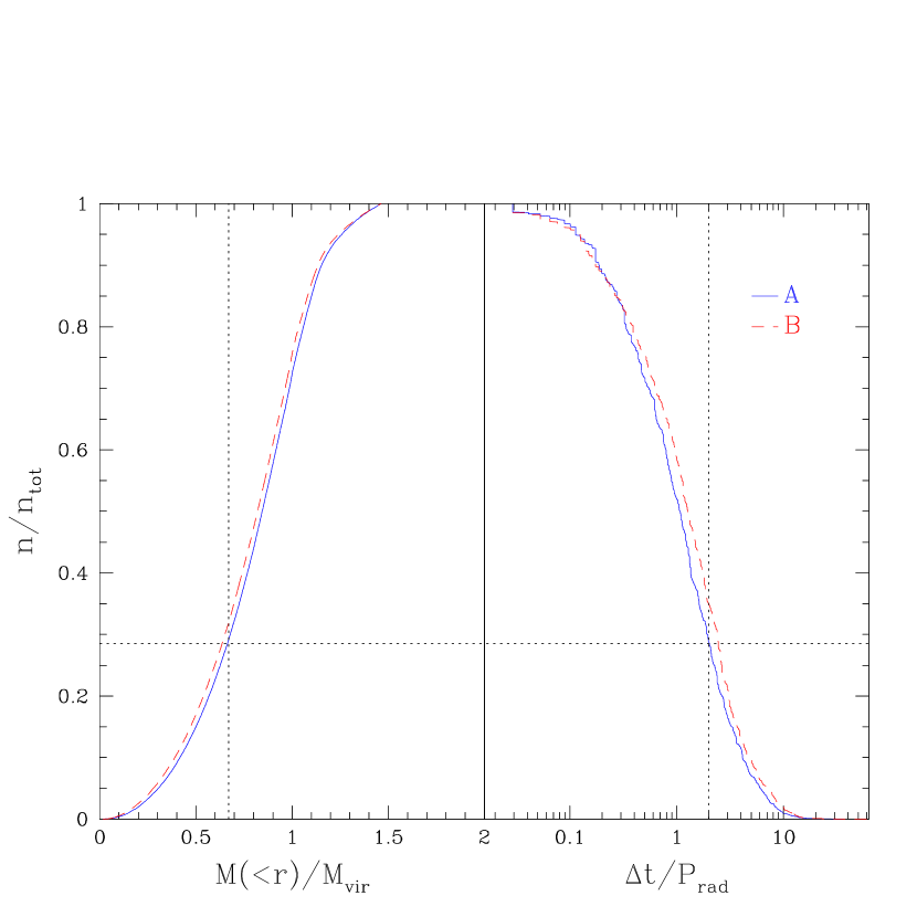
Figure 16: (Left-hand panel) Fraction of systems interior to a given radius, plotted versus the fraction of the total mass of the main system contained within that radius. The two curves are for model A ($f_{\rm dis}=0.5$, solid line) and model B ($f_{\rm dis}=0.1$, dashed line). (Right-hand panel) Fraction of systems which have spent more than a given number of orbits in the system, as a function of $n=\Delta\,t/P_{\rm rad}$. The lines indicate how various fractions of the subhalo population correspond to one another in model A (see text).

5.1.2 Which systems to prune?

In section 4, we saw that younger systems are typically on larger, less bound orbits. If we assume that the subhaloes most recently accreted by the parent will be the first to be stripped off, then we can choose a value $n_{\rm o}$ such that the fraction of subhaloes that have spent less than $n_{\rm o}$ orbits in the parent is equal to $f_{\rm st}$. The right-hand panel of Fig. 16 shows the relative number of subhaloes in a merger tree with $\Delta\,t/P_{\rm rad}>n_{\rm o}$, as a function of $n_{\rm o}$. We see that for $f_{\rm st}=0.72$, $n_{\rm o}=2.0$, that is 72 per cent of the subhaloes in an average halo have spent less than 2 radial periods in their parent system. These are roughly the systems that will be stripped off if the parent loses 33 per cent of its mass. By assuming the most recently acquired haloes are stripped off, we can specify our pruning algorithm in terms of a single parameter, say $n_{\rm o}$. For a given value of $n_{\rm o}$, the corresponding values of $\overline{\Delta M}$ and $f_{\rm st}$ can be determined from the distributions in Fig. 16, or alternately $n_{\rm o}$ and $f_{\rm st}$ can be determined from $\overline{\Delta M}$.

We also saw that orbital properties and disruption rates of satellites depend on the initial circularity of their orbit. We could include this dependence explicitly in our stripping algorithm, but since successive mergers at each level of the hierarchy destroy all information about a satellite’s orbit in earlier systems, we do not lose any precision by averaging over results for different circularities. We should correct for the orbital decay produced by dynamical friction, however; as shown in Fig. 12, the time-scale for this process will be comparable to, or shorter than, 2 radial periods for satellites with masses of $\sim 10^{-2}M_{\rm vir}$ or more, and a substantial fraction of the most massive satellites will be disrupted completely due to orbital decay (cf. Fig. 15). Thus, we revise our pruning criterion slightly, stripping from their parent only those systems that have spent less than $n_{\rm o}$ radial periods in the parent halo, and have orbital decay times longer than $n_{\rm o}\,P_{\rm rad}$. (Based on our mass-loss estimates, and Figs. 9 and 12, we calculate the orbital decay time using equation (13) with a value of $e=2$.)

5.1.3 Fixing parameters

Once we have generated merger trees using initial estimates of $\overline{\Delta M}$, $f_{\rm st}$ and $n_{\rm o}$, we can evolve them and measure new values for these parameters in the main trunk, where we can follow subhalo evolution in detail. If we assume that the evolution of substructure is self-similar in the main trunk and the branches, then iterating through this process will fix the values of the parameters by self-consistency. For a reasonable choice of initial guesses the iteration converges quickly, and we find that for model A, $\overline{\Delta M}=0.32\pm 0.002$ (where the uncertainty is the uncertainty in the average, not the variance of the distribution), $f_{\rm st}=0.71\pm 0.003$ and $n_{\rm o}=2.0\pm 0.05$, while for model B, $\overline{\Delta M}=0.335\pm 0.002$, $f_{\rm st}=0.677\pm 0.003$ and $n_{\rm o}=2.25\pm 0.05$ These averages are determined for all systems over our resolution limit, irrespective of mass. In theory the actual values will depend on our treatment of orbital decay due to dynamical friction, but in practice the averages are completely dominated by low-mass systems, for which dynamical friction is negligible.

Thus we have established a non-parametric method for pruning the side-branches of merger trees. The method is approximative in several ways – for instance we assume subhaloes are stripped off in a strictly first-in-first-out order. We also assume that the properties of substructure, specifically, the average fraction of mass lost by subhaloes, the distribution of their dynamical ages, and their spatial distribution, are self-similar in the main trunk and in the branches of the merger tree. Simulations show that this is roughly true over a wide range of scales, from galaxy haloes to the haloes of massive clusters, so it seems a reasonable approximation. Overall, the method proposed here provides a simple and effective way of handling higher-order substructure in merger trees. In the next section, we will discuss how to implement the method in practice.

5.2 Implementing the method

We can implement the pruning method outlined above as follows. In each side-branch where there is higher-order substructure, we determine for each subhalo the number of orbits it has spent in its initial parent system, measured by $\Delta t/P_{\rm rad}$ (where $P_{\rm rad}$ is evaluated at the time of the subhalo’s original merger with its parent, as in section 4). We also calculate the orbital decay time, from equation (13). If $\Delta t/P_{\rm rad}$ is larger than some number of orbits $n_{\rm o}$, or if the orbital decay time is shorter than $\Delta t$, then we consider the system disrupted within its parent, or so tightly bound that it will not be stripped off its parent subsequently. If $\Delta t/P_{\rm rad}$ is less than $n_{\rm o}$ and the orbital decay time exceeds $\Delta t$, then we assume the system will be stripped from its parent when it merges with a larger halo. We treat the system as a distinct subhalo which merges into the main tree at the same time its parent does, on an associated orbit. Fig. 17 illustrates this pruning process schematically. To fix $n_{\rm o}$, we determine the average amount of mass lost by subhaloes in the main system $\overline{\Delta M}$, and derive the corresponding fraction of subhaloes stripped off along with this mass, $f_{\rm st}$, and number of orbits $n_{\rm o}$ corresponding to $f_{\rm st}$, as explained in the previous section.

Figure 17: A schematic illustration of the pruning process. If a satellite ‘B’ spends less than $n_{\rm o}$ radial periods in the halo of its parent ‘A’ (and if its orbit does not decay), then it is considered to be distinct object associated with ‘A’ when ‘A’ merges with a larger system ‘C’ (bottom figures). Otherwise A and B are treated as a single system (top figures).

There are one or two other details to sort out in this model. First, we must determine what structural parameters to use for higher-order substructure. The concentration of a higher-order subhalo should reflect its original mass and relative age when it first fell into it a parent halo, since it would have stopped growing at this point. These quantities can be determined from the merger tree. While in its parent system (before the merger with the main system), it would also have evolved as described in section 4, losing a fraction $\Delta M_{\rm st}$ of its mass. We can take $\Delta M_{\rm st}$ to be the average fraction of mass lost by subhaloes that have spent less than $n_{\rm o}$ orbits in the main halo (note that this will be less than the average mass-loss fraction for all subhaloes, $\overline{\Delta M}$). Individual subhaloes may be passed on through many levels of the hierarchy, losing mass repeatedly this way until they are disrupted.

With these adjustments made, we now have a full model of halo evolution which, beyond the free parameters $\Lambda_{\rm s}$ and $\epsilon_{\rm h}$ used to describe the evolution of single satellites and fixed by comparison with high-resolution simulations in TB01, has no other major free parameters. The only remaining parametric freedom is in the choice of the disruption criterion $f_{\rm dis}$, and we will show in paper II that this only has a minor effect on the subhalo mass function for reasonable choices of $f_{\rm dis}$. The pruning process can be iterated for successively higher-order branches, producing high-order haloes that may have survived many merging episodes. Fig. 18 shows the average cumulative mass functions of subhaloes of various different orders that merge into a single halo of mass $M_{\rm vir,0}=1.6\times 10^{12}{\rm M}_{\odot}$, (that is the cumulative distribution of their initial masses, when they first merge with the main system). The effect of multiple stripping is clear in the decreasing masses for successively higher-order haloes. We also see that higher-order substructure helps to generate a scale-invariant cumulative mass function at low masses (top-most curve). Even at a mass of $M_{\rm s}=10^{-3}M_{\rm h}$, higher-order substructure accounts for half the subhaloes in a typical system. In paper II we will show that this contribution is required to match the halo mass functions measured in numerical simulations.

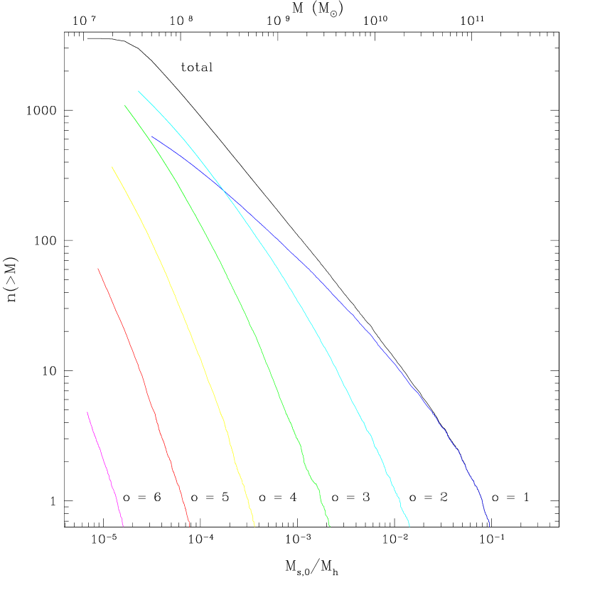
Figure 18: The average cumulative mass function of all subhaloes merging into a system with a present-day mass of $M_{\rm h}=1.6\times 10^{12}{\rm M}_{\odot}$ between $z=0$ and $z=30$ (top line), as well as the contributions from haloes of successively higher order (lower lines, with order increasing from top to bottom).

Pruning with $n_{\rm o}\simeq 2$ also produces the right slope for this power-law tail to the subhalo mass function. Fig. 19 shows input mass functions for basic merger trees where the side-branches are treated as single, monolithic objects (dotted curve), trees pruned with $n_{\rm o}=2.0$ (solid curve), and trees where $n_{\rm o}$ is very large, so that all substructure is counted separately down to the resolution limit of the trees (dashed curve). Pruning transfers some of the material in low-order subhaloes to smaller, higher-order subhaloes, reducing the masses of the former by a small amount while greatly increasing the number of the latter. The net effect on the input mass function is to lower its amplitude slightly at the high-mass end, while steepening the slope considerably at the low-mass end (compare the solid and dotted curves in Fig. 19). In the limit of large $n_{\rm o}$, most of the mass in large systems is decomposed into small systems close to the mass resolution of the merger tree (dashed curve). Subsequent mass loss and disruption will modify these input mass functions, particularly at the high-mass end, as discussed in paper II. Even without considering this subsequent evolution, however, the low-mass slope of the intermediate curve is fairly close to the value of 1.8–2.0 measured in simulations (Ghigna et al. 1998, 2000; Moore et al. 1999; Springel et al. 2001). Finally, higher-order substructure should also introduce orbital correlations in halo substructure. We will consider this point in the next section.

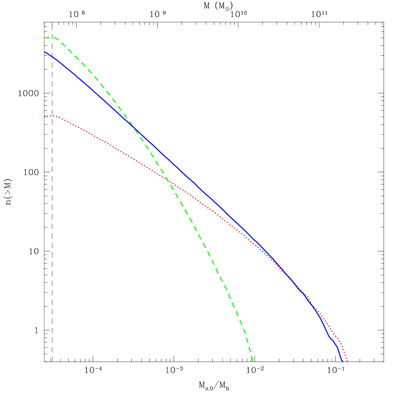
Figure 19: The initial mass function of merging haloes, as in Fig. 18, assuming no pruning, pruning with $n_{\rm o}=2$, and pruning with very large $n_{\rm o}$ (dotted, solid and dashed curves respectively).

5.3 Dynamical groups

When a subhalo that has survived the pruning process merges into the main system alongside its parent, it should have displacements in position and velocity that reflect the size $r_{\rm vir,g}$, mass $M_{\rm g}$, and circular velocity $V_{\rm c,g}$ of the group it falls in with. It is not completely clear how large to make these offsets, since on the one hand we are stripping systems preferentially from the outer parts of the group and the less bound orbits, but on the other hand we cannot account for the self-gravity of the group in our model. In any case, the details of the initial distribution will no longer be relevant after the group has passed through pericentre once and the orbits have been scattered. For simplicity, we will choose an offset in radius picked from a uniform distribution truncated at $\Delta r=r_{\rm vir,g}$ (equivalent to an isothermal density distribution within this radius), and an offset in velocity picked from a Maxwellian distribution of width $\Delta V=V_{\rm c,g}$, with a cutoff at $2\,V_{\rm c,g}$.

These offsets correspond to the approximate spatial and velocity distributions of substructure in hierarchically assembled haloes, so in effect we are simply putting realistic haloes with multiple components into the main potential. A slightly different interpretation of the offsets is that groups lose material, just as as individual haloes do, into streams with a characteristic initial scale comparable to $r_{\rm vir,g}$ and a velocity dispersion comparable to $V_{\rm c,g}$ (see for instance Johnston 1998). Of course, the short-coming of this method is that the subsequent evolution of the group neglects its self-gravity, as mentioned previously, and thus the total velocity dispersion of our haloes may be slightly larger than it should be. We will discuss this further in paper II.

Having included this description of orbital correlations in our model, we now have a way of studying groups of substructure within larger systems. Fig. 20, for instance, shows a few young groups in a halo that has experienced many recent mergers. Similar substructure can be observed both in galaxy clusters, particularly with the recent availability of high-resolution X-ray imaging and multi-object spectroscopy (e.g. Sun, Murray, Markevitch, & Vikhlinin 2002; Mazzotta, Fusco-Femiano, & Vikhlinin 2002; Berrington, Lugger, & Cohn 2002; Belsole et al. 2002; Bardelli et al. 2002) and even in the halo of Milky Way, where the Magellanic Clouds and some of the other satellites appear to be members of dynamical groups on associated orbits (Lynden-Bell 1976; see Binney 2001, and Palma, Majewski, & Johnston 2002 for recent references). There is the intriguing possibility of reconstructing the merger history of our galaxy using these observed groups, particularly if more accurate kinematic information becomes available through interferometric satellites such as GAIA (Binney 2001). We will consider the properties and evolution of dynamical groups further in paper II.

Figure 20: The projected positions of the members of several young groups, in a halo that has experienced many recent mergers. The large symbols are group members, with point type indicating group membership and point size giving an indication of mass; the small dots are the other subhaloes in the system.

6 Summary

There is increasing evidence, both observational and theoretical, that the dark matter haloes surrounding galaxies, groups and clusters contain substructure on a wide range of scales. It is beyond current computational capabilities to determine the properties of this substructure directly. To take full advantage of results from lensing observations, dark matter direct-detection experiments, and searches for a WIMP annihilation signal in the gamma-ray background, and to provide a robust platform for detailed models of small-scale structure formation in general cosmologies, an analytic or semi-analytic extension to current numerical methods is required. A key problem in devising such a model is to determine how much substructure to pass on from one level of the merger hierarchy to the next.

In this paper, we have applied the analytic model of satellite evolution developed in TB01 to the study of merging haloes, using the initial conditions for these mergers expected in a cosmological setting. We find that several basic patterns characterise subhalo dynamics. The main time-scale for subhalo evolution is the period for radial oscillations at the virial radius, $P_{\rm rad}\simeq 5\,r_{\rm vir}/V_{\rm c}$ (evaluated at the time when the subhalo first crosses the virial radius of the main system), since this is the period for successive pericentric passages in the satellite’s orbit. Around each pericentric passage, the subhalo loses mass through tidal stripping; for representative densities and density profiles roughly 25–45 per cent of the remaining mass is lost on each successive orbit, the exact fraction depending on the circularity of the orbit and the concentration of the satellite. After 5–10 orbits, systems may be disrupted completely by this repeated mass loss. Orbital decay due to dynamical friction is also an important factor in subhalo evolution, but only for the most massive subhaloes, those with a few per cent of the mass of the main system or more.

Considering the average properties of subhaloes in realistic systems, generated using semi-analytic merger trees, we find correlations between the merger epoch of the subhalo, its average orbital radius, and to a lesser extent its orbital energy. Based on this correlation, and on the observation that haloes are stripped of their mass from the inside out (e.g. Hayashi et al. 2003), we suggest a method for ‘pruning’ merger trees, that is determining how much distinct substructure should be passed on from one level of the merging hierarchy to the next.

When haloes with substructure merge into larger systems, they should lose mass just as simple haloes do. This mass will include some self-bound substructure, so tidal stripping should produce groups of independent subhaloes on orbits similar to that of the original parent. To determine how much substructure to strip from a parent, we assume self-similarity in the merger tree. On average, a parent in a side-branch should lose a fraction of its mass that can be determined directly from the evolution of satellites in the main halo in our model. Assuming that this mass is stripped from the outside in, and that the outer material consists of the most recently accreted substructure, we determine that subhaloes should be passed down the merger tree if they have spent less than $n_{\rm o}\simeq 2$ orbits in their parent halo by the time it merges with a larger system, and that they should be subsumed into their parent otherwise. The critical number of orbits $n_{\rm o}$ is initially a free parameter in our model, but we can fix it iteratively by requiring that our model be self-consistent, that is by assuming the same average properties for subhaloes in the side-branches as are measured directly for subhaloes in the main trunk of the merger tree.

Obviously, the ultimate value of our method rests on how well it reproduces the results of high-resolution simulations of halo substructure, for standard cosmologies. In paper II, we will test our method by comparing to a series of simulations of galaxy and cluster haloes. We will show that in general there is reasonable agreement between the two methods, but that we see a few discrepancies between the numerical and the semi-analytic results. We will argue that some of these discrepancies may actually be due to numerical effects in the simulations, and that overall, our method provides a reliable estimate of small-scale substructure within dark matter haloes.

References

- [Aloisio, Blasi, Olinto(2002)] Aloisio R., Blasi P., Olinto A. V., 2002, preprint (astro-ph/0206036)
- [Arabadjis, Bautz, Garmire(2002)] Arabadjis J. S., Bautz M. W., Garmire G. P., 2002, ApJ, 572, 66
- [Bardelli et al.(2002)] Bardelli S., Venturi T., Zucca E., De Grandi S., Ettori S., Molendi S., 2002, AAp, 396, 65
- [Benson et al.(2002a)] Benson A. J., Lacey C. G., Baugh C. M., Cole S., Frenk C. S., 2002, MNRAS, 333, 156
- [Benson et al.(2002b)] Benson A. J., Frenk C. S., Lacey C. G., Baugh C. M., Cole S., 2002, MNRAS, 333, 177
- [Belsole, Ferrari, Bourdin, Pratt(2002)] Belsole E., Ferrari C., Bourdin H., Pratt G., 2002, in Combes F., Barret D., eds, SF2A-2002: Semaine de l’Astrophysique Francaise. EdP-Sciences (Editions de Physique), Les Ulis, France
- [1] Bergström L., 2000, Rept. Prog. Phys. 63, 793
- [Bergström, Edsjö, Ullio (2001)] Bergström L., Edsjö J., Ullio P., 2001, Phys. Rev. Lett. 87, 251301
- [Berrington, Lugger, Cohn(2002)] Berrington R. C., Lugger P. M., Cohn H. N., 2002, AJ, 123, 2261
- [Binney(2001)] Binney J., 2001, in Deiters S., Fuchs B., Spurzem R., Just A., Wielen R., eds, ASP Conf. Ser. 228: Dynamics of Star Clusters and the Milky Way. Astron. Soc. Pac., San Fransico, p. 269
- [Binney, Tremaine(1987)] Binney J., Tremaine S., 1987, Galactic Dynamics. Princeton University Press, Princeton, NJ
- [Blais-Ouellette, Amram, Carignan(2001)] Blais-Ouellette S., Amram P., Carignan C., 2001, AJ, 121, 1952
- [Blasi, Sheth(2001)] Blasi P., Sheth R. K., 2001, Technical Report, DE2001-787842, 2, 16370
- [Blumenthal, Faber, Primack, Rees(1984)] Blumenthal G. R., Faber S. M., Primack J. R., Rees M. J., 1984, Nature, 311, 517
- [Bœhm, Riazuelo, Hansen, Schaeffer(2002)] Bœhm C., Riazuelo A., Hansen S. H., Schaeffer R., 2002, Phys. Rev. D, 66, 83505
- [Bond et al.1991] Bond J.R., Cole S., Efstathiou G., Kaiser N., 1991, ApJ, 379, 440
- [Borriello, Salucci] Borriello A., Salucci P., 2001, MNRAS, 323, 285
- [Bower 1991] Bower R.G., 1991, MNRAS, 248, 332
- [Bradač et al.(2002)] Bradač M., Schneider P., Steinmetz M., Lombardi M., King L. J., Porcas R., 2002, AAp, 388, 373
- [Bullock, Kravtsov, Weinberg(2000)] Bullock J. S., Kravtsov A. V., Weinberg D. H., 2000, ApJ, 539, 517
- [Bullock, Kravtsov, Weinberg(2001a)] Bullock J. S., Kravtsov A. V., Weinberg D. H., 2001, ApJ, 548, 33
- [Bullock et al.(2001b)] Bullock J. S., Kolatt T. S., Sigad Y., Somerville R. S., Kravtsov A. V., Klypin A. A., Primack J. R., Dekel A., 2001, MNRAS, 321, 559
- [Cálcáneo-Roldan, Moore(2000)] Cálcáneo-Roldan C., Moore B., 2000, Phys. Rev. D62, 123005
- [Chandrasekhar(1943)] Chandrasekhar S., 1943, ApJ, 97, 255
- [Chiba(2002)] Chiba M., 2002, ApJ, 565, 17
- [Cole 1991] Cole S., 1991, ApJ, 367, 45
- [Cole et al.1994] Cole S., Aragon-Salamanca A., Frenk C.S., Navarro J.F., Zepf S.E., 1994, MNRAS, 271, 781
- [Cole, Lacey, Baugh, Frenk(2000)] Cole S., Lacey C. G., Baugh C. M., Frenk C. S., 2000, MNRAS, 319, 168
- [Colpi, Mayer, Governato(1999)] Colpi M., Mayer L., Governato F., 1999, ApJ, 525, 720
- [Cyburt, Fields, Pavlidou, Wandelt(2002)] Cyburt R. H., Fields B. D., Pavlidou V., Wandelt B., 2002, Phys. Rev. D, 65, 123503
- [David et al.(2001)] David L. P., Nulsen P. E. J., McNamara B. R., Forman W., Jones C., Ponman T., Robertson B., Wise M., 2001, ApJ, 557, 546
- [Dalal, Kochanek(2002)] Dalal N. , Kochanek C. S., 2002, ApJ, 572, 25
- [de Blok, Bosma(2002)] de Blok W. J. G., Bosma A., 2002, AAp, 385, 816
- [Eke, Cole, Frenk 1996] Eke V.R., Cole S.M., Frenk C.S., 1996, MNRAS, 282, 263
- [Eke, Navarro, Steinmetz(2001)] Eke V. R., Navarro J. F., Steinmetz M., 2001, ApJ, 554, 114
- [Font, Navarro, Stadel, Quinn(2001)] Font A. S., Navarro J. F., Stadel J., Quinn T., 2001, ApJ, 563, L1
- [Fukushige, Makino(2001)] Fukushige T. , Makino J., 2001, ApJ, 557, 533
- [Ghigna et al.(1998)] Ghigna S., Moore B., Governato F., Lake G., Quinn T., Stadel J., 1998, MNRAS, 300, 146
- [Ghigna et al.(2000)] Ghigna S., Moore B., Governato F., Lake G., Quinn T., Stadel J., 2000, ApJ, 544, 616
- [Gnedin, Ostriker(1999)] Gnedin O. Y., Ostriker J. P., 1999, ApJ, 513, 626
- [Gondolo, Silk(1999)] Gondolo P., Silk J., 1999, Phys. Rev. Let., 83, 1719
- [Governato, Ghigna, Moore(2001)] Governato F., Ghigna S., Moore B., 2001, in ASP Conf. Ser. 245: Astrophysical Ages and Times Scales, 469
- [Goodman(2000)] Goodman J., 2000, New Astronomy, 5, 103
- [Hatton et al.(2003)] Hatton S., Devriendt J. E. G., Ninin S., Bouchet F. R., Guiderdoni B., Vibert D., 2003, in preparation (http://galics.iap.fr)
- [2] Hayashi E., Navarro J. F., Taylor J. E., Stadel J., Quinn T., 2003, ApJ, in press (astro-ph/0203004)
- [Helmi, White, Springel(2002)] Helmi A., White S. D., Springel V., 2002, Phys. Rev. D, 66, 63502
- [Hoekstra, Franx, Kuijken, van Dokkum(2002)] Hoekstra H., Franx M., Kuijken K., van Dokkum P. G., 2002, MNRAS, 333, 911
- [Hu, Barkana, Gruzinov(2000)] Hu W., Barkana R., Gruzinov A., 2000, Phys. Rev. Let., 85, 1158
- [Ibata, Lewis, Irwin, Quinn(2002)] Ibata R. A., Lewis G. F., Irwin M. J., Quinn T., 2002, MNRAS, 332, 915
- [Jenkins et al.(2001)] Jenkins A., Frenk C. S., White S. D. M., Colberg J. M., Cole S., Evrard A. E., Couchman, H. M. P., Yoshida N., 2001, MNRAS, 321, 372
- [Johnston(1998)] Johnston K. V., 1998, ApJ, 495, 297
- [Johnston, Spergel, Haydn(2002)] Johnston K. V., Spergel D. N., Haydn C., 2002, ApJ, 570, 656
- [Kauffmann, White(1993)] Kauffmann G., White S. D. M., 1993, MNRAS, 261, 921
- [] Kauffmann G., White S.D.M., Guiderdoni B., 1993, MNRAS, 264, 201
- [] Keeton C. R., 2002, preprint (astro-ph/0111595)
- [Klypin, Gottlöber, Kravtsov, Khokhlov(1999)] Klypin A., Gottlöber S., Kravtsov A. V., Khokhlov A. M., 1999, ApJ, 516, 530
- [Klypin, Zhao, Somerville(2002)] Klypin A., Zhao H., Somerville R. S., 2002, ApJ, 573, 597
- [Kochaneck 1995] Kochaneck C.S., 1995, ApJ, 453, 545
- [Lacey, Cole 1993] Lacey C., Cole S., 1993, MNRAS, 262, 627
- [Lacey, Cole 1994] Lacey C., Cole S., 1994, MNRAS, 271, 676
- [Lewis, Buote, Stocke] Lewis A. D., Buote D. A., Stocke J. T., 2002, ApJ, submitted (astro-ph/0209205)
- [Lynden-Bell 1976] Lynden-Bell D., 1976, MNRAS, 174, 695
- [Maoz 1990] Maoz E., 1990, ApJ, 359, 257
- [Marchesini et al.(2002)] Marchesini D., D’Onghia E., Chincarini G., Firmani C., Conconi P., Molinari E., Zacchei A., 2002, ApJ, 575, 801
- [Mayer et al.(2002)] Mayer L., Moore B., Quinn T., Governato F., Stadel J., 2002, MNRAS, 336, 119
- [Mazzotta, Fusco-Femiano, Vikhlinin(2002)] Mazzotta P., Fusco-Femiano R., Vikhlinin A., 2002, ApJ, 569, L31
- [Menci et al.(2002)] Menci N., Cavaliere A., Fontana A., Giallongo E., Poli F., 2002, ApJ, 575, 18
- [Metcalf(2002)] Metcalf R. B., 2002, ApJ, 580, 696
- [Metcalf, Madau(2001)] Metcalf R. B., Madau P., 2001, ApJ, 563, 9
- [Metcalf, Zhao(2002)] Metcalf R. B., Zhao H., 2002, ApJ, 567, L5
- [Moore et al.(1998)] Moore B., Governato F., Quinn T., Stadel J., Lake G., 1998, ApJ, 499, L5
- [Moore et al.(1999)] Moore B., Ghigna S., Governato F., Lake G., Quinn T., Stadel J., Tozzi P., 1999, ApJ, 524, L19
- [Natarajan, Loeb, Kneib, Smail(2002)] Natarajan P., Loeb A., Kneib J., Smail I., 2002, ApJ, 580, L17
- [Navarro, Frenk, White(1995)] Navarro J. F., Frenk C. S., White S. D. M., 1995, MNRAS, 275, 56
- [3] Navarro J.F., Frenk C.S., White S.D.M., 1996, ApJ, 462, 563
- [4] Navarro J.F., Frenk C.S., White S.D.M., 1997, ApJ, 490, 493
- [Okamoto, Habe(1999)] Okamoto T., Habe A., 1999, ApJ, 516, 591
- [Padmanabhan(1993)] Padmanabhan T., 1993, Structure Formation in the Universe. Cambridge University Press, Cambridge, UK
- [Padmanabhan, Choudhury(2002)] Padmanabhan T., Choudhury T. R., 2002, Phys. Rev. D, 66, 81301
- [Palma, Majewski, Johnston(2002)] Palma C., Majewski S. R., Johnston K. V., 2002, ApJ, 564, 736
- [Peebles(1969)] Peebles P. J. E., 1969, ApJ, 155, 393
- [Peebles 1980] Peebles P.J.E., 1980, The Large Scale Structure of the Universe. Princeton University Press, Princeton, NJ
- [Peebles, Vilenkin(1999)] Peebles P. J. E., Vilenkin A., 1999, Phys. Rev. D, 60, 103506
- [Power et al.(2003)] Power C., Navarro J. F., Jenkins A., Frenk C. S., White S. D. M., Springel V., Stadel, J., Quinn T., 2003, MNRAS, 338, 14
- [Press, Schechter(1974)] Press W. H., Schechter P., 1974, ApJ, 187, 425
- [Pretzl(2002)] Pretzl K., 2002, Space Science Reviews, 100, 209
- [Sand, Treu, Ellis(2002)] Sand D. J., Treu T., Ellis R. S., 2002, ApJ, 574, L129
- [Sheth, Lemson(1999)] Sheth R. K., Lemson G., 1999, MNRAS, 305, 946
- [Sheth, Tormen(1999)] Sheth R. K., Tormen G., 1999, MNRAS, 308, 119
- [Somerville(2002)] Somerville R. S., 2002, ApJ, 572, L23
- [Somerville, Kolatt(1999)] Somerville R. S., Kolatt T. S., 1999, MNRAS, 305, 1
- [Somerville, Primack(1999)] Somerville R. S., Primack J. R., 1999, MNRAS, 310, 1087
- [Somerville, Lemson, Kolatt, Dekel(2000)] Somerville R. S., Lemson G., Kolatt T. S., Dekel A., 2000, MNRAS, 316, 479
- [Spergel, Steinhardt(2000)] Spergel D. N., Steinhardt P. J., 2000, Phys. Rev. Let., 84, 3760
- [Springel, White, Tormen, Kauffmann(2001)] Springel V., White S. D. M., Tormen G., Kauffmann G., 2001, MNRAS, 328, 726
- [Stoehr, White, Tormen, Springel(2002)] Stoehr F., White S. D. M., Tormen G., Springel V., 2002, MNRAS, 335, L84
- [Sun, Murray, Markevitch, Vikhlinin(2002)] Sun M., Murray S. S., Markevitch M., Vikhlinin A., 2002, ApJ, 565, 867
- [Taffoni, Mayer, Colpi, Governato(2002)] Taffoni G., Mayer L., Colpi M., Governato F., 2002, in Fusco-Femiano R., Matteucci F., eds, ASP Conf. Ser. 253: Chemical Enrichment of Intracluster and Intergalactic Medium. Astron. Soc. Pac., San Fransico, p. 273
- [Taylor (2001)] Taylor J. E., 2001, PhD thesis, University of Victoria
- [Taylor, Babul(2001)] Taylor J. E., Babul A., 2001, ApJ, 559, 716
- [Taylor, Navarro(2001)] Taylor J. E., Navarro J. F., 2001, ApJ, 563, 483
- [Taylor, Silk (2002)] Taylor J. E., Silk J., 2002, MNRAS, in press (astro-ph/0207299)
- [Tormen 1997] Tormen G., 1997, MNRAS, 300, 773
- [Toth, Ostriker(1992)] Tóth G., Ostriker J. P., 1992, ApJ, 389, 5
- [Ullio, Bergström, Edsjö, Lacey(2002)] Ullio P., Bergström L., Edsjö J., Lacey C., 2002, preprint (astro-ph/0207125)
- [van den Bosch, Lewis, Lake, Stadel(1999)] van den Bosch F. C., Lewis G. F., Lake G., Stadel J., 1999, ApJ, 515, 50
- [Velazquez, White(1999)] Velázquez H., White S. D. M., 1999, MNRAS, 304, 254
- [Vitvitska et al.(2002)] Vitvitska M., Klypin A. A., Kravtsov A. V., Wechsler R. H., Primack J. R., Bullock J. S., 2002, ApJ, 581, 799
- [Wechsler et al.(2002)] Wechsler R. H., Bullock J. S., Primack J. R., Kravtsov A. V., Dekel A., 2002, ApJ, 568, 52
- [Wetterich(2002)] Wetterich C., 2002, Phys. Rev. D, 65, 123512
- [White, Rees(1978)] White S. D. M., Rees, M. J., 1978, MNRAS, 183, 341
- [Zhao et al. (2002)] Zhao D., Mo H., Jing Y., Boerner G., 2002, MNRAS, in press (astro-ph/0204108)