Multiple UHECR Events from Galactic hadron jets

Abstract

We propose a new observational test of top-down source models for the ultra-high-energy cosmic-rays (UHECRs), based on the simultaneous observation of two or more photons from the same Galactic hadron jet. We derive a general formula allowing one to calculate the probability of detecting such ‘multiple events’, for any particular top-down model, once the physical parameters of the associated hadron jets are known. We then apply our results to a generic top-down model involving the decay of a supermassive particle, and show that under reasonable assumptions the next-generation UHECR detectors would be able to detect multiple events on a timescale of a few years, depending on the mass of the top-down progenitor. Either the observation or the non-observation of such events will provide constraints on the UHECR top-down models and/or the physics of hadronization at ultra-high energy.

1 Introduction

Ultra-high-energy cosmic rays (UHECRs) are puzzling in respect of both their production and their propagation in the universe. On the one hand, even the most powerful astrophysical sites known to be able to accelerate particles to very high energy seem to have difficulties to reach energies as high as $3\times 10^{20}$ eV (the highest reported UHECR energy so far[1]). On the other hand, even if they could, one would expect from the (presumably) extremely high rigidity of the observed UHECRs in the intergalactic medium that their directions of arrival in the Earth atmosphere roughly point towards the sources, which does not seem to be the case. Also, it had been expected that the UHECR flux above $\sim 10^{20}$ eV would be very much reduced due to the interaction of the UHE particles with the cosmological microwave background. This so-called GZK cutoff[2], however, does not seem to be present in the currently available data.

Although the UHECR sources are still essentially unknown, many models have been proposed, with various charms and problems [3]. They can be divided up into two classes: bottom-up models, in which particles initially at low (thermal) energy get accelerated by one or a series of astrophysical processes, and top-down models, in which each UHECR is directly produced, as a particle, at ultra-high energy, through the decay of a pre-existing supermassive particle or some exotic, high-energy physical process, e.g. involving the collapse or annihilation of topological defects. In this paper, we consider the so-called Galactic top-down models from a general point of view, merely assuming that the UHECR flux is dominated by sources in the Halo, with a density proportional to that of the dark matter. This solves the ‘production problem’ trivially (or more exactly shifts it to the problem of identifying the X-particles and explaining their production and decay rates) and provides a simple understanding of the absence of a GZK cutoff as well as the apparent isotropy of the UHECRs – at least until the statistics will be high enough for us to detect the dipole anisotropy due to the off-centered position of the solar system in the Galaxy (which should take at least three years of observation with the Pierre Auger Observatory (PAO) [5]).

Many different models have been proposed, with X-particles of different types (either produced locally, notably through topological defect interactions, or inherited from the big bang) and different masses (on the Planck scale, $10^{28}$ eV, the GUT scale, $10^{25}$ eV, or below) [3, 6]. In this paper, we investigate a common consequence of a large class of Galactic top-down models, and propose an observational test which could be accessible to the next generation of UHECR detectors, such as the PAO [7], the EUSO experiment [8] or the OWL/AirWatch project [9].

2 Multiple UHECR events: the basic idea

Top-down scenarios involve the production of hadron jets in a way similar to what is observed in terrestrial accelerators, when an energetic quark-antiquark pair (e.g. produced through e⁺e^- annihilation) hadronizes into a number of colourless hadrons through a QCD cascade. Let $N_{\gamma}$ be the number of photons in a jet (from neutral pion decay), and $\theta_{\mathrm{jet}}$ be the jet opening angle. Since gamma-rays propagate in straight lines away from the source, the average surface density of UHE photons at a distance $D$ from the point where the X-particle decayed is $\sigma=N_{\gamma}/\omega_{\mathrm{jet}}D^{2}$, where $\omega_{\mathrm{jet}}\simeq\pi\theta_{\mathrm{jet}}^{2}$ is the jet solid angle. If a detector intersects such a jet, with a surface area $S_{\perp}$ orthogonal to the jet axis, it will see on average the following number of particles:

$$\mu=\frac{N_{\gamma}S_{\perp}}{\pi\theta_{\mathrm{jet}}^{2}D^{2}}.$$ (1)

If the source is close enough, the number of photons in the jet high enough and the detector surface large enough, then $\mu$ will be larger than one and several UHECRs will be able to cross the detector at (almost exactly) the same time, from (almost exactly) the same direction. This is what we define to be a multiple event. It has an unambiguous experimental signature: two or more distinct showers developing simultaneously in the atmosphere, with almost perfectly parallel axes (within $\sqrt{S_{\perp}}/D$ radians, which is much less than any conceivable experimental angular resolution).

The number $\mu$ may be called the multiplicity of the X-particle decay event, or more exactly its potential multiplicity, as can be expected at Earth, since it is the average number of particles which can be observed simultaneously by the detector (assuming that it intersects the jet). For a given X-particle decay event, with a given $\mu$, the actual multiplicity of the UHECR event as observed by the detector can only be predicted statistically. The probability, $\mathcal{P}(m,\mu)$, of observing an event with actual multiplicity $m$ (integer) in a jet of potential multiplicity $\mu$ (real number) is given by the binomial law:

$$\mathcal{P}(m,\mu)=C_{N_{\gamma}-1}^{m-1}\left(\frac{\mu}{N_{\gamma}}\right)^{m-1}\left(1-\frac{\mu}{N_{\gamma}}\right)^{N_{\gamma}-m},$$ (2)

where $\mu/N_{\gamma}=S_{\perp}/S_{\mathrm{jet}}$ is the ratio of the detector’s surface to the jet surface (see Eq. (1)), and thus the probability for a given particle in the jet to cross the detector. Note that $\mathcal{P}(m,\mu)$ is actually the conditional probability of the multiple event, given the fact that one shower is observed, or if one prefers, the probability that a detected shower be accompanied by $m-1$ others. The probability of observing a multiple event with whatever multiplicity larger than two simply adds up to $\mathcal{P}(m\geq 2,\mu)=1-(1-\mu/N_{\gamma})^{N_{\gamma}-1}\approx 1-e^{-\mu}$, for not too small values of $N_{\gamma}$.

The basic idea behind top-down multiple events is thus that the UHECRs are not independent of one another, but appear in close groups released at the same time in a single X-particle decay event. If the groups are sufficiently tight, we should be able to detect several UHECRs at a time. In fact, top-down jets can be seen as genuine Galactic showers: in the same way as we detect single UHECR events by intercepting many secondary particles belonging to the same atmospheric shower, the use of very large detectors may allow us to detect single ‘X-particle decay events’ by intercepting several UHECRs belonging to the same Galactic shower. The detectability of multiple events thus comes down to the question: when we see one UHECR in a top-down jet, how close is the next one, compared to the detector’s radius?

3 Timescale of multiple event detection

The potential multiplicity, $\mu$, of a UHECR event (Eq. 1) depends on two physical parameters related to the jet properties, $N_{\gamma}$ and $\theta_{\mathrm{jet}}$, one astrophysical parameter, $D$, related to the source distribution, and one ‘experimental’ parameter, $S_{\perp}$, related to the detector. Most X-particle decays will occur much too far from the solar system to give rise to multiple events. But if one assumes that the X-particles distribute over the Galactic halo in the same way as the dark-matter, one can estimate the probability that one of the many UHECR events that will be detected over a given period of observation corresponds to a small enough source distance.

Figure 1: Effective source density for various models of the dark-matter distribution in our Galaxy. Labels indicate the assumed value of $R_{\mathrm{c}}$ for either isothermal or FRW models (see text).

3.1 The distribution of source distances

The statistics of multiple events depend on that of source distances. For the dark-matter distribution in the Galaxy, we may consider either a simple isothermal halo model [11], where the density, $n_{\mathrm{DM}}$ depends on the galactocentric distance, $r$, proportionally to $1/(r^{2}+R_{\mathrm{c}}^{2})$, and the core radius $R_{\mathrm{c}}$ is of the order of a few kiloparsecs, or an FRW model based on cold dark matter simulations, with $n_{\mathrm{DM}}\propto 1/[r(r+R_{\mathrm{c}})^{2}]$ [12]. In Fig. 1, we have plotted the corresponding effective UHECR source density as a function of distance, for an observer located at the galactocentric radius of the Sun (taking into account the smaller effective contribution of more distant sources).

As can be seen, the effective source density is flat for low values of the source distance, which are those of interest to us because they give the highest probability of observing multiple events. This result is nothing but the famous Olber’s paradox, and it is independent of the actual dark matter distribution, provided it is not varying significantly on small scales. Moreover, the actual density profile of the dark matter halo appears not to affect significantly the normalization of the source density at small distances (except for unreasonable values of $R_{\mathrm{c}}$). In the following, we adopt the value of $6\times 10^{-5}\,\mathrm{pc}^{-1}$ (recalling that NRF models are currently preferred) and replace, for all practical purposes of the present study, the effective distribution of UHECR source distances by the following differential probability:

$$\mathrm{d}\mathrm{P}(D)=p(D)\mathrm{d}D=\frac{1}{D_{0}}\mathrm{d}D\quad\quad(0\leq D\leq D_{0}),$$ (3)

where $D_{0}=1/(6\times 10^{-5})\simeq 17$ kpc is an effective radius beyond which no UHECR sources exist (that is, they contribute a negligible flux at Earth).

Note that inhomogeneities in the dark matter distribution may in practice alter the probability of X-particle decay events at a given point of the Galaxy. A lower concentration of sources close to the Earth would decrease the chance of detecting multiple events, while a higher concentration would increase it. Lacking a precise knowledge of the small scale dark matter distribution, we can but assume that the Earth environment is not very different from the average.

3.2 Multiple event probability

For convenience, we shall rewrite the potential multiplicity of an individual UHECR event, given by Eq. (1), as:

$$\mu(D)=\mu_{0}\frac{D_{0}^{2}}{D^{2}},\quad\mathrm{where}\quad\mu_{0}=\frac{N_{\gamma}S_{\perp}}{\pi\theta_{\mathrm{jet}}^{2}D_{0}^{2}}.$$ (4)

For any given model, the probability of detecting an event of actual multiplicity larger than $n$ increases with the total number of UHECR events detected, $N_{\mathrm{evt}}$, according to the simple law:

$$\mathcal{P}_{\geq n}(N_{\mathrm{evt}})=1-e^{-\frac{N_{\mathrm{evt}}}{N_{n}}},$$ (5)

where the constants $N_{n}$ are the characteristic numbers of events which have to be detected before it becomes reasonably probable ($\sim 63\%$) to detect an event of multiplicity $n$. This is a straightforward consequence of the statistical independence of X-particle decay events (see Appendix).

We show in the appendix that the characteristic event number for double event detection is given by :

$$N_{2}=\frac{1}{\sqrt{\pi}}\mu_{0}^{-1/2},$$ (6)

and that the subsequent numbers deduce from $N_{2}$ by the following recursion relation (valid for detected multiplicities much smaller than the total jet multiplicity, $n\ll N_{\gamma}$):

$$N_{n+2}=\frac{2n}{2n-1}N_{n+1},$$ (7)

so that, in particular, $N_{3}=2N_{2}$, $N_{4}=\frac{4}{3}N_{3}$, $N_{5}=\frac{6}{5}N_{3}$, etc.

3.3 Multiple event detection timescales

In order to convert the above characteristic event numbers into multiple event detection timescales (for a given detector), we just need to calculate the UHECR detection rate. This depends on the total aperture, $\mathcal{A}_{\mathrm{d}}$ (in $\mathrm{km}^{2}\mathrm{sr}$), and the duty cycle, $\delta$ (in percent), of the detector. The UHECR detection rate above energy $E$ is given by:

$$\dot{N}_{\mathrm{evt}}(\geq E)=\Phi_{\mathrm{CR}}(\geq E)\times\mathcal{A}_{\mathrm{d}}\times\delta\,,$$ (8)

where $\Phi_{\mathrm{CR}}(\geq E)$ is the integral flux of UHECRs above energy $E$. From the AGASA and Fly’s Eye experiments, a fair value of the UHECR flux at $10^{20}$ eV is $\Phi_{\mathrm{CR}}(10^{20})\simeq 3\times 10^{-40}\,\mathrm{cm}^{-2}\mathrm{s}^{-1}\mathrm{sr}^{-1}\mathrm{eV}^{-1}$. The intergal flux obviously depends on the actual spectrum, which is virtually unknown above $10^{20}$ eV. As for the spectrum below that energy, one should keep in mind that we are only interested in the events which can be attributed to the top-down process under consideration, and which probably represent only a fraction of the total detected events between $10^{19}$ and $10^{20}$ eV. We shall note $\Phi^{\mathrm{td}}_{\geq E_{\mathrm{th}}}$ the corresponding integrated flux above the detector’s threshold energy, $E_{\mathrm{th}}$.

We can now express the time evolution of the multiple event probabilities, by replacing $N_{\mathrm{evt}}$ by $\dot{N}_{\mathrm{evt}}\times t$ in Eq. (5):

$$\mathcal{P}_{\geq n}(t)=1-e^{-\frac{t}{\tau_{n}}},\quad\mathrm{where}\quad\tau_{n}=N_{n}/\dot{N}_{\mathrm{evt}}.$$ (9)

Using Eqs. (6) and (8) and the expression for $\mu_{0}$, Eq. (4), we find:

$$\tau_{2}=\frac{\theta_{\mathrm{jet}}(E_{\mathrm{th}})\,D_{0}}{N_{\gamma,\geq E_{\mathrm{th}}}^{1/2}\left<S_{\perp}\right>^{1/2}\Phi^{\mathrm{td}}_{\geq E_{\mathrm{th}}}\mathcal{A}_{\mathrm{d}}\delta}\,\,,\quad\mathrm{and}\quad\tau_{n+2}=\frac{2n}{2n-1}\tau_{n+1}.$$ (10)

In practice, the average perpendicular surface of the detector, $\left<S_{\perp}\right>$, is related to the acceptance $\mathcal{A}_{\mathrm{d}}$. If the detector’s surface on the ground is $S_{\mathrm{d}}$, and $\theta_{\mathrm{max}}$ is the maximum zenith angle visible by the detector, we have $\left<S_{\perp}\right>=\frac{1}{2}S_{\mathrm{d}}\times\sin^{2}\theta_{\mathrm{max}}/(1-\cos\theta_{\mathrm{max}})$, and $\mathcal{A}_{\mathrm{d}}=S_{\mathrm{d}}\times\pi\sin^{2}\theta_{\mathrm{max}}$. If $\theta_{\mathrm{max}}=90\hbox{${}^{\circ}$}$, $\left<S_{\perp}\right>=\tfrac{1}{2}S_{\mathrm{d}}$, and $\mathcal{A}_{\mathrm{d}}=\pi S_{\mathrm{d}}$. Reporting into Eq. (10), we get:

$$\tau_{2}=\frac{\sqrt{2}\,\theta_{\mathrm{jet}}(E_{\mathrm{th}})\,D_{0}}{\pi\,N_{\gamma,\geq E_{\mathrm{th}}}^{1/2}\Phi^{\mathrm{td}}_{\geq E_{\mathrm{th}}}S_{\mathrm{d}}^{3/2}\delta},$$ (11)

4 Numerical estimates for a toy jet model

The remaining parameters necessary to calculate $\tau_{2}$ are the jet parameters, namely the photon multiplicity in the jet, $N_{\gamma}$, or more precisely the number of photons as a function of energy, $(\mathrm{d}N_{\gamma}/\mathrm{d}E)(E)$, and the jet opening angle, $\theta_{\mathrm{jet}}$. Unfortunately, they are the most uncertain, because the detailed structure of the hadron jets produced at the ultra-high energies of interest is not known, and one can only extrapolate from the semi-empirical models available at CERN energies, assuming that nothing dramatic occurs in physics at the intermediate energy scales. We shall not attempt here to describe QCD jet physics and theory, and refer the reader to the review by Bhattachargee and Sigl [3] of the various models, and to the book of Dokshitzer et al. [13], notably chapters 7 and 9, where the energy spectrum and multiplicity of the particles in a jet are discussed in detail, as well the collimation of both particles and energy. An interesting discussion of UHECR spectra in top-down models can also be found in [10].

4.1 The photon multiplicity in a jet

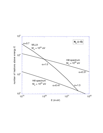
Figure 2: Left: Differential energy spectrum (multiplied by $E^{2}$) of the secondary photons in a top-down jet, for various models (adapted from Bhattacharjee and Sigl [3]). Right: Integrated energy spectrum giving the total number of photons above energy $E$ in the jet, for the same models. The slope of the approximate power-law (spectral index $\alpha$) is indicated.

Concerning the jet particle multiplicity, we show on Fig. 2a the typical spectrum (multiplied by $E^{2}$) obtained with a modified leading-log approximation (MLLA) model, assuming that the X-particle mass is at the GUT scale, i.e. $M_{\mathrm{X}}\simeq 10^{25}~{}\mathrm{eV/c}^{2}$ (adapted from [3]). Also shown are the hadron jet spectra obtained with the Hill formula for X-particle masses of $10^{25}~{}\mathrm{eV/c}^{2}$ and $10^{28}~{}\mathrm{eV/c}^{2}$. In all cases, it is expected that most of the jet energy be distributed among UHE particles. Following some previous works, we consider here MLLA spectra, which are found not to have a simple power-law behavior in the energy range of interest, namely around $10^{20}$ eV, and to be steeper than often quoted for top-down scenarios – as would result from Hill’s formula. It has been argued, however, that the MLLA spectra do not reproduce faithfully the fragmentation spectrum in the last energy decade or so, i.e. at energies close to the X-particle mass [10]. In this study, we shall only consider X-particle masses above $10^{23}$ eV, so that the UHECRs of interest have energies well below $m_{\mathrm{X}}$. The MLLA spectral shape may thus represent a reasonable approximation of the fragmentation spectrum around $10^{20}$ eV. The normalization is probably more problematic, however, because it depends largely on the amount of energy carried out by the rarest, most energetic particles in the jet. Any other normalization than adopted below will lead to characteristic timescales for multiple event detection that scale according to Eq. (11), as $N_{\gamma}^{-1/2}$.

In Fig. 2b, we have plotted the integrated hadron jet spectrum corresponding to the same cases as in Fig.2a. If one tries to approximate the spectrum by a power-law $\mathrm{d}N/\mathrm{d}E\propto E^{-x}$ (i.e. $N(\geq E)\propto E^{-\alpha}$, with $\alpha=x-1$), the logarithmic slope is approximately constant for the Hill spectra, while it goes from 1.7 to 2.3 in the energy range of interest, with a value of $\sim 2$ at $10^{20}$ eV, for the MLLA spectrum. In our ‘toy jet model’, we shall assume a mean hadron spectrum in $E^{-2}$ between $E_{\mathrm{inf}}=10^{19}$ eV and $E_{\mathrm{sup}}=10^{22}$ eV: $N(E)=\eta E_{\mathrm{jet}}/E^{2}$, where $\eta$ is a numerical constant, so that $N(\geq E)=\eta(E_{\mathrm{jet}}/E-1)\simeq\eta E_{\mathrm{jet}}/E$. A fit of the MLLA spectrum in Fig. 2 gives $\eta\simeq 0.10$, so that about 70% of the jet energy is in particles with energies above $10^{19}$ eV. Only about one third of this energy, however, will be imparted to the photons, assuming that the total jet energy is divided up evenly into the three types of pions ($\pi^{0}$, $\pi^{+}$ and $\pi^{-}$), of which only the neutral ones decay into photons, and neglecting in a first approximation the contribution of nucleons.

In conclusion, we shall adopt for the UHE photons the above $E^{-2}$ spectrum with a value of $\eta=0.033$. We shall also extrapolate the same spectrum to hadron jets generated by X-particles of lower mass, but with $E_{\mathrm{jet}}$, $E_{\mathrm{inf}}$ and $E_{\mathrm{sup}}$ scaled linearly. This will allow us to explore UHECR progenitors with masses down to $10^{23}$ eV. Assuming that the X particle decay events lead to the formation of two jets, so that $E_{\mathrm{jet}}=M_{\mathrm{X}}c^{2}/2$, one finally obtains the following approximate formula (only valid between $E_{\mathrm{inf}}$ and $E_{\mathrm{sup}}$):

$$N_{\gamma}(\geq E)\simeq 1.7\times 10^{3}\left(\frac{E}{10^{20}\,\mathrm{eV}}\right)^{-1}\left(\frac{M_{\mathrm{X}}c^{2}}{10^{25}\,\mathrm{eV}}\right).$$ (12)

4.2 The jet opening angle

Coming now to the question of the jet opening angle, let us first note that a naive line of reasoning based on the Lorentz factor collimation effect cannot apply here. One might have been tempted to derive $\theta_{\mathrm{jet}}$ by claiming that an isotropic distribution of the jet particles in the rest frame of the parent quark would translate in the Galactic frame into a collimated distribution within a cone of opening angle $1/\Gamma_{q}$, where $\Gamma_{q}$ is the quark’s Lorentz factor. However, such a collimation only applies to the decay products of real particles, not virtual ones. In the case considered here, the parent X-particle is at rest in the Galactic frame, and the jet particles are created out of the extremely intense field represented by a quark/anti-quark pair moving apart, not by the ‘decay’ of one of its members. In a QCD jet, as it turns out, the hadronization process allows in principle large emission angles, i.e. large values of the particle momentum in a direction perpendicular to the jet axis, $p_{\perp}$.

A standard angular distribution is given by the following logarithmic law:

$$\frac{\mathrm{d}N}{\mathrm{d}p_{\perp}^{2}}\simeq\frac{1}{p_{\perp}^{2}+\Lambda_{QCD}^{2}},$$ (13)

where the regularisation momentum, $\Lambda_{QCD}$, is a typical effective QCD scale, of the order of 300 MeV. Using this expression, and the fact that the emission angle of a particle is given by $\theta(p_{\perp})\simeq p_{\perp}/p_{\parallel}\simeq p_{\perp}c/E$, one finds that about 10% of the jet particles are found with $p_{\perp}<30\Lambda_{QCD}$, i.e. within $\theta_{\mathrm{jet}}\simeq 9\times 10^{-11}(E/10^{20}\,\mathrm{eV})^{-1}$, with only a weak dependence on the X-particle mass (logarithmic in the large quantity $M_{\mathrm{X}}c^{2}/\Lambda_{\mathrm{QCD}}$). This represents a considerably weaker collimation than what would have been obtained from a Lorentz factor argument applied to a progenitor real quark, giving the opening angle $\theta_{\mathrm{jet}}\simeq 1/\Gamma_{\mathrm{q}}\simeq 3\times 10^{-14}(M_{\mathrm{X}}c^{2}/10^{25}\,\mathrm{eV})^{-1}$.

In practice, however, the energy is found to be better collimated than the multiplicity in QCD jets [13], and one expects the highest energy particles (which we are interested in) to be much better collimated than obtained from Eq. (13). In other words, the largest perpendicular momenta in the jet distribution are attributed statistically more often to the lower-energy particles. Moreover, this behaviour is found to be amplified as the jet energy increases. This is important for our concern, because we are interested only in the particles in the last few decades of the energy range (above a few $10^{19}$ eV), and not in all the (much more numerous) particles between this energy and the GeV range, which may fill a cone with a larger opening angle, but which shall not be detected as UHECRs anyway.

Extrapolating the semi-empirical theory available at CERN energies towards the ultra-high energies of interest, one finds that for a quark jet, about 50% of the jet energy is found within $\theta_{\mathrm{UHE}}\sim 2\times 10^{-12}$ radians of the jet axis (Dokshitzer, private communication). Considering this number as well as that obtained from Eq. (13), we shall arbitrarily adopt the following, hopefully conservative value for the UHECR jet opening angle:

$$\theta_{\mathrm{jet}}\simeq 2\times 10^{-11}.$$ (14)

The above estimates are admittedly arguable, and cannot be expected to hold for all models, but they may represent a reasonable description of the jets in the energy range of interest. Any other assumptions about $\mathrm{d}N_{\mathrm{gamma}}/\mathrm{d}E$ and $\theta_{\mathrm{jet}}$ (e.g. motivated by a detailed study of a particular top-down model) can be used in the following, in a straightforward replacement of ours.

4.3 Observability of multiple events with the PAO and EUSO

Let us now evaluate the characteristic timescale of double event observation, $\tau_{2}$, by replacing the various model parameters by their numerical values in Eq. (11). The flux of top-down UHECRs above the detector’s threshold energy, $\Phi^{\mathrm{td}}_{\geq E_{\mathrm{th}}}$, is obtained consistently with the assumed hadronization spectrum: we normalize the $E^{-2}$ spectrum to the quoted value of $3\times 10^{-40}\,\mathrm{cm}^{-2}\mathrm{s}^{-1}\mathrm{sr}^{-1}\mathrm{eV}^{-1}$ at $10^{20}$ eV, i.e. we assume that all the UHECRs at $10^{20}$ eV have a top-down origin (and only a fraction of them below that energy). One thus obtains:

$$\Phi_{\mathrm{CR}}(\geq E)\simeq(10^{-2}\,\mathrm{km}^{-2}\mathrm{yr}^{-1}\mathrm{sr}^{-1})\times\left(\frac{E}{10^{20}\,\mathrm{ev}}\right)^{-1},$$ (15)

from which it follows:

$$\tau_{2}\simeq(2.1\,\,\mathrm{yr})\times\left(\frac{S_{\mathrm{d}}}{3000\,\mathrm{km}^{2}}\right)^{-3/2}\left(\frac{\delta}{100\%}\right)^{-1}\left(\frac{E_{\mathrm{th}}}{10^{19}\,\mathrm{eV}}\right)^{3/2}\left(\frac{M_{\mathrm{X}}}{10^{25}\,\mathrm{eV}}\right)^{-1/2}.$$ (16)

In the case of the next generation UHECR observatories, the detection surface on the ground will be $3000\,\mathrm{km}^{2}$ for the PAO (one site), and $1.5\times 10^{5}\,\mathrm{km}^{2}$ for EUSO. The detector’s duty cycles are respectively 100% and 14%, and the energy thresholds are $10^{19}$ eV for the PAO and $5\times 10^{19}$ eV for EUSO. With these number, one finds, for an X-particle at the GUT scale ($M_{\mathrm{X}}=10^{25}\,\mathrm{eV}$):

$$\tau_{2}(\mathrm{PAO})=2.1\,\mathrm{yr}\quad\mathrm{and}\quad\tau_{2}(\mathrm{EUSO})=0.48\,\mathrm{yr},$$ (17)

which are smaller than the observatories’ lifetimes (15 and 3 years, respectively). The timescales for triple, quadruple and quintuple event detections are respectively 2 times, 2.67 and 3.2 times larger, as follows from Eq. (10).

As indicated above, these timescales scale with the X-particle mass as $M_{\mathrm{X}}^{-1/2}$, and with the actual number of UHE photons within the jets as $N_{\gamma}^{1/2}$. Even a drastic decrease in the photon multiplicity in the jet by an order of magnitude would only increase the lifetimes by a factor $\sqrt{1}0$ and keep the double event detection timescales smaller than the lifetime of each experiments. The sensitivity to $\theta_{\mathrm{jet}}$ is linear, however, and jet models with much larger opening angles than assumed here would make double event detection more problematic. We should also note that decay modes into more than two jets would lead to smaller photon multiplicities, so that $\tau_{2}$ would also scale as $N_{\mathrm{jet}}^{1/2}$.

5 Strong upper limit on the double detection timescale

Considering the above uncertainties, we shall now derive a model-independent limit for the detection of double events, based on the fact that every UHE photon in a top-down model comes from the decay of a neutral pion, and is therefore accompanied by a second photon within a very small angle, due to relativistic beaming. For a photon pair at $10^{20}$ eV, say, the parent pion Lorentz factor is $\Gamma_{\pi}=2E/m_{\pi}c^{2}\simeq 1.4\times 10^{12}$, so that the opening angle of this minimal, two-particle jet is $\theta_{\mathrm{jet}}\simeq 1/\Gamma_{\pi}\simeq 7\times 10^{-13}$. Using the source distance distribution, Eq. (3), and averaging over the decay angle in the pion rest frame, one finds the probability distribution of the distance $d$ between the two photons of a pair corresponding to a random UHECR event:

$$p(d)=\frac{\pi}{8}\frac{\Gamma_{\pi}}{D_{0}}\quad\mathrm{for}\quad d\ll D_{0}/\Gamma_{\pi}.$$ (18)

This allows us to estimate the probability that a detected UHE photon be accompanied by a second one within the range of the detector (of radius $R_{\mathrm{d}}$):

$$\mathcal{P}_{2}\simeq\frac{\pi}{16}\frac{\Gamma_{\pi}\left<R_{\mathrm{d}}\right>_{\perp}}{D_{0}}\simeq 7.8\times 10^{-5}\left(\frac{E}{10^{20}\,\mathrm{eV}}\right)\left(\frac{R_{\mathrm{d}}}{200\,\mathrm{km}}\right),$$ (19)

From this, one can derive the minimum characteristic timescale for double event detection (independent of both $\theta_{\mathrm{jet}}$ and $N_{\gamma}$):

$$\tau_{2}^{\mathrm{min}}\simeq\frac{1}{\dot{N}_{\mathrm{evt}}\mathcal{P}_{2}}\simeq\frac{1}{\Phi^{\mathrm{td}}(\geq E)\pi^{2}R_{\mathrm{d}}^{2}\delta\,\mathcal{P}_{2}}\simeq 23\,\,\mathrm{yr}\left(\frac{\delta}{14\%}\right)\left(\frac{R_{\mathrm{d}}}{200\,\mathrm{km}}\right)^{-3}.$$ (20)

While this timescale may seem prohibitively long (17 years for the EUSO detector, of radius $\sim 220$ km), one should note the cubic dependence in $R_{\mathrm{d}}$: a detector only two times larger (i.e. on an orbit two times higher) would detect double events from the minimal top-down jets on a timescale slightly above 2 years. This model-independent upper limit may give confidence that multiple event detection should indeed be possible, if the UHECRs are produced in Galactic top-down jets containing not just two photons from an isolated $\pi^{0}$ decay, but thousands of UHE photons.

6 Conclusion

In this paper, we have studied the possibility of observing multiple UHECR events from Galactic hadron jets, resulting from the decay of supermassive X-particles in the Halo. We have shown that, under reasonable assumptions about the jet properties, the next generation UHECR detectors should be able to detect a few double events, and possibly one or two triple and quadruple events, provided the UHE flux is dominated by top-down sources at about $10^{20}$ eV, and the mass of the X-particle progenitor is around the GUT scale.

The main uncertainties in our calculations come from the jet model. Our assumptions about the photon spectrum, the jet multiplicity and the jet opening angle can only be considered as rough estimates, and other X-particle model may lead to different values. Nevertheless, we have derived a general framework for the study of multiple events probability, and given a way to calculate the relevant detection timescales for any X-particle model, once its physical parameters are specified. In particular, we have shown that the timescale $\tau_{2}$ is proportional to the jet opening angle, and inversely proportional to the square root of the photon multiplicity in the jets.

Considering the jet uncertainties, we have also derived the double event detection timescale for the worst possible case: a two-particle jet consisting of the two photons produced by the decay of a neutral pion, as must be found in any Galactic hadron jet, whatever the model considered. This gives an upper limit on $\tau_{2}$ which would reduce to $\sim 2$ years for a detector twice as large as EUSO. Note that this is also independent of the X-particle mass, contrary to the timescales obtained by taking into account all the particles inside the jet. Note also that we have assumed homogeneously distributed photons inside the jets. In the case of a clumpy distribution, the probability of observing a multiple event can only be higher than what we have obtained here, because the photon density close to an arbitrary photon would then be higher (on average) than the mean photon density in the jet.

Besides this new test of Galactic top-down models, three other observational signatures have already been proposed. First, top-down scenarios predict that photons should be the dominant component among UHECRs above $10^{20}$ eV. As we have seen, this is very important for our study, because charged particles of even ultra-high rigidity would be slightly deflected in the Galactic magnetic fields and lose the almost perfect collimation which multiple event require. Second, the dipole anisotropy due to the off-centered position of the Earth should eventually show up in the data, although this indirect evidence might not be fully discriminatory, since at least one bottom-up model has been proposed with the same characteristics [14]. Finally, the UHECR energy spectrum should be characteristic of a hadronic fragmentation process, which may be quite different from the power laws usually expected from astrophysical acceleration processes. However, the exact shape of the spectrum is still hard to predict precisely in any of the top-down or bottom-up models, and it is not clear whether a measurement with reasonable error bars over two decades in energy at most ($10^{19}$ to $10^{21}$ eV, say) can lead to definitive conclusions.

By contrast, the detection of (were it only) one multiple event would provide a clear, direct evidence that a top-down scenario is involved, because it is highly improbable that two independent, bottom-up UHECRs arrive exactly at the same time from exactly the same direction. In this respect, we should recall that a previous study excluded (or more precisely found very improbable) the possibility that a heavy nucleus be photodisintegrated by the solar radiation field and give rise to a pair of showers from the lighter, daughter nuclei [15] (besides, such a pair would be perfectly correlated with the Sun’s position).

As shown above, the ideal detector to implement such a test and detect multiple events from Galactic-size hadron jets is a detector of very large acceptance, but not necessarily good angular and energy resolutions, which is usually one of the main challenges for UHECR detectors. One might therefore think about the interest of devising a detector made of a series of atmospheric fluorescence telescopes covering a huge surface on Earth, but with poor angular and energy resolutions in order to keep it economical.

Finally, we note that while the jet parameters are a major cause of uncertainty in the calculation of multiple events detection timescales, this very fact may offer a possibility to constrain them (if the top-down origin of UHECRs were to be attested by this or another way). This may represent a unique opportunity to study the hadronization processes at energies many orders of magnitude above what can be reached in terrestrial accelerators.

7 Acknowledgements

I wish to thank warmly Yuri Dokshitzer and Michel Fontannaz for enlightening discussions and comments about QCD processes, jet formation and hadronization.

Appendix A Appendix

In this appendix, we derive the general expression of the probability of detecting a multiple event as a function of the total number of UHECRs detected, which we shall note here $N$ instead of $N_{evt}$, for convenience. The probability of an event of multiplicity $m\geq n$ will be denoted by $\mathcal{P}_{\geq n}(N)$, and we shall prove that it can be written as in Eq. (5):

$$\mathcal{P}_{\geq n}(N)=1-e^{-\frac{N}{N_{n}}},$$ (21)

with the following values of the constants $N_{n}$:

$$N_{2}=\frac{1}{\sqrt{\pi}}\mu_{0}^{-1/2},\quad\mathrm{and}\quad N_{n+2}=\frac{2n}{2n-1}N_{n+1},$$ (22)

which hold for small values of $n$, compared to the jet multiplicity $n\ll N_{\gamma}$.

Each useful X-particle decay event (i.e. giving rise to the detection of at least one UHECR), can be indexed by an integer $k$ ($1\leq k\leq N$), and is characterized by its distance, $D_{k}$, to the detector. Its corresponding potential multiplicity is given by Eq. (4): $\mu_{k}=\mu_{0}D_{0}^{2}/D_{k}^{2}$. The statistics of multiple events detection will therefore be determined by the statistics of the source distances, Eq. (3): $p(D)=1/D_{0}$, for $0\leq D\leq D_{0}$. Combining both expressions, we find the probability distribution of the random variable $\mu$:

$$p(\mu)=p(D)\left|\frac{\mathrm{d}D}{\mathrm{d}\mu}\right|=\frac{1}{2}\mu_{0}^{1/2}\mu^{-3/2}\quad\quad(\mu_{0}\leq\mu\leq\infty).$$ (23)

We shall first establish that, for one particular (useful) X-particle decay event with potential multiplicity $\mu$, the probability that it is not an event with actual multiplicity $m\geq n$ writes, for $n\ll N_{\gamma}$:

$$\tilde{\mathcal{P}}(m\geq n,\mu)=(1+\mu+\frac{\mu^{2}}{2!}+\ldots+\frac{\mu^{n-2}}{(n-2)!})\,e^{-\mu}.$$ (24)

We proceed by recursion. For $n=2$, the property reads $\tilde{\mathcal{P}}(m\geq 2,\mu)=1-\mathcal{P}(m\geq 2,\mu)=e^{-\mu}$, and has been obtained in Sect. 2. Then:

$$\tilde{\mathcal{P}}(m\geq n+1,\mu)\equiv 1-\mathcal{P}(m\geq n+1,\mu)=\tilde{\mathcal{P}}(m\geq n,\mu)+\mathcal{P}(n,\mu),$$ (25)

where $\mathcal{P}(n,\mu)$ was given in Eq. (2), and develops into:

$$\mathcal{P}(n,\mu)=\frac{\mu^{n-1}}{(n-1)!}\frac{(N_{\gamma}-1)\ldots(N_{\gamma}-(n-1))}{N_{\gamma}^{n-1}}\frac{\left(1-\frac{\mu}{N_{\gamma}}\right)^{N_{\gamma}}}{\left(1-\frac{\mu}{N_{\gamma}}\right)^{m}},$$ (26)

and thus, for $n\ll N_{\gamma}$:

$$\mathcal{P}(n,\mu)\simeq\frac{\mu^{n-1}}{(n-1)!}e^{-\mu},$$ (27)

which completes the proof.

Now we consider the $N$ events together, and note that the ‘non-detection probabilities’, $\tilde{\mathcal{P}}(m\geq n)$, simply multiply:

$$\tilde{\mathcal{P}}(m\geq n,\{\mu_{k}\})=\prod_{k=1}^{N}\tilde{\mathcal{P}}(m\geq n,\mu_{k}).$$ (28)

Now the global multiple event probability, $\mathcal{P}_{\geq n}(N)$, is the average value of $\mathcal{P}(m\geq n,\{\mu_{k}\})=1-\tilde{\mathcal{P}}(m\geq n,\{\mu_{k}\})$:

$$\begin{split}\mathcal{P}_{\geq n}(N)&=\left<1-\prod_{k=1}^{N}\tilde{\mathcal{P}}(m\geq n,\mu_{k})\right>\\ &=1-\left<\prod_{k=1}^{N}[(1+\mu_{k}+\ldots+\frac{\mu_{k}^{n-2}}{(n-2)!})\,e^{-\mu_{k}}]\right>\\ &=1-\left<\tilde{\mathcal{P}}(m\geq n,\mu)\right>^{N},\end{split}$$ (29)

where the last equality follows from the statistical independence of the various $\mu_{k}$.

This is indeed of the form announced in Eq. (21), provided that we define the characteristic numbers $N_{n}$ by:

$$N_{n}\equiv\frac{-1}{\ln\left<\tilde{\mathcal{P}}(m\geq n,\mu)\right>}.$$ (30)

We thus have to calculate the average value of $\tilde{\mathcal{P}}(m\geq n,\mu)$:

$$\left<\tilde{\mathcal{P}}(m\geq n,\mu)\right>=\left<\tilde{\mathcal{P}}(m\geq n-1,\mu)\right>+\frac{1}{(n-2)!}\left<\mu^{n-2}e^{-\mu}\right>,$$ (31)

where, with the probability law of Eq. (23):

$$\left<\mu^{n-2}e^{-\mu}\right>=\int_{\mu_{0}}^{\infty}\mu^{n-2}e^{-\mu}p(\mu)\mathrm{d}\mu=\frac{\mu_{0}^{1/2}}{2}\int_{\mu_{0}}^{\infty}\mu^{n-2-3/2}e^{-\mu}\mathrm{d}\mu.$$ (32)

Integrating by parts, one finds:

$$\left<\mu^{n-2}e^{-\mu}\right>=\tfrac{1}{2}\mu_{0}^{n-3}e^{-\mu_{0}}+(n-2-\tfrac{3}{2})\left<\mu^{n-3}e^{-\mu}\right>.$$ (33)

We shall now use the fact that $\mu_{0}\ll 1$ and limit the calculations to the lowest order (first order in $\mu_{0}^{1/2}$). We can thus drop the first term in the right-hand side of the above equation, as long as $n\geq 4$, and rewrite it as:

$$\left<\mu^{n-2}e^{-\mu}\right>=(n-2-\tfrac{3}{2})\left<\mu^{n-3}e^{-\mu}\right>,\quad(n\geq 4),$$ (34)

from where it follows, using Eq. (31) and writing $I_{n}\equiv\left<\tilde{\mathcal{P}}(m\geq n,\mu)\right>$ for simplicity, that

$$I_{n}-I_{n-1}=\frac{n-2-\tfrac{3}{2}}{n-2}(I_{n-1}-I_{n-2}),\quad(n\geq 4).$$ (35)

This will allow us to calculate $I_{n}$ for all $n\geq 4$, once we know $I_{2}$ and $I_{3}$. Starting with $I_{2}=\int_{\mu_{0}}^{\infty}e^{-\mu}p(\mu)\mathrm{d}\mu$ and integrating by parts, one finds:

$$I_{2}=e^{-\mu_{0}}-\mu_{0}^{1/2}\int_{\mu_{0}^{1/2}}^{\infty}\mu^{-1/2}e^{-\mu}\mathrm{d}\mu,$$ (36)

and then, by changing the variable to $u=\mu^{1/2}$:

$$I_{2}=e^{-\mu_{0}}-2\mu_{0}^{1/2}\int_{\mu_{0}^{1/2}}^{\infty}e^{-u^{2}}\mathrm{d}u\simeq e^{-\mu_{0}}-\sqrt{\pi}\mu_{0}^{1/2},$$ (37)

where we have used $\mu_{0}\ll 1$ in the gaussian integral. Developing to first order in $\mu_{0}^{1/2}$, we thus obtain:

$$I_{2}\simeq 1-\sqrt{\pi}\mu_{0}^{1/2},$$ (38)

and the first characteristic event number (for double event detection):

$$N_{2}=\frac{-1}{\ln I_{2}}\simeq\frac{1}{\sqrt{\pi}}\mu_{0}^{-1/2},$$ (39)

as announced in (22).

Coming now to $I_{3}=\int_{\mu_{0}}^{\infty}(1+\mu)e^{-\mu}p(\mu)\mathrm{d}\mu$, we have

$$I_{3}=I_{2}+\int_{\mu_{0}}^{\infty}\mu e^{-\mu}p(\mu)\mathrm{d}\mu=I_{2}+\frac{1}{2}\mu_{0}^{1/2}\int_{\mu_{0}^{1/2}}^{\infty}\mu^{-1/2}e^{-\mu}\mathrm{d}\mu,$$ (40)

where we can replace the last term, using Eq. (36):

$$I_{3}=\frac{1}{2}(I_{2}+e^{-\mu_{0}})\simeq 1-\frac{\sqrt{\pi}\mu_{0}^{1/2}}{2}.$$ (41)

This allows us to write the characteristic number of events for the detection of triple events, $N_{3}=-1/\ln I_{3}$, as:

$$N_{3}=\frac{2}{\sqrt{\pi}}\mu_{0}^{-1/2}=2\times N_{2}.$$ (42)

From (38) and (41), we find

$$I_{3}-I_{2}=\frac{\sqrt{\pi}\mu_{0}^{1/2}}{2},$$ (43)

which we can insert into (35) to obtain:

$$I_{4}=I_{3}+\frac{2-\frac{3}{2}}{2}(I_{3}-I_{2})\simeq 1-\frac{3}{8}\sqrt{\pi}\mu_{0}^{1/2},$$ (44)

and thus

$$N_{4}=\frac{8}{3}\frac{\mu_{0}^{-1/2}}{\sqrt{\pi}}=\frac{4}{3}\times N_{3}.$$ (45)

More generally, we can show that, at the first order in $\mu_{0}^{1/2}$,

$$I_{n}=1-\alpha_{n}\sqrt{\pi}\mu_{0}^{1/2},\quad\mathrm{with}\quad\alpha_{n}=\alpha_{n-1}\frac{2(n-2)-1}{2(n-2)}.$$ (46)

We have already found that this is true for $n=2$ and $n=3$. If we now assume that it is true for $n-2$ and $n-1$, we can use Eq. (35) to calculate $I_{n}$:

$$\begin{split}I_{n}&=I_{n-1}+\frac{2(n-2)-3}{2(n-2)}(I_{n-1}-I_{n-2})\\ &=1-\sqrt{\pi}\mu_{0}^{1/2}\alpha_{n-1}-\frac{2n-7}{2n-4}(\alpha_{n-1}-\alpha_{n-2})\sqrt{\pi}\mu_{0}^{1/2}\\ &=1-\sqrt{\pi}\mu_{0}^{1/2}\alpha_{n-1}\left[1+\frac{2n-7}{2n-4}-\frac{2n-7}{2n-4}\frac{2(n-3)}{2(n-3)-1}\right]\\ &=1-\sqrt{\pi}\mu_{0}^{1/2}\alpha_{n-1}\frac{2(n-2)}{2(n-2)-1},\end{split}$$ (47)

which is indeed the recursion relation (46).

The characteristic number of events for a multiplicity larger than $n$ is thus finally:

$$N_{n}=\frac{-1}{\ln I_{n}}=\frac{1}{\alpha_{n}}\frac{\mu_{0}^{1/2}}{\sqrt{\pi}},$$ (48)

and the recursion relation (22) simply follows from that in (46). QED.

References

- [1] H. Ayashida et al., Phys. ReV. Lett., 73, 3491 (1994). D. J. Bird et al, Astrophys. J., 441, 144 (1995).
- [2] K. Greisen, Phys. Rev. Lett. 16, 748 (1966). G. T. Zatsepin and V. A. Kuzmin, Pis’ma Zh. Eksp. Teor. Fiz. 4, 114 (1966).
- [3] for a general review on UHECRs, see e.g., P. Bhattacharjee and G. Sigl, Phys. Reports, 327, 109 (2000), or the recent book Physics and Astrophysics of Ultra-High Energy Cosmic Rays M. Lemoine and G. Sigl, Eds., Springer-Verlag, Berlin (2001), and references therein.
- [4] S. van den Bergh, PASP, 108, 1091 (1996).
- [5] G. A. Medina Tanco and A. A. Watson, Astropart. Phys., 12, 25 (1999).
- [6] V. Berezinsky, M. Kachelrieß and A. Vilenkin, Phys. Rev. Lett., 79, 4302 (1997). M. Birker and S. Sarkar, Astropart. Phys., 9, 297 (1998). S. Sarkar and R. Toldra, Nucl.Phys. B621, 495 (2002).
- [7] T. Dova et al., in Proc. of 27th ICRC, Hamburg, 2, 699 (2001). R. Cester et al., in Proc. of 27th ICRC, Hamburg, 2, 711 (2001). See also the web site at http://www.auger.org/
- [8] See the web site at http://www.ifcai.pa.cnr.it/ EUSO/
- [9] J. Linsley et al., in Proc. of 25th ICRC, Durban, 5, 381 (1997). See also the web site at http://owl.uah.edu/
- [10] S. Sarkar, in ‘COSMO-99, Third Intern. Workshop on Particle Physics and the Early Universe’, p. 77 (hep-ph/0005256).
- [11] J. A. R. Caldwell and J. P. Ostriker, Astrophys. J., 251, 61 (1981)
- [12] J. F. Navarro, C. S. Frenk and S. D. M. White, Astrophys. J., 462, 563 (1996).
- [13] Yu. L. Dokshitzer, V. A. Khoze, A. H. Mueller and S. I. Troyan, Basics of Perturbative QCD, ed. J. Tran Thanh Van, Editions Frontières, Saclay (1991).
- [14] A. Dar and R. Plaga, Astron. & Astroph., 349, 259 (1999)
- [15] N. M. Gerasimova and G. T. Zatsepin, JETP, 11, 899 (1960). G. A. Medina Tanco and A. A. Watson, Astropart. Phys., 10, 157 (1999).