CHANDRA Observations of QSO 2237+0305

Abstract

We present the observations of the gravitationally lensed system QSO 2237+0305 (Einstein Cross) performed with the Advanced CCD Imaging Spectrometer (ACIS) onboard the Chandra X-ray Observatory on 2000 September 6, and on 2001 December 8 for 30.3 ks and 9.5 ks, respectively. Imaging analysis resolves the four X-ray images of the Einstein Cross. A possible fifth image is detected; however, the poor signal-to-noise ratio of this image combined with contamination produced by a nearby brighter image make this detection less certain. We investigate possible origins of the additional image. Fits to the combined spectrum of all images of the Einstein Cross assuming a simple power law with Galactic and intervening absorption at the lensing galaxy yields a photon index of $1.90^{+0.05}_{-0.05}$ consistent with the range of $\Gamma$ measured for large samples of radio-quiet quasars. For the first Chandra observation of the Einstein Cross this spectral model yields a 0.4–8.0 keV X-ray flux of $4.6\times 10^{-13}\hbox{erg~{}cm${}^{-2}$~{}s${}^{-1}$}$ and a 0.4–8.0 keV lensed luminosity of $1.0\times 10^{46}\hbox{erg~{}s${}^{-1}$}$. The source exhibits variability both over long and short time scales. The X-ray flux has dropped by 20% between the two observations, and the Kolmogorov-Smirnov test showed that image A is variable at the 97% confidence level within the first observation. Furthermore, a possible time-delay of $2.7^{+0.5}_{-0.9}$ hours between images A and B with image A leading is detected in the first Chandra observation. The X-ray flux ratios of the images are consistent with the optical flux ratios which are affected by microlensing suggesting that the X-ray emission is also microlensed. A comparison between our measured column densities and those inferred from extinction measurements suggests a higher dust-to-gas ratio in the lensing galaxy than the average value of our Galaxy. Finally, we report the detection at the 99.99% confidence level of a broad emission feature near the redshifted energy of the Fe K$\alpha$ line in only the spectrum of image A. The rest frame energy, width, and equivalent width of this feature are $E_{line}$ = $5.7_{-0.3}^{+0.2}$ keV, $\sigma_{line}$ = $0.87_{-0.15}^{+0.30}$ keV, and $EW=1200^{+300}_{-200}$ eV, respectively.

1 Introduction

QSO 2237+0305 was discovered by Huchra et al. (1985) as part of the Center for Astrophysics galaxy redshift survey. Four images have been resolved (Schneider et al., 1988; Yee, 1988) from this lens system. The quasar is at a redshift of $z_{s}=1.695$ and the lensing galaxy is at a redshift of $z_{l}=0.0395$. Microlensing induced by stars in the lens galaxy was proposed for this system shortly after its discovery (Kayser, Refsdal, & Stabell, 1986; Kent & Falco, 1988; Schneider et al., 1988; Kayser & Refsdal, 1989), and was first confirmed by Irwin et al. (1989). Microlensing in QSO 2237+0305 has been firmly established with extensive monitoring of this system over several years (Racine, 1992; Østensen et al., 1996; Wo$\acute{\rm{z}}$niak et al., 2000a, b). The presence of both macrolensing and microlensing in the Einstein Cross and the proximity of the lensing galaxy, an order of magnitude closer than other lensing galaxies, make it a unique laboratory to explore the structure of the different emission regions in the source quasar, and the properties of the lensing galaxy as well.

During the past decades, major progress has been made in understanding the physical processes associated with Active Galactic Nuclei (AGN); however, it is beyond the capabilities of current telescopes to resolve directly the central parts of AGNs. Observations of quasar microlensing events provide a means of exploring the structure of AGNs. Multi-wavelength studies of QSO 2237+0305 (Falco et al., 1996; Mediavilla et al., 1998; Agol, Jones, & Blaes, 2000) demonstrate that the flux ratios of the images are different in different bands, in particular, between the radio, C iii], mid-infrared, and optical. The differences of flux ratios in different wavelength bands has been interpreted as the result of microlensing. Emission regions with a size significantly less than the Einstein radius of the microlens in the source plane will be significantly magnified, whereas, emission regions with a size significantly larger than the Einstein radius will not be affected by microlensing. Studies of QSO 2237+0305 indicate that the radio and mid-infrared emission regions are larger than the Einstein radius, whereas, the optical emission regions are smaller than the Einstein radius. The C iii] emission regions also extend beyond the Einstein radius but are less extended than the radio and mid-infrared regions. The analysis of light-curves of microlensing events can also constrain the source size of individual emission regions, especially in a high magnification event (HME) that may occur during a caustic crossing. Yonehara (2001) analyzed the light-curves of QSO 2237+0305 and estimated a source size of less than 2000 AU for the optical emission region in QSO 2237+0305. It is desirable to study the X-ray emission of a microlensed quasar since the X-rays are thought to originate from the inner most region of the accretion disc. The X-ray light-curves of the images and the profile of the Fe K$\alpha$ line during a microlensing event, especially from a HME, could constrain the X-ray emission region and possibly yield information about the mass and spin of the central black hole (Yonehara et al., 1998; Agol & Krolik, 1999; Popovi$\acute{\rm{c}}$ et al., 2002). Recently, a microlensing event in X-rays was observed by Chartas et al. (2002) in MG J0414+0534, where an enhancement of the equivalent width of the Fe K$\alpha$ line was observed in only one of the images.

As mentioned earlier the proximity of the lensing galaxy of 2237+0305 has facilitated its detailed study in several wave bands. In particular, Yee (1988) detected a $g-i$ color difference between different image components which indicates differential extinction. The extinction curve for the lensing galaxy was measured by Nadeau et al. (1991). Foltz et al. (1992) measured the central velocity dispersion of the barred spiral galaxy 2237+0305 to be $215\pm 30~{}\hbox{km~{}s${}^{-1}$}$. Modeling of the lens system has also provided estimates of the mass distributions of the lensing galaxy. In particular, Schmidt, Webster, & Lewis (1998) studied the contribution of the galaxy bar to the lens potential and found a bar-mass of about $7.5\times 10^{8}\hbox{${M}_{\odot}$}$.

QSO 2237+0305 was first detected in X-rays with ROSAT by Wambsganss et al. (1999); however, due to the low spatial resolution of ROSAT, the individual images were not resolved. To obtain spatially resolved X-ray spectra from the individual images we performed Chandra observations of QSO 2237+0305. Here, we present the results of these observations. We use $H_{0}$ = 65 km s^-1 Mpc^-1, $\Omega_{m}=0.3$, and $\Omega_{\Lambda}$ = 0.7, unless mentioned otherwise.

2 Observations and Data Reduction

QSO 2237+0305 was observed with ACIS (Garmire et al., 2002) onboard the Chandra X-ray Observatory for $\sim 30.3$ ks and $\sim 9.5$ ks on 2000 September 6, and 2001 December 8, respectively. The data were taken continuously with no interruptions within each observation. QSO 2237+0305 was placed at the aim point of the ACIS-S array which is on the back-illuminated S3 chip. The data were reduced with the CIAO 2.2 software tools provided by the Chandra X-ray Center (CXC). We improved the image quality of the data by removing the pixel randomization applied to the event positions in the CXC processing and by applying a subpixel resolution technique (Tsunemi et al., 2001; Mori et al., 2001). In the first and second observations of QSO 2237+0305  we detected background flares with durations of $\sim 10$ ks and $\sim 0.2$ ks, respectively. We did not remove events collected during the background flares in either of the two observations because even at the peak of the flares, the backgrounds only contribute by about 0.3% and 1% of the counts of QSO 2237+0305 for the first and second observation, respectively. In the data analysis, only events with standard ASCA grades of 0, 2, 3, 4, and 6 were used.

3 Photometry and Astrometry

Totals of 2632 and 607 source events were detected from circles centered on the centroids of the sources with radii of 3^′′ and within the 0.2-10 keV energy band during the first and second observations of QSO 2237+0305, respectively. We applied a point spread function (PSF) fitting method to estimate the X-ray count rates of individual images due to the closeness of the individual images. We modeled the Chandra images of A, B , C and D with PSFs generated by the simulation tool MARX (Wise et al., 1997). The X-ray event locations were binned with a bin-size of 0${}^{\prime\prime}\!\!.$0246. The simulated PSFs were fit to the Chandra data by minimizing the Cash $C$ statistic formed between the observed and simulated images of QSO 2237+0305. The relative positions of the images were fixed to the observed HST values obtained by the CfA-Arizona Space Telescope LEns Survey (CASTLES). The CASTLES website is located at http://cfa-www.harvard.edu/glensdata/. The total count rate and count rates of individual images for each observation are listed in Table 1. The total count rate of all images for the second observation has dropped by $27\pm 4\%$ compared to the first observation. The count rate ratios of images B and D with respect to image A are consistent within $1\sigma$ errors between the two observations, and the ratio of C/A has decreased by $16\pm 11\%$ in the second observation compared to the first observation.

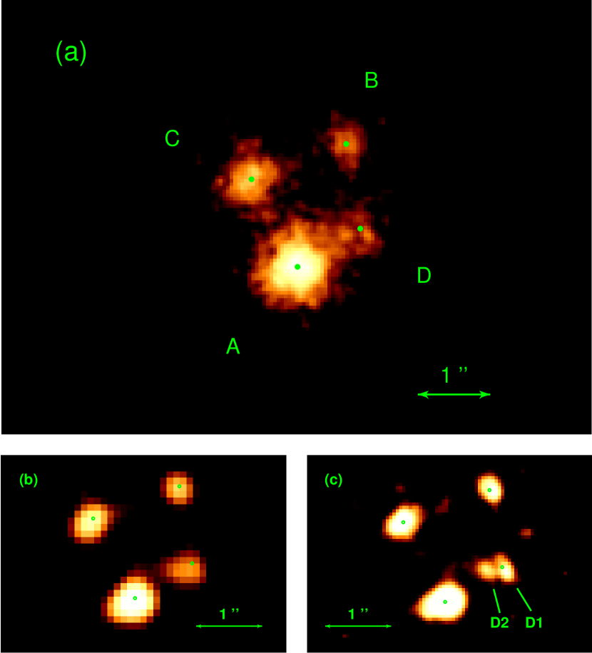
Figure 1: (a) The raw image of the combined observations of QSO 2237+0305  binned with a binsize of 0${}^{\prime\prime}\!\!.$05 and smoothed with a Gaussian of 0${}^{\prime\prime}\!\!.$05 (top). (b) The deconvolved image binned with a binsize of 0${}^{\prime\prime}\!\!.$1 (bottom left). (c) The deconvolved image binned with a binsize of 0${}^{\prime\prime}\!\!.$05 (bottom right). The green circles in each image are the corresponding HST image positions provided by CASTLES (http://cfa-www.harvard.edu/glensdata/Individual/Q2237.html).

The image of QSO 2237+0305 obtained by combining the two Chandra observations is shown in Figure 1a. The image is binned with a binsize of 0${}^{\prime\prime}\!\!.$05 and smoothed with a Gaussian with $\sigma$ = 0${}^{\prime\prime}\!\!.$05. Images B and C of QSO 2237+0305 are clearly resolved in Figure 1a. Images A and D are not well resolved, but since image A is the brightest image, it is less contaminated by image D. Moreover, the raw binned image of D seems to have two concentrations of photons separated by about 0${}^{\prime\prime}\!\!.$3.

The Lucy-Richardson deconvolution technique (Richardson, 1972; Lucy, 1974) was applied to the combined image in order to resolve the four images. We binned the X-ray events with binsizes of 0${}^{\prime\prime}\!\!.$1 and 0${}^{\prime\prime}\!\!.$05 for the deconvolution. The deconvolved images are shown in Figures 1b and 1c. In Figure 1b (image binsizes of 0${}^{\prime\prime}\!\!.$1), a total of four images are resolved, which is consistent with previous observations in other wave bands, while in Figure 1c (image binsizes of 0${}^{\prime\prime}\!\!.$05), five images in total are resolved.

The relative X-ray positions of the different images with respect to image A are obtained from the centroids of the deconvolved images. X-ray image positions are listed in Table 2 together with the HST positions obtained by CASTLES. The relative positions of images B and C with respect to A as measured with the deconvolution using a 0${}^{\prime\prime}\!\!.$1 binsize are consistent with the HST positions to 0${}^{\prime\prime}\!\!.$03. The separations between image D and the remaining images, A, B, and C as measured with the deconvolution using a 0${}^{\prime\prime}\!\!.$1 binsize differ from those measured in the optical by 0${}^{\prime\prime}\!\!.$09, 0${}^{\prime\prime}\!\!.$06, and 0${}^{\prime\prime}\!\!.$07, respectively. The expected observational uncertainties of the image positions are $\sigma=\alpha/\sqrt{S/N}$, where $\alpha$ is the spatial resolution of ACIS and S/N is the signal-to-noise ratio of the image. By accounting for the contamination of image D by image A , we estimate the uncertainty in the position of image D to be about 0${}^{\prime\prime}\!\!.$1. Thus, the discrepancy between the optical and X-ray positions of image D relative to image A is about $1\sigma$.

4 Spectral Analysis

Spectral analysis was carried out with the software tool XSPEC V11.2 (Arnaud, 1996). The total spectrum of all images of QSO 2237+0305 was extracted from a circle of 3^′′ radius centered on the centroid of the images. The spectra of images A, B, and C were extracted from circles of 1^′′ radii centered on the images, and the spectrum of image D was extracted from a circle of 0.6^′′ radius centered between D1 and D2 in order to avoid the contamination from the brightest image A. The background was extracted from an annulus centered on the centroid of the images with inner and outer radii of 5^′′ and 30^′′, respectively. All spectra were fitted in the 0.4–8 keV energy range assuming Galactic absorption of $\hbox{${N}_{\rm H}$}=5.5\times 10^{20}\hbox{cm${}^{-2}$}$ (Dickey & Lockman, 1990). We have applied a correction to the ancillary response files to account for the use of relatively small extraction regions. We determined the corrections to the ancillary response files by simulating the spectra of point sources at the locations of the images with and without apertures used in our analysis. For our simulations we used XSPEC to generate the source spectra and the raytrace tool MARX to model the dependence of photon scattering with energy. To account for the recently observed quantum efficiency decay of ACIS, possibly caused by molecular contamination of the ACIS filters, we have applied a time-dependent correction to the ACIS quantum efficiency implemented in the XSPEC model ACISABS1.1. ACISABS is an XSPEC model contributed to the Chandra users software exchange web-site http://asc.harvard.edu/cgi-gen/cont-soft/sof t-list.cgi. The ACIS quantum efficiency decay is insignificant for energies above 1 keV and does not affect the main results of our analysis.

4.1 Simple Absorbed Power-law Models

We began by fitting the spectra of the individual images and the spectrum of all images of QSO 2237+0305  from each epoch with a simple power law modified by Galactic absorption and neutral absorption placed at the redshift of the lens ($z=0.0395$). To obtain tighter constraints on the model parameters we fitted the spectra from both epochs simultaneously. In the case of the simultaneous fits, the model parameters, $\Gamma$ and ${N}_{\rm H}$ were kept the same between observations, whereas, the normalization parameters were allowed to vary independently. We also followed a different approach of fitting the combined spectra from both epochs. In the case of the combined spectra we weighted the ancillary response files from each observation. The spectral fitting results are listed in Table 3. The simultaneous fits (fits 7-11 of Table 3) and the combined fits (fits 12-16 of Table 3) to the spectra of QSO 2237+0305  yield consistent results. We will use the results from the combined spectra of both epochs in the remaining analysis since they provide slightly tighter constraints. The fit to the spectrum of all images for the combined observations yields a photon index of $\Gamma=1.90^{+0.05}_{-0.05}$ and a column density of $\hbox{${N}_{\rm H}$}=0.02^{+0.01}_{-0.01}\times 10^{22}\hbox{cm${}^{-2}$}$. The column density is relatively low compared to that detected in other galaxies. In Figure 2 we show the 68% confidence contours of ${N}_{\rm H}$ versus photon indices for all images. Absorption from gas in the lensing galaxy is marginally detected (at the 68% confidence level) towards image C. For the lines of sight towards the remaining images we can only place upper limits on the neutral hydrogen column densities from the lensing galaxy. In Table 3 we also list the 0.4–8 keV X-ray fluxes for fits 1—6. The fluxes of individual images were normalized based on the PSF fitting results in section 3. The total 0.4–8 keV fluxes for the first and second observations of QSO 2237+0305 are $4.6^{+0.4}_{-0.2}\times 10^{-13}\hbox{erg~{}cm${}^{-2}$~{}s${}^{-1}$}$, and $3.7^{+0.6}_{-0.5}\times 10^{-13}\hbox{erg~{}cm${}^{-2}$~{}s${}^{-1}$}$, and 0.4–8.0 keV lensed luminosities are $1.0\times 10^{46}\hbox{erg~{}s${}^{-1}$}$, and $8.3\times 10^{45}\hbox{erg~{}s${}^{-1}$}$, respectively. These luminosities have to be corrected by the lensing magnification in order to obtain the true luminosity of the quasar. The range of macro magnification was estimated from a few up to many hundred (Wambsganss & Paczy$\acute{\rm{n}}$ski, 1994), and a recent model from Schmidt, Webster, & Lewis (1998) estimated the magnification to be $16^{+5}_{-4}$.

4.2 Features in the Spectrum of Image A

Figure 3a shows the spectrum of image A combined from both observations of QSO 2237+0305 overplotted with a simple absorbed power law model described in $\S$4.1. The spectrum shows residuals in the 2–3 keV band, and the residuals are near the red-shifted energy of the Fe K$\alpha$ line. For a comparison in Figure 3b we show the combined spectrum of images B, C, and D for both observations overplotted with the best fit spectral model. In the combined spectrum of B, C, and D we detect residuals in the 2–3 keV band. However, these residuals are not as significant as those in image A and the peaks of the residuals differ between the two spectra. To model the residuals in image A we added a redshifted Gaussian line component to the absorbed power-law model and present the best fit parameters in Table 4. The line energy and width are kept free parameters during the fitting. Including a Gaussian emission line in our model for the spectrum of image A leads to a significant improvement in fit quality at the 99.99% confidence level (according to the $F$-test). The best-fit rest-frame energy, width, and equivalent width of the modeled emission line in the spectrum of image A are $E_{line}$ = $5.7_{-0.3}^{+0.2}$ keV, $\sigma_{line}$ = $0.87_{-0.15}^{+0.30}$ keV, and $EW=1200^{+300}_{-200}$ eV, respectively. We also modeled the combined spectrum of images B, C, and D with a redshifted Gaussian component. The improvement of the fit is significant at the 94% level based on the $F$-test. The rest-frame energy of the modeled Gaussian line of the combined spectrum of images B, C, and D is $E_{line}$ = $6.6_{-0.2}^{+0.1}$ keV and its width is consistent with that of a narrow line.

Protassov et al. (2002) argued that the F-test cannot be applied to assess the significance of a line component in a spectral model because when the null values of the additional parameters (in our case these are the parameters of the Gaussian line) fall on the boundary of the allowable parameter space, the reference distribution does not follow a F-distribution in general. Protassov et al. (2002) proposed the method of posterior predictive p-value, a Monte-Carlo simulation approach, to calibrate the sample distribution of the F-statistic. We followed this approach to calibrate the sample distribution of the F-statistic for the case of the spectrum of image A combined from both observations of QSO 2237+0305. The parameters of the null model (powerlaw with Galactic absorption and absorption at the lens) are well constrained from the spectrum of $\sim 1800$ photons and the simple approach described in section 5.2 of Protassov et al. (2002) is used. We simulated 10,000 spectra with XSPEC from the null model with parameters fixed at their best fit value. Each simulated spectrum, was binned as the real data and fitted with the null model and the alternative model (which included an additional line component). The F-statistic between null and the alternative model was calculated for each simulation. The results of the Monte-Carlo simulation are displayed in Figure 4. The maximum value of the F-statistics from the 10,000 simulated spectra is 7.28. Therefore, the F-statistic value of 7.74 obtained from the real spectrum of image A indicates that the null model (which does not include an emission line) is rejected at the $>$ 99.99% confidence level. In addition, we also compared the Monte-Carlo simulated sample distribution with the analytical F-distribution in Figure 4. The two distributions are consistent in this particular case.

5 Discussion

Our spatial analysis of the Chandra observations of QSO 2237+0305 has resolved the four lensed images A, B, C, and D, with positions in good agreement with those obtained from HST observations of QSO 2237+0305, however, both the raw and deconvolved Chandra data of QSO 2237+0305 hint to the presence of a fifth image near image D. In section 5.1 we investigate plausible mechanisms that can explain the fifth image. The analysis of the individual spectra of the images of QSO 2237+0305 indicates the presence of absorption from the lensing galaxy. In section 5.2 we compare the column densities obtained from our X-ray analysis with the column densities inferred from the $g-i$ color changes of the images. This comparison is used to estimate the dust-to-gas ratio in the lensing galaxy. In section 5.3 we compare the optical and X-ray image flux ratios. An exciting finding of our spectral analysis was the identification of a broad emission line near the energy of the redshifted Fe K$\alpha$ line in only image A. In section 4.2 we performed Monte Carlo simulations to show that the line in image A is significant at the 99.99% level. In section 5.4 we rule out possible instrumental effects that could mimic such a line and discuss possible origins of the broad Fe K$\alpha$ line. We discuss the variability of the source in section 5.5

5.1 An Additional Image?

The Chandra observations of QSO 2237+0305 indicate an additional image when the data is binned with a binsize of less than 0${}^{\prime\prime}\!\!.$07 both in the raw image and in the deconvolved image. The total number of photons detected in both images D1 and D2 combining the two observations of QSO 2237+0305 is $\sim 340$, thus the apparent image splitting could be the result of poor photon statistics. The difference between the optical and X-ray positions of image D is larger than that measured in the other images. This large difference in image D may be the result of the significant contamination of this image by the brighter image A. Considering the 0${}^{\prime\prime}\!\!.$3 separation of D1 and D2, their X-ray fluxes, and the fact that the additional images only show up in the X-ray band, it would be extremely difficult to interpret this result, if the images D1 and D2 are real. Here we briefly investigate possible origins (other than the mentioned statistical interpretation) for the discrepancy between the optical and X-ray image configuration of QSO 2237+0305.

(a) Spatially distinct X-ray flares in the source plane.
X-rays are generated in the inner most region of the accretion disc. X-ray variability studies of quasars indicate that the size of the X-ray continuum emission region is of the order of $\sim$ 1 $\times$ 10^-4 pc (e.g., Chartas et al. 2001). If we were to attribute the additional X-ray image to macrolensing or microlensing of two distinct X-ray flares the implied distance between flares would be about 2 kpc in the source plane, considerably larger than the expected size of the X-ray emitting region. The flares would also have to vary over time-scales shorter than the time-delay between the images since only one additional image is observed if we attribute it to macrolensing.

(b) An additional X-ray source in the lens plane.
The luminosity of the additional image would be $\sim 10^{41}\hbox{erg~{}s${}^{-1}$}$ if the source producing the image were located in the lensing galaxy, and this is over two orders of magnitude brighter than the Eddington limit for X-ray binaries. This luminosity, however, lies at the upper end of the luminosity range ($10^{39-41}\hbox{erg~{}s${}^{-1}$}$, e.g., Roberts et al. 2002) of ultraluminous X-ray (ULX) sources.

(c) An X-ray jet component extending from image A.
This is unlikely based on VLA observations that indicate (Falco et al., 1996) QSO 2237+0305 being a radio quiet quasar with no jet.

(d) A source in our Galaxy.
The X-ray luminosity of the additional image would be $\sim 10^{36}\hbox{erg~{}s${}^{-1}$}$ if it were located in the Galaxy, and any object with such a large X-ray luminosity would have been detected by HST.

(e) A fifth image produced by the lensing galaxy.
In principle, a gravitational macrolens could generate an odd number of images if the lens potential is non-singular. But the anticipated position of the central image should lie within the central core of the lens potential and be greatly demagnified, which is not consistent with the Chandra observations of QSO 2237+0305.

(f) Microlensing by solar-mass stars in the central bulge of the lensing galaxy.
The image separation produced by a microlens of mass M is given by the expression $\alpha_{0}\approx 3\times 10^{-3}\sqrt{M/\hbox{${M}_{\odot}$}}(D_{OL}/kpc)^{1/2}$ arcsec (Schneider et al., 1992), where $D_{OL}$ is the angular diameter distance between observer and lens. The interpretation of the 0${}^{\prime\prime}\!\!.$3 image splitting of image D as a microlensing event would require a microlens mass of at least $\sim 10^{8}\hbox{${M}_{\odot}$}$. The Einstein radius of the microlens at the source plane is proportional to the square-root of the mass of the microlens, specifically for this system, $R_{E}=1.1\times 10^{17}~{}M^{1/2}h^{-1/2}$ cm. The optical and radio images should also show this splitting if such a large “microlens” were present, unless the optical and radio emission regions are far more extended than the Einstein radius. This could possibly be true for the radio emission, but studies of microlensing of QSO 2237+0305 showed that the optical emission region is within 1 pc of the accretion disc of the central engine (Yonehara, 2001), which make the above interpretation highly improbable.

5.2 Absorption at the Lensing Galaxy

In the appendix of Agol, Jones, & Blaes (2000), the extinctions for the images of QSO 2237+0305 were estimated based on the $g-i$ color changes between the images (Yee, 1988), and the correlation between the $g-i$ color change and the lens galaxy surface brightness (Racine, 1991). The hydrogen column densities can be inferred from the extinction by assuming an extinction law of $R=3.1\pm 0.9$ from the Milky Way and employing a dust-to-gas ratio of ${N}_{\rm H}$= $5.9\times 10^{21}~{}E_{B-V}~{}mag^{-1}~{}cm^{-2}$ (Bohlin, Savage, & Drake, 1978). A comparison between ${N}_{\rm H}$ obtained from our spectral fits to the Chandra data of QSO 2237+0305 and the inferred values from the extinctions is presented in Table 5. The comparison shows that the column densities inferred from the extinction values are systematically larger than the column densities obtained from our X-ray analysis by about $2.1\sigma$, $2.5\sigma$, $2.6\sigma$, and $2.7\sigma$ for images C, B, A, and D, respectively. The ratio of the column densities obtained from our X-ray analysis to those inferred from the extinction values are about 20%, 13%, 6%, and 5% for image C, B, A, and D, respectively. The estimated large value for ${N}_{\rm H}$ inferred from the extinction measurements could arise from a problem with one of our two assumptions; the extinction law and the gas-to-dust ratio taken to be that of the Milky Way. The extinction law of the lensing galaxy 2237+0305 has been measured by Nadeau et al. (1991) assuming $A(K)/A(V)=0.11$, where A(K) and A(V) are the extinctions in the K band and V band, respectively. They find that the resulting extinction law in QSO 2237+0305 is in good agreement with that of the Milky Way. Thus, we are left with the possibility that the dust-to-gas ratio of the lensing galaxy 2237+0305 is significantly larger than that of the Milky Way. The dust-to-gas ratios for several gravitational lenses are discussed by Falco et al. (1999). They found that the dust-to-gas ratios are small for the systems B0218+357 and PKS 1830-211, which is opposite to what we observed in QSO 2237+0305.

5.3 Image Flux Ratios

It is well established from optical monitoring that QSO 2237+0305 is being microlensed as mentioned in the introduction section. We compared the X-ray flux ratios of QSO 2237+0305 with the optical V band flux ratios from the Optical Gravitational Lensing Experiment (OGLE) monitoring data obtained only four days prior to our first observation. An optical flux close to our second observation was not available. The OGLE website is at http://bulge.princeton.edu/~ogle. The extinction for the optical data is corrected based on the method described in appendix of Agol, Jones, & Blaes (2000). To compute the X-ray flux ratios we used the 2–8 keV band to avoid the complication of absorption which may affect the soft energy band to a greater degree. The results from this comparison are presented in Table 6. The X-ray and optical V band flux ratios of images B, C, and D relative to image A are consistent. Since the optical fluxes are influenced by microlensing the agreement between X-ray and optical V band flux ratios implies that the X-ray fluxes are also magnified by microlensing. We also listed the 2–8 keV flux ratios, with larger error bars though, for the second observation in Table 6.

5.4 Broad Fe K$\alpha$ Line

Our spectral analysis indicates the presence of significant residuals between energies of 2–3 keV in image A. This energy region is near the energy of the red-shifted Fe K$\alpha$ line. Unfortunately, these residuals fall near a sudden change of the HRMA/ACIS effective area caused by the iridium M absorption edges of the Chandra mirrors. To ascertain any systematic calibration uncertainties near the mirror edge we have fit the spectra of several test-sources with expected smooth power-law spectra near the 2 keV iridium edge. Since $\chi^{2}$ residuals depend on the statistics, we filtered the test-source data in time to produce spectra with a total number of counts equal to that observed in the second observation of QSO 2237+0305. Typical residuals for these test-sources near the mirror edge are less than $\sim$ 1$\sigma$ indicating that the observed consecutive 2$\sigma$ residuals near 2 keV in the spectrum of image A are real and not due to systematic errors in the calibration of the effective area of the Chandra mirrors. We also note that the residuals are more significant in image A (at the 99.99% confidence level) than the combined spectrum of images B, C, and D (at the 94% confidence level). Furthermore, the energies and widths of the lines in image A and the remaining images differ significantly. It is unlikely that the residuals are caused by pile-up. We simulated, using the software tool LYNX (see appendix A of Chartas et al. 2000), a piled-up spectrum with input model parameters taken from fit 2 of Table 3 and using the observed count rate in image A of 0.16 counts per frame. We find no evidence that the residuals are due to pile up. To further test whether pile up is the cause of the observed residuals, we excluded events from the core of image A. After the removal of the core, the remaining spectrum of image A still shows residuals between 2 and 3 keV. We conclude that a broad Fe K$\alpha$ line is present in the spectrum of image A.

The presence of a broad Fe K$\alpha$ line in image A and not in the other images is indicative that microlensing may be enhancing the redshifted emission near the black hole. Observational and theoretical arguments rule out interpretations other than microlensing. First, strong and broad Fe K$\alpha$ lines detected in several low luminosity Seyfert galaxies are rarely observed in quasars. This fact is further supported by the observed anti-correlation between the luminosities of AGN and the equivalent widths of Fe K$\alpha$ lines detected in these AGN (Iwasawa & Taniguchi, 1993; Nandra et al., 1995) and by theoretical estimates of the properties of Fe K$\alpha$ lines in quasars (Fabian et al., 2000). Recently, Fe K$\alpha$ lines with equivalent widths of $\sim$ 1 keV were observed in the quasars H 1413+117  (Oshima et al., 2001; Chartas et al., 2003) and MG J0414+0534 (Chartas et al., 2002). However, these quasars are both gravitationally lensed and these relatively large equivalent widths were interpreted as the result of microlensing (Chartas et al., 2002; Popovi$\acute{\rm{c}}$ et al., 2002; Chartas et al., 2003). Second, an interpretation suggesting that the broad line in image A of QSO 2237+0305 is being emitted by an X-ray flare which is only seen in image A is not supported by the Chandra observations. In particular, the predicted time-delays between images A and B, A and C, and A and D are $\sim$ 2, 16, and 5 hours, respectively (Schmidt, Webster, & Lewis, 1998). If the flare duration is longer than a few days, we would have detected a similar enhanced and broadened Fe K$\alpha$ line in the spectrum of the combined images of B, C, and D, since the relative time-delays are less than a day. For a flare duration of less than $\sim~{}8.4$ hours we would have detected significant variability of the strength and shape of the Fe K$\alpha$ line during the first observation. We did not detect such variability during the first observation, and therefore, rule out flares with durations of less than 8.4 hours as being responsible for the broad Fe K$\alpha$ line detected in image A only.

In the following arguments we assume that the difference between the spectrum of image A and the combined spectrum of images B, C, and D is produced by microlensing, which magnifies the inner part of the accretion disc. The broadening and the observed redshift of the Fe K$\alpha$ line in the spectrum of image A imply that the emission originates near the center of the black hole where special and general relativistic effects are important. The broad and redshifted profile of the Fe K$\alpha$ line and its large equivalent width also indicate that the microlensing caustic should be located near the broad Fe K$\alpha$ line emission region. The broad Fe K$\alpha$ line emission region where special and general relativistic effects are important is expected to be very small $\sim 10~{}r_{g}$ and the magnification of this relatively small emission region close to a fold caustic scales approximately as the inverse square root of its distance to the caustic. This microlensing event is fundamentally different from those discussed in theoretical studies of optical and UV broad emission lines (e.g. Popovi$\acute{\rm{c}}$, Mediavilla, & Mu$\tilde{\rm{n}}$oz 2001; Abajas et al. 2002) in that the locations and sizes of the emission regions and the line broadening mechanisms are all different. Popovi$\acute{\rm{c}}$ et al. (2002) discussed the influence of microlensing on the shape of the Fe K$\alpha$ line in AGN. A qualitative comparison between the profile of the observed broad Fe K$\alpha$ line in image A and the theoretical predictions of Popovi$\acute{\rm{c}}$ et al. (2002) also indicates that the microlensing caustic should be located near the broad Fe K$\alpha$ line emission region.

The microlensing interpretation has to explain the following facts indicated by the comparison of the optical and X-ray observations of QSO 2237+0305. First, the OGLE photometric data show no peak in the V band light-curve of image A during the September 2000 observation. The V band light-curve of image A shows a microlensing event that peaked about ten months earlier than the first Chandra observation. Delays between the peaks of the X-ray and optical light-curves have been simulated to occur in caustic crossings in the case where the X-ray and optical emission regions differ significantly (Mineshige, Yonehara, & Takahashi, 2001). As we mentioned earlier the estimated size of the X-ray broad Fe K$\alpha$ line region where special and general relativistic effects would produce the observed distortion of the Fe K$\alpha$ line is $\sim$ 10 $r_{g}$, whereas, the size of the optical and X-ray continuum emission regions are $\lower 2.0pt\hbox{$\,\buildrel\scriptstyle<\over{\scriptstyle\sim}\,$}6\times 10^{15}$ cm and $\sim 1\times 10^{14}$ cm, respectively. The size of the X-ray continuum region is based on the observed X-ray variability of the continuum in image A of about $\sim$ 3000 sec (proper time) which corresponds to a size of about $\sim 1\times 10^{14}$ cm (see section 5.5 for more details). The optical emission region has been constrained to be $\,\buildrel\scriptstyle<\over{\scriptstyle\sim}\,$ 6 $\times$ 10¹⁵ cm (Wyithe et al., 2000). These sizes of emission regions are similar to those assumed in the simulations performed by Mineshige, Yonehara, & Takahashi (2001) that showed significant delays in the peaks of the magnification light-curves originating from different emission regions. We note that the radiation mechanisms assumed for the emission regions in the simulations of Mineshige, Yonehara, & Takahashi (2001) may differ from those in QSO 2237+0305, however, the main contribution to the simulated delays in the peaks arises from the different sizes of the emission regions. Second, the optical and X-ray continuum flux ratios are consistent within $1\sigma$ at the time of the first Chandra observation. This is possible since both the X-ray and optical continuum regions are much larger than the Fe K$\alpha$ line emission region, as we discussed above, and they are both comparable in size with the Einstein radius of a typical 0.1 ${M}_{\odot}$ microlens. The simulations of Mineshige, Yonehara, & Takahashi (2001) also showed that the flux magnifications for the X-ray and optical extended emission regions are not significantly different during the microlensing event. Detailed modeling of a caustic crossing that includes both the optical and X-ray constraints of QSO 2237+0305 are needed to accurately interpret the microlensing event in QSO 2237+0305. However, such an analysis is beyond the scope of this paper.

5.5 Variability

We investigated the long term variability of QSO 2237+0305 by comparing the fluxes of the two Chandra observations with the flux observed in the previous ROSAT observation. The 0.4–8 keV and 0.1–2.4 keV fluxes of QSO 2237+0305 are $4.6\times 10^{-13}\hbox{erg~{}cm${}^{-2}$~{}s${}^{-1}$}$ and $2.3\times 10^{-13}\hbox{erg~{}cm${}^{-2}$~{}s${}^{-1}$}$, respectively, for the first Chandra observation. The 0.1–2.4 keV flux detected with the first Chandra observation is consistent with that previously detected with ROSAT (Wambsganss et al., 1999). A comparison between the two Chandra observations of QSO 2237+0305 shows that the total 0.4–8 keV flux has decreased by about 20% in the second observation. It is not clear from the present Chandra data if this decrease in X-ray flux is caused by intrinsic variability of the quasar or by microlensing.

We also explored the variability of QSO 2237+0305 within each observation. The light-curves of the combined images and the individual images A, B, C, and D for the first and second observation are displayed in Figure 5. We performed Kolmogorov-Smirnov (K-S) tests to the unbinned light-curves of each image. The K-S test results are listed in Table 7. The K-S results indicate that the light-curve of image A for the first observation is variable at the 97% confidence level. The K-S plot of the cumulative probability distribution versus the exposure number for image A of the first observation is illustrated in Figure 6. The light-curve of the combined images for the first observation also shows some variability according to the K-S test, however, at a lower $\sim$ 90% confidence level. In this light-curve we identified two possible flux enhancements. A comparison between the light-curve of all images and that of image A indicated that the first enhancement in the total light-curve corresponds to the bump detected at a similar time in the light-curve of image A. The correspondence of the second flux enhancement of the total light-curve with bumps in individual light-curves is less clear than the first bump. It is possible that the second bump arises in image B. We performed an auto-correlation of the total light-curve for the first observation and obtained a lag of 5 bins (1 bin = 1944.6 seconds) which yields a maximum auto-correlation coefficient of 0.40. The probability of obtaining this auto-correlation coefficient by chance is 0.06. We tested the sensitivity of the computed lag-time to the selected bin size of the total light-curve by performing the auto-correlation over a range of bin sizes. In all cases we recovered lag-times similar to the one obtained above. Our simple auto-correlation analysis indicated a possible time-delay of $2.7^{+0.5}_{-0.9}~{}hours$ in the total light-curve of QSO 2237+0305 for the first Chandra observation. The errors of this time-delay are dominated by the different choices of the bin size. A comparison between the total light-curve and those of the individual images indicates that the measured time-delay most likely corresponds to the time-delay between images A and B with image A leading. This is consistent with recent modeling of (Schmidt, Webster, & Lewis, 1998) that predict a time-delay between images A and B of $2.0^{+0.4}_{-0.3}~{}h_{75}^{-1}$ hours with image A leading.

6 Conclusions

1. Chandra observations of QSO 2237+0305 have resolved the system into at least four X-ray images. A possible fifth image could be the result of poor photon statistics and the contamination from the brightest image A. A longer Chandra observation of QSO 2237+0305 is needed to resolve this issue.

2. The X-ray flux ratios of images B, C, and D with respect to image A are consistent with the V band flux ratios observed only four days prior to our first Chandra observation. This indicates that the X-ray fluxes are also magnified by microlensing as expected since the X-rays are thought to originate from the inner most regions of the accretion disc.

3. The hydrogen column densities of images A, B, C, and D measured from the Chandra observations of QSO 2237+0305 are significantly lower than the column densities inferred from extinction measurements of these images in the optical and infrared bands. This difference is suggestive of a higher value of the dust-to-gas ratio in the lensing galaxy compared to the Galactic value.

4. Our spectral analysis indicates the presence of a broad Fe K$\alpha$ line in image A with a rest-frame energy, width, and equivalent width of $E_{line}$ = $5.7_{-0.3}^{+0.2}$ keV, $\sigma_{line}$ = $0.87_{-0.15}^{+0.30}$ keV and $EW=1200^{+300}_{-200}$ eV, respectively. The enhancement of the emission line in image A is possibly caused by microlensing since the combined spectrum of the other three images does not show such a significant feature. The redshift and broadening of the line may be the result of the Doppler effect and special and general relativistic effects.

5. QSO 2237+0305 exhibits variability both over long and short time scales from the Chandra observations. The X-ray flux has dropped by 20% between the two observations, and the Kolmogorov-Smirnov test showed that image A is variable at the 97% confidence level within the first observation. A possible time-delay of $2.7^{+0.5}_{-0.9}~{}hours$ between images A and B with image A leading is detected in the first Chandra observation.

Table 1: Chandra Observations of QSO 2237+0305

Observation	Exposure	Total	$\rm{R_{Total}}$	$\rm{R_{A}}$	$\rm{R_{B}}$	$\rm{R_{C}}$	$\rm{R_{D}}$	$\rm{R_{Bkg}}$
Date	$\rm{s}$	Counts	$\rm{10^{-3}~{}cnts~{}s^{-1}}$					$\rm{10^{-6}~{}cnts~{}(^{\prime\prime})^{-2}~{}s^{-1}}$
2000-09-06	30287	2635	$86.9\pm 1.7$	$47.3\pm 1.3$	$10.0\pm 0.6$	$19.0\pm 0.8$	$10.6\pm 0.7$	$4.5\pm 0.2$
2001-12-08	9538	608	$63.6\pm 2.6$	$36.1\pm 2.0$	$7.3\pm 0.9$	$12.1\pm 1.2$	$8.1\pm 1.0$	$4.0\pm 0.4$

Table 2: Relative Optical and X-ray Positions of QSO 2237+0305 Images

Telescope	Offset	A	B	C	D	D1	D2
		arcsec	arcsec	arcsec	arcsec	arcsec	arcsec
HST	RA	0	$-0.673\pm 0.003$	$0.635\pm 0.003$	$-0.866\pm 0.003$	…	…
	DEC	0	$1.697\pm 0.003$	$1.210\pm 0.003$	$0.528\pm 0.003$	…	…
Chandra	RA	0	$-0.67\pm 0.02$	$0.63\pm 0.02$	$-0.78\pm 0.03$	…	…
	DEC	0	$1.73\pm 0.02$	$1.21\pm 0.02$	$0.49\pm 0.03$	…	…
Chandra	RA	0	$-0.68\pm 0.02$	$0.62\pm 0.02$	…	$-0.93\pm 0.04$	$-0.67\pm 0.04$
	DEC	0	$1.72\pm 0.02$	$1.21\pm 0.02$	…	$0.46\pm 0.04$	$0.46\pm 0.04$

Table 3: Results of Fits to the Chandra Spectra of QSO 2237+0305

Fit	Epoch	Image	$\Gamma$	$\rm{N_{H}}(z=0.0395)$	Flux	$\chi^{2}_{\nu}(\nu)$	$P(\chi^{2}/{\nu})$
				$10^{22}~{}\rm{cm^{-2}}$	$10^{-13}~{}\rm{erg~{}s^{-1}~{}cm^{-2}}$
1	I	Total	$1.90^{+0.06}_{-0.05}$	$0.02^{+0.01}_{-0.02}$	$4.6^{+0.4}_{-0.2}$	1.22(124)	0.05
2	I	A	$1.81^{+0.07}_{-0.07}$	$0.01^{+0.02}_{-0.01}$	$2.5^{+0.2}_{-0.2}$	1.25(76)	0.07
3	I	B	$1.70^{+0.15}_{-0.12}$	$0.00^{+0.03}_{-0.00}$	$0.5^{+0.1}_{-0.1}$	1.11(15)	0.34
4	I	C	$1.93^{+0.07}_{-0.08}$	$0.05^{+0.03}_{-0.04}$	$1.0^{+0.1}_{-0.1}$	0.87(35)	0.68
5	I	D	$1.78^{+0.18}_{-0.12}$	$0.00^{+0.03}_{-0.00}$	$0.7^{+0.1}_{-0.1}$	0.75(12)	0.70
6	II	Total	$1.88^{+0.12}_{-0.12}$	$0.03^{+0.03}_{-0.03}$	$3.7^{+0.6}_{-0.5}$	1.26(33)	0.14
7	I+II simultaneous	Total	$1.90^{+0.06}_{-0.06}$	$0.02^{+0.01}_{-0.02}$	…	1.22(159)	0.03
8	I+II simultaneous	A	$1.81^{+0.07}_{-0.07}$	$0.01^{+0.02}_{-0.01}$	…	1.31(96)	0.02
9	I+II simultaneous	B	$1.69^{+0.14}_{-0.11}$	$0.00^{+0.02}_{-0.00}$	…	1.10(18)	0.34
10	I+II simultaneous	C	$1.90^{+0.14}_{-0.14}$	$0.04^{+0.04}_{-0.03}$	…	0.83(41)	0.78
11	I+II simultaneous	D	$1.83^{+0.16}_{-0.13}$	$0.00^{+0.03}_{-0.00}$	…	0.70(15)	0.78
12	I+II combined	Total	$1.90^{+0.05}_{-0.05}$	$0.02^{+0.01}_{-0.01}$	…	1.02(149)	0.40
13	I+II combined	A	$1.79^{+0.06}_{-0.07}$	$0.01^{+0.01}_{-0.01}$	…	1.06(94)	0.32
14	I+II combined	B	$1.73^{+0.12}_{-0.10}$	$0.00^{+0.02}_{-0.00}$	…	1.26(20)	0.20
15	I+II combined	C	$1.91^{+0.08}_{-0.07}$	$0.05^{+0.03}_{-0.03}$	…	0.89(41)	0.68
16	I+II combined	D	$1.86^{+0.14}_{-0.13}$	$0.00^{+0.02}_{-0.00}$	…	1.13(16)	0.32

Table 4: Fits to the Spectrum of Image A and the Combined Spectrum of Images B, C, and D of QSO 2237+0305 with and without an Fe line Model

Fit	Epoch	Image	Model	$\Gamma$	$\rm{N_{H}}(z=0.0395)$	$\rm{E_{line}}$	$\sigma$	EW	$\chi^{2}_{\nu}(\nu)$	$P(\chi^{2}/{\nu})$
					$10^{22}~{}\rm{cm^{-2}}$	$\rm{keV}$	$\rm{keV}$	$\rm{eV}$
1	I+II	A	pow	$1.80^{+0.06}_{-0.07}$	$0.01^{+0.01}_{-0.01}$	…	…	…	1.04(73)	0.38
2	I+II	A	pow+Gaussian	$1.83^{+0.07}_{-0.06}$	$0.00^{+0.02}_{-0.00}$	$5.7^{+0.2}_{-0.3}$	$0.87^{+0.30}_{-0.15}$	$1200^{+300}_{-200}$	0.82(70)	0.87
3	I+II	B+C+D	pow	$1.98^{+0.07}_{-0.13}$	$0.03^{+0.02}_{-0.02}$	…	…	…	0.87(58)	0.75
4	I+II	B+C+D	pow+Gaussian	$2.00^{+0.09}_{-0.08}$	$0.03^{+0.02}_{-0.02}$	$6.6^{+0.1}_{-0.2}$	$<0.30$	$400^{+300}_{-200}$	0.81(55)	0.85

Table 5: Hydrogen Column Densities in QSO 2237+0305 Images

	A	B	C	D
	$10^{21}~{}cm^{-2}$	$10^{21}~{}cm^{-2}$	$10^{21}~{}cm^{-2}$	$10^{21}~{}cm^{-2}$
Chandra	$0.1^{+0.1}_{-0.1}$	$0.0^{+0.2}_{-0.0}$	$0.5^{+0.3}_{-0.3}$	$0.0^{+0.2}_{-0.0}$
Converted Value	$1.7^{+0.6}_{-0.6}$	$1.6^{+0.6}_{-0.6}$	$2.5^{+0.9}_{-0.9}$	$2.2^{+0.8}_{-0.8}$

Table 6: X-ray and Optical Flux Ratio in QSO 2237+0305

Band	Date	A	B	C	D
V	2000 Sep 2	$1$	$0.24\pm 0.07$	$0.54\pm 0.19$	$0.29\pm 0.09$
X-Ray	2000 Sep 6	$1$	$0.23\pm 0.05$	$0.38\pm 0.06$	$0.27\pm 0.06$
X-Ray	2001 Dec 8	$1$	$0.27\pm 0.19$	$0.42\pm 0.22$	$0.19\pm 0.10$

Table 7: Kolmogorov-Smirnov Test of Variability for QSO 2237+0305

Epoch	Chance Probability
	Total	A	B	C	D
I	$0.11$	$0.03$	$0.80$	$0.95$	$0.08$
II	$0.97$	$0.70$	$0.15$	$0.86$	$0.49$

Figure 2: 68% confidence contours of photon index and neutral absorption at the lens ($z=0.0395$) for images A, B, C, and D of the combined spectra from both observations. The shaded region represents the overlapping region of the four confidence contours.

Figure 3: (a) Spectrum of image A combined from both observations (top). (b) Combined spectrum of images B, C, and D from both observations (bottom).

Figure 4: To evaluate the significance of the emission feature in image A, we determined the distribution of the F-statistic (shown as histogram) using a Monte-Carlo simulation. We also overplotted for comparison the analytical curve for the F-distribution (shown as dashed curve). The vertical line indicates the F value obtained from the real spectrum of image A. The simulation shows that the detection of the broad emission line is significant at the $>$ 99.99% confidence level.

Figure 5: The full band (0.2–10 keV) light-curves of the sum of all images and images A, B, C, and D, separately, for the first and second Chandra observations of QSO 2237+0305. The data were taken continuously within each observation.

Figure 6: Cumulative probability distribution vs. exposure number for image A of the first observation of QSO 2237+0305 compared to the cumulative probability distribution of a constant source.

References

- Abajas et al. (2002) Abajas, C., Mediavilla, E., Muoz, J. A., Popovi, L. ., & Oscoz, A. 2002, ApJ, 576, 640
- Agol, Jones, & Blaes (2000) Agol, E., Jones, B., & Blaes, O. 2000, ApJ, 545, 657
- Agol & Krolik (1999) Agol, E., & Krolik, J. 1999, ApJ, 524, 49
- Arnaud (1996) Arnaud, K. A. 1996, ASP Conf. Ser. 101: Astronomical Data Analysis Software and Systems V, ed. Jacoby G. & Barnes J., 17
- Bohlin, Savage, & Drake (1978) Bohlin, R. C., Savage, B. D., & Drake, J. F. 1978, ApJ, 224, 132
- Chartas et al. (2002) Chartas, G., Agol, E., Eracleous, M., Garmire, G. P., Bautz, M. W., & Morgan, N. D. 2002, ApJ, 568, 509
- Chartas et al. (2003) Chartas, G., Brandt, W. N., Gallagher, S. C., and Garmire G. P., 2003, Astronomische Nachrichten, in press
- Chartas et al. (2001) Chartas, G., Dai, X., Gallagher, S. C., Garmire, G. P., Bautz, M. W., Schechter, P. L., & Morgan, N. D. 2001, ApJ, 558, 119
- Chartas et al. (2000) Chartas, G., Worrall, D. M., Birkinshaw, M., Cresitello-Dittmar, M., Cui, W., Ghosh, K. K., Harris, D. E., Hooper, E. J., Jauncey, D. L., Kim, D.-W., Lovell, J., Mathur, S., Schwartz, D. A., Tingay, S. J., Virani, S. N., & Wilkes, B. J. 2000, ApJ, 542, 655
- Dickey & Lockman (1990) Dickey, J. M., & Lockman F. J. 1990, ARA&A 28, 215
- Fabian et al. (2000) Fabian, A. C., Iwasawa, K., Reynolds, C. S., & Young, A. J. 2000, PASP, 112, 1145
- Falco et al. (1999) Falco, E. E, Impey, C. D., Kochanek, C. S., Lehr, J., Mcleod, B. A., Rix, H. -W., Keeton, C. R., Muoz, J. A., & Peng, C. Y 1999, ApJ, 523, 617
- Falco et al. (1996) Falco, E. E., Lehr, J., Perley, R. A., Wambsganss, J., & Gorenstein, M. V. 1996, AJ, 112, 897
- Foltz et al. (1992) Foltz, C. B., Hewett, P. C., Webster, R. L., & Lewis, G. F. 1992, ApJ, 386, L43
- Garmire et al. (2002) Garmire, G. P., Bautz, M. W., Nousek, J. A., & Ricker, G. R. 2002, SPIE, 4851
- Huchra et al. (1985) Huchra, J., Gorenstein, M., Kent, S., Shapiro, I., Smith, G., Horine, E., & Perley, R. 1985, AJ, 90, 691
- Irwin et al. (1989) Irwin, M. J., Webster, R. L., Hewett, P. C., Corrigan, R. T., & Jedrzejewski, R. I. 1989, AJ, 98, 1989
- Iwasawa & Taniguchi (1993) Iwasawa, K., & Taniguchi, Y. 1993, ApJ, 413, L15
- Kayser & Refsdal (1989) Kayser, R., & Refsdal, S. 1989, Nature, 338, 745
- Kayser, Refsdal, & Stabell (1986) Kayser, R., Refsdal, S., & Stabell, R. 1986, A&A, 166, 36
- Kent & Falco (1988) Kent, S. M., & Falco, E. E. 1988, AJ, 96, 1570
- Lucy (1974) Lucy, L. B. 1974, AJ, 79, 745
- Mediavilla et al. (1998) Mediavilla, E., Arribas, S., del Burgo, C., Oscoz, A., Serra-Ricart, M., Alcalde, D., Falco., E. E., Goicoechea, L. J., García-Lorenzo, B., & Buitrago, J. 1998, ApJ, 503, L27
- Mineshige, Yonehara, & Takahashi (2001) Mineshige, S., Yonehara, A., & Takahashi, R. 2001, PASA, 18, 186
- Mori et al. (2001) Mori, K., Tsunemi, H., Miyata, E., Baluta, C., Burrows, D. N., Garmire, G. P., & Chartas, G. 2001, in ASP Conf. Ser. 251, New Century of X-Ray Astronomy, ed. H. Inoue & H. Kunieda (San Francisco: ASP), 576
- Nadeau et al. (1991) Nadeau, D., Yee, H. K. C., Forrest, W. J., Garnett, J. D., Ninkov, Z., & Pipher, J. L. 1991, ApJ, 376, 430
- Nandra et al. (1995) Nandra, K., Fabian, A. C., Brandt, W. N., Kunieda, H., Matsuoka, M., Mihara, T., Ogasaka, Y., & Terashima, Y. 1995, MNRAS, 276, 1
- Oshima et al. (2001) Oshima, T., Mitsuda, K., Fujimoto, R., Iyomoto, N., Futamoto, K., Hattori, M., Ota, N., Mori, K., Ikebe, Y., Miralles, J. M., & Kneib, J.-P. 2001, ApJ, 563, L103
- Østensen et al. (1996) Østensen, R., Refsdal, S., Stabell, R., Teuber, J., Emanuelsen, P. I., Festin, L., Florentin-Nielsen, R., Gahm, G., Gullbring, E., Grundahl, F., Hjorth, J., Jablonski, M., Jaunsen, A. O., Kass, A. A., Karttunen, H., Kotilainen, J., Laurikainen, E., Lindgren, H., Maehoenen, P., Nilsson, K., Olofsson, G., Olsen, Ø., Pettersen, B. R., Piirola, V., Sørensen, A. N., Takalo, L., Thomsen, B., Valtaoja, E., Vestergaard, M., & Av Vianborg, T. 1996, A&A, 309, 59
- Popovi et al. (2002) Popovi, L. ., Mediavilla, E. G., Jovanovi, P., & Muoz, J. A. 2002, astro-ph/0211523
- Popovi, Mediavilla, & Muoz (2001) Popovi, L. ., Mediavilla, E. G., & Muoz, J. A. 2001, A&A, 378, 295
- Protassov et al. (2002) Protassov, R., van Dyk, D. A., Connors, A., Kashyap, V. L., & Siemiginowska A. 2002, ApJ, 571, 545
- Racine (1991) Racine, R. 1991, AJ, 102, 454
- Racine (1992) Racine, R. 1992, ApJ, 395, L65
- Rauch et al. (2002) Rauch, M., Sargent, W. L. W., Barlow, T. A., & Simcoe, R. A. 2002, ApJ, 576, 45
- Richardson (1972) Richardson, W. H. 1972, J. Opt. Soc. Am., 62, 55
- Roberts et al. (2002) Roberts, T. P., Goad, M. R., Ward, M. J., Warwick, R. S., & Lira, P. 2002, astro-ph/0202017
- Schmidt, Webster, & Lewis (1998) Schmidt, R., Webster, R. L., & Lewis, G. F. 1998, MNRAS, 295, 488
- Schneider et al. (1988) Schneider, D. P., Turner, E. L., Gunn, J. E., Hewitt, J. N., Schmidt, M., & Lawrence, C. R. 1988, AJ, 95, 1619
- Schneider et al. (1992) Schneider, P., Ehlers, J., & Falco, E. E. 1992, Gravitational Lenses
- Tsunemi et al. (2001) Tsunemi, H., Mori, K., Miyata, E., Baluta, C., Burrows, D. N., Garmire, G. P., & Chartas, G. 2001, ApJ, 554, 496
- Wambsganss et al. (1999) Wambsganss, J., Brunner, H., Schindler, S., & Falco, E. 1999, A&A, 346, L5
- Wambsganss & Paczyski (1994) Wambsganss, J & Paczyski, B. 1994, AJ, 108, 1156
- Wyithe et al. (2000) Wyithe, J. S. B., Webster, R. L., Turner, E. L., & Mortlock, D. J. 2000, MNRAS, 315, 62
- Wise et al. (1997) Wise, M. W., Davis, J. E., Huenemoerder, Houck, J. C., Dewey, D., Flanagan, K. A., & Baluta, C. 1997, The MARX 2.0 User Guide, CXC Internal Document
- Woniak et al. (2000a) Woniak, P. R., Alard, C., Udalski, A., Szymaski, M., Kubiak, M., Pietrzyski, G., & Zebru, K. 2000, ApJ, 529, 88
- Woniak et al. (2000b) Woniak, P. R., Udalski, A., Szymaski, M., Kubiak, M., Pietrzyski, G., Soszyski, I., & ebru, K. 2000, ApJ, 540, L65
- Yee (1988) Yee, H. K. C. 1988, AJ, 95, 1331
- Yonehara (2001) Yonehara, A. 2001, ApJ, 548, L127
- Yonehara et al. (1998) Yonehara, A., Mineshige, S., Manmoto, T., Fukue, J., Umemura, M., & Turner, E. L. 1998, ApJ, 501, L41