Statistical Isotropy of CMB and Cosmic Topology

Abstract

The breakdown of statistical homogeneity and isotropy of cosmic perturbations is a generic feature of ultra large scale structure of the cosmos, in particular, of non trivial cosmic topology. The statistical isotropy (SI) of the Cosmic Microwave Background temperature fluctuations (CMB anisotropy) is sensitive to this breakdown on the largest scales comparable to, and even beyond the cosmic horizon. We study a set of measures, $\kappa_{\ell}$ ($\ell=1,2,3,\ldots$) which for non-zero values indicate and quantify statistical isotropy violations in a CMB map. The main goal here is to interpret the $\kappa_{\ell}$ spectrum and relate it to characteristic patterns in the correlation function of CMB anisotropy arising from cosmic topology. We numerically compute the predicted $\kappa_{\ell}$ spectrum for CMB anisotropy in flat torus universe models. The essential features are captured in the leading order approximation to the correlation function where $\kappa_{\ell}$ can be calculated analytically. The $\kappa_{\ell}$ spectrum is shown to reflect the number, importance and relative orientation of principal directions in the CMB correlation dictated by the shape of the Dirichlet domain (DD) of the compact space and its size relative to cosmic horizon. Hence, besides detecting cosmic topology, $\kappa_{\ell}$ can discriminate between different topology of the universe complementing ongoing search for cosmic topology in CMB anisotropy data.

In standard cosmology, the Cosmic Microwave Background (CMB) anisotropy is expected to be statistically isotropic, i.e., statistical expectation values of the temperature fluctuations $\Delta T(\hat{q})$ are preserved under rotations of the sky. In particular, the angular correlation function $C(\hat{q},\,\hat{q}^{\prime})\equiv\langle\Delta T(\hat{q})\Delta T(\hat{q}^{\prime})\rangle$ is rotationally invariant for Gaussian fields. In spherical harmonic space, where $\Delta T(\hat{q})=\sum_{lm}a_{lm}Y_{lm}(\hat{q})$ this translates to a diagonal $\langle a_{lm}a^{*}_{l^{\prime}m^{\prime}}\rangle=C_{l}\delta_{ll^{\prime}}\delta_{mm^{\prime}}$ where $C_{l}$ is the widely used angular power spectrum of CMB anisotropy.

It is important to determine whether the CMB sky is a realization of a statistically isotropic process, or not from the observations themselves. We study a set of measures $\kappa_{\ell}$ ($\ell=1,2,3,\ldots$) that measure violation of statistical isotropy us_apj .

The detection of statistical isotropy (SI) violations can have exciting and far-reaching implication for cosmology. The realization that the universe with the same local geometry has many different choices of global topology has been a theoretical curiosity as old as modern cosmology. Motivations for cosmic topology and their consequences have been extensively studied costop . CMB anisotropy measurements have brought cosmic topology from the realm of theoretical possibility to within the grasp of observations costop ; bps . A generic consequence of cosmic topology is the breaking of statistical isotropy in characteristic patterns determined by the photon geodesic structure of the manifold. Global isotropy of space is violated in all multi connected models (except $S^{3}/Z_{2}$). In cosmology, the Dirichlet domain (DD) constructed around the observer represents the universe as ‘seen’ by the observer. The SI breakdown is apparent in the principal axes present in the shape of the DD constructed with the observer located at the basepoint.

In this paper we compute and study the $\kappa_{\ell}$ spectrum of SI violation arising in flat (Euclidean) simple torus models with a cubic, cuboidal and more generally, parallelepiped (squeezed) fundamental domain. The CMB anisotropy in torus spaces has been well studied tor_refs ; bow_fer02 . We can relate the $\kappa_{\ell}$ spectrum to the principal directions normal to pair of faces of the DD, their relative orientation and the relative importance given by the distance to the faces along them. Along the most dominant axes, the distance is minimum, and equals the inradius, $R_{<}$, the radii of largest sphere fully enclosed within the DD bps .

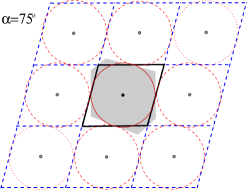
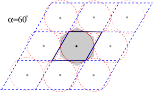
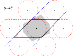
Figure 1: The pattern in CMB correlation in a multi-connected universe, ${\cal M}\equiv{\cal M}^{u}/\Gamma$ is related to the distribution of ‘images’ of the sphere of last scattering (SLS) on the universal cover. The three figures illustrate this for three values of $\alpha=45^{\circ},60^{\circ},75^{\circ}$ in a squeezed torus. The solid parallelepiped is the fundamental domain and the dashed show its images tessellate,${\cal M}^{u}$. The solid circle is the SLS and dashed/dotted ones are its images. In each case, the radius of SLS is equal to the inradius, $R_{<}$ of ${\cal M}$. The shaded polygon is the Dirichlet domain (DD). The closest SLS images which determine the DD are dashed (others are dotted). Note the hexagonal shape of DD when $\alpha\neq\pi/2$ and is equal sided for $\alpha=\pi/3$. For smaller $\alpha$, the DD approximates an elongated cuboid.

The set of measures $\kappa_{\ell}$ of statistical isotropy violation is defined as

$$\kappa_{\ell}=\int\!\!d\Omega\!\!\int\!\!d\Omega^{\prime}\left[\frac{(2\ell+1)}{8\pi^{2}}\!\!\int d{\mathcal{R}}\chi_{\ell}({\mathcal{R}})C({\mathcal{R}}\hat{q},{\mathcal{R}}\hat{q}^{\prime})\right]^{2}\!\!\!\!,$$ (1)

where $C({\mathcal{R}}\hat{q},\,{\mathcal{R}}\hat{q}^{\prime})$ is the two point correlation between ${\mathcal{R}}\hat{q}\,$ and ${\mathcal{R}}\hat{q}^{\prime}$ obtained by rotating $\hat{q}$ and $\hat{q}^{\prime}$ by an element ${\mathcal{R}}$ of the rotation group us_apj . The measures $\kappa_{\ell}$ involve angular average of the correlation weighed by the characteristic function of the rotation group $\chi_{\ell}({\mathcal{R}})=\sum_{M}D_{MM}^{\ell}({\mathcal{R}})$ where $D_{MM^{\prime}}^{\ell}$ are the Wigner D-functions Var . When SI holds $C({\mathcal{R}}\hat{q},\,{\mathcal{R}}\hat{q}^{\prime})\,=\,C(\hat{q},\,\hat{q}^{\prime})$ is invariant under rotation, and eq. (1) gives $\kappa_{\ell}=\kappa_{0}\,\delta_{\ell 0}$ due to the orthonormality of $\chi_{\ell}({\mathcal{R}})$. Hence, non-zero $\kappa_{\ell}$ for $\ell>0$ measure violation of statistical isotropy.

The measure $\kappa_{\ell}$ has a clear interpretation in harmonic space. The two point correlation $C(\hat{q},\,\hat{q}^{\prime})$ can be expanded in terms of the orthonormal set of bipolar spherical harmonics as

$$C(\hat{q},\,\hat{q}^{\prime})\,=\,\sum_{ll^{\prime}\ell M}A_{ll^{\prime}}^{\ell M}\{Y_{l}(\hat{q})\otimes Y_{l^{\prime}}(\hat{q}^{\prime})\}_{\ell M}\,,$$ (2)

where $A_{ll^{\prime}}^{\ell M}$ are the coefficients of the expansion. These coefficients are related to ‘angular momentum’ sum over the covariances $\langle a_{lm}a^{*}_{l^{\prime}m^{\prime}}\rangle$ as

$$A_{ll^{\prime}}^{\ell M}=\sum_{mm^{\prime}}\langle a_{lm}a^{*}_{l^{\prime}m^{\prime}}\rangle\,\,(-1)^{m^{\prime}}\mathfrak{C}^{\ell M}_{lml^{\prime}-m^{\prime}}\,,$$ (3)

where $\mathfrak{C}^{\ell M}_{lml^{\prime}m^{\prime}}$ are Clebsch-Gordan coefficients Var . When SI holds $\langle a_{lm}a^{*}_{l^{\prime}m^{\prime}}\rangle=C_{l}\delta_{ll^{\prime}}\delta_{mm^{\prime}}$, implying $A_{ll^{\prime}}^{\ell M}=(-1)^{l}C_{l}(2l+1)^{1/2}\,\delta_{ll^{\prime}}\,\delta_{\ell 0}\,\delta_{M0}$. $A_{ll}^{00}$ represent the statistically isotropic part of a general correlation function. The bipolar functions transform just like ordinary spherical harmonic function $Y_{LM}$ under rotation Var . Substituting the expansion eq. (2) into eq. (1) we can show that $\kappa_{\ell}=\sum_{ll^{\prime}M}|A_{ll^{\prime}}^{\ell M}|^{2}$ is positive semidefinite and is also given by

$$\kappa_{\ell}=\frac{2\ell+1}{8\pi^{2}}\!\!\int\!\!d{\mathcal{R}}\chi_{\ell}({\mathcal{R}})\sum_{lml^{\prime}m^{\prime}}\langle a_{lm}a^{*}_{l^{\prime}m^{\prime}}\rangle\langle a_{lm}a^{*}_{l^{\prime}m^{\prime}}\rangle^{\mathcal{R}}\!\!,$$ (4)

where $\langle\ldots\rangle^{\mathcal{R}}$ is computed in a frame rotated by ${\mathcal{R}}$ us_apj .

The compact spaces with Euclidean geometry (zero curvature) have been completely classified. In three dimensions, there are known to be six possible topologies that lead to orientable spaces  costop ; wol94vin93 . The simple flat torus, ${\cal M}=T^{3}$, is obtained by identifying the universal cover ${\cal M}^{u}={\cal E}^{3}$ under a discrete group of translations along three non-degenerate axes, ${\mathbf{s}_{1},\mathbf{s}_{2},\mathbf{s}_{3}}$: ${\mathbf{s}_{i}}\to{\mathbf{s}_{i}}+{\mathbf{n}}L_{i}$, where $L_{i}$ is the identification length of the torus along $s_{i}$ and ${\bf n}$ is a vector with integer components. In the most general form, the fundamental domain (FD) is a parallelepiped defined by three sides $L_{i}$ and the three angles $\alpha_{i}$ between the axes (We call it squeezed torus). If ${\mathbf{s}_{i}}$ are orthogonal then one gets cuboidal FD, which for equal $L_{i}$ reduces to the cubic torus. The cuboid and squeezed spaces which can be obtained by a linear coordinate transformation ${\cal L}$ on cubic torus bow_fer02 can have distinctly different global symmetry .

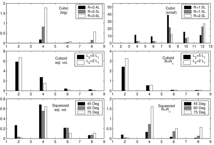
Figure 2: The $\kappa_{\ell}$ spectra for flat tori models are plotted. The top row panels are for cubic tori spaces. The left panel shows spaces of volume, $V_{\cal M}$, larger than the volume $V_{*}$ contained in the sphere of last scattering (SLS) with $V_{\cal M}/V_{*}=3.7,1.9,1.1$, respectively. The right panel shows small spaces with $V_{\cal M}/V_{*}=0.24,0.07,0.03$, respectively. Note that $\kappa_{2}=0$ for cubic tori. The middle panels consider cuboid tori with $1:5$ and $1:2$ ratio of identification lengths. The bottom panels show $\kappa_{\ell}$ for equal-sided squeezed tori with $\alpha=45^{\circ},60^{\circ}$ and $75^{\circ}$. In the middle and bottom rows, the right panels show the case when radius of SLS, $R_{*}=R_{<}$ the inradius of the space. Here, the SLS just touches its nearest images (see Fig. 1) which is at the threshold where CMB anisotropy is multiply imaged for larger $R_{*}$. The cases in the left panels of lower two rows have $V_{\cal M}/V_{*}=1$ and are at the divide between large and small spaces.

We restrict attention to the case where CMB anisotropy arises entirely at the sphere of last scattering (SLS) of radius $R_{*}$ (nearly equal to observable horizon). Invoking method of images, the CMB correlation pattern on the SLS is known to be dictated by the distribution of nearest ‘images’ of the SLS on the universal cover bps . The correlations are distorted even when the SLS and its images do not intersect ($R_{*}<R_{<}$). When SLS intersects its images the CMB sky is multiply imaged in characteristic correlation pattern of pairs of circles circles . Fig. 1 illustrates the role of the nearest SLS images and related DD in defining the principal directions in the correlation for a few cases.

We compute $C({\hat{q},\hat{q}^{\prime}})$ for CMB anisotropy in torus space using regularized method of images bps . We can compute the $\kappa_{\ell}$ in real space using eq. (1) or from $A_{ll^{\prime}}^{\ell M}$ using eq. (3) in harmonic space. Fig. 2 plots the $\kappa_{\ell}$ spectrum for a number of cubic, cuboidal and squeezed torus spaces. We find the following interesting results :

i. $\kappa_{\ell}=0$ for odd $\ell$ for all torus models. This does not hold for compact space of non-zero curvature, e.g., compact hyperbolic spaces.

ii. For cubic torus $\kappa_{2}=0$. $\kappa_{2}$ is non-zero for cuboidal and squeezed torus. This is a clear signature of non-cubic torus where the DD differs from the FD and has more than three principle axes.

iii. For equal-sided squeezed torus, $\kappa_{4}$ , decreases as $\alpha$ decreases from $90^{\circ}$ to $60^{\circ}$ as $R_{<}$ increases. For $\alpha<60^{\circ}$ sharply increases with decreasing $\alpha$ as $R_{<}$ decreases sharply bow_fer02 .

iv. $\kappa_{2}=0$ increases monotonically as $\alpha$ decreases from $90^{\circ}$. The trend is well fit by eq. (13).

v. The peak of $\kappa_{\ell}$ shifts to larger $\ell$ for small spaces.

The results can be understood using the leading order terms of the correlation function in a torus where $\kappa_{\ell}$ can be calculated analytically. For brevity, we outline the steps for the cubic torus. The results for cuboid and squeezed case is readily obtained using the transformation ${\mathcal{L}}$. Here we list only the results leaving details of the calculation to a more comprehensive publication us_inprep .

The spatial correlation function of gravitational potential in the periodic box implied by the $T^{3}$ topology with cubic fundamental domain is

$$\xi_{\Phi}({\bf x,x^{\prime}})=L^{-3}\sum_{{\bf n}}P_{\Phi}(k_{\bf n})\,\,{\mathrm{e}}^{-i\frac{2\pi{\bf n}}{L}\cdot({\bf x}-{\bf x}^{\prime})},$$ (5)

where ${\bf n}$ is 3-tuple of integers, $k^{2}_{\bf n}=(2\pi/L)^{2}({\bf n}\cdot{\bf n})$, and the term with ${\bf n}\cdot{\bf n}=0$ is excluded from the summation. For Naive Sachs-Wolfe CMB anisotropy arising at the SLS ( $\Delta T=1/3\Phi$), the correlation function, $C(\hat{q},\hat{q}^{\prime})$ is given by the spatial correlation of $\Phi$ at points on the SLS along the two directions $\hat{q}$ and $\hat{q}^{\prime}$ as

$$C({\hat{q},\hat{q}^{\prime}})=L^{-3}\sum_{{\bf n}}P_{\Phi}(k_{\bf n})\,\,{\mathrm{e}}^{-i\pi(\epsilon_{\hat{q}}{\bf n}\cdot{\hat{q}}-\epsilon_{\hat{q}^{\prime}}{\bf n}\cdot{\hat{q}}^{\prime})},$$ (6)

where the small parameter $\epsilon_{\hat{q}}\leq 1$ is the physical distance to the SLS along $\hat{q}$ in units of $L/2$ (more generally, $\bar{L}/2$ where $\bar{L}=(L_{1}L_{2}L_{3})^{1/3}$). Contribution to $C({\hat{q},\hat{q}^{\prime}})$ from large wavenumbers, $|\bf n|\epsilon\gg 1$ is expected to be approximately statistically isotropic. The SI violation is found in the low wavenumbers.

When the SLS is contained with the fundamental domain around the observer, i.e., the CMB anisotropy is not multiply imaged on the sky, $\epsilon=2R_{*}/L$ is a constant. When $\epsilon$ is a small constant, the leading order terms in the correlation function eq. (6) can be readily obtained in power series expansion in powers of $\epsilon$. For the lowest wavenumbers $|{\mathbf{n}}|^{2}=1$ in a cuboid FD torus

$$C({\hat{q},\hat{q}^{\prime}})\approx 2\sum_{i}P_{\Phi}({2\pi}/{L_{i}})\cos(\pi\epsilon\beta_{i}\Delta q_{i}).$$ (7)

where $\Delta q_{i}$ are the components of ${\mathbf{\Delta}q}=\hat{q}-\hat{q}^{\prime}$ along the three axes of the torus and $\beta_{i}=\bar{L}/L_{i}$. Only even powers of $\epsilon\Delta q_{i}$ are present in the expansion eq. (7). This holds for the terms from higher wavenumbers ($|{\mathbf{n}}|^{2}=2$ or $3$) and explains the strictly zero $\kappa_{\ell}$ for odd $\ell$ us_inprep .

In a cubic (equal sided) torus, up to the leading order SI violating term, the correlation is

$$C({\hat{q},\hat{q}^{\prime}})\approx C_{0}\left[1-\epsilon^{2}\,|{\mathbf{\Delta}q}|^{2}+3\,\epsilon^{4}\,\sum_{i=1}^{3}(\Delta q_{i})^{4}\right].$$ (8)

We retain the $\epsilon^{4}$ term since the term at $\epsilon^{2}$ is explicitly rotationally invariant, hence does not contribute to the violation of SI. The non-zero $\kappa_{\ell}$ can be analytically computed to be

$$\frac{\kappa_{0}}{C_{0}^{2}}\, = \,\pi^{2}(1-4\epsilon^{2}+\frac{368}{15}\epsilon^{4}-\frac{288}{5}\epsilon^{6}+\frac{20736}{125}\epsilon^{8})$$

$$\frac{\kappa_{4}}{C_{0}^{2}}\, = \,\frac{12288\pi^{2}}{875}\epsilon^{8}$$ (9)

The first non zero $\kappa_{\ell}$ in cubic (equal-sided) torus occurs at $\ell=4$. $\kappa_{4}\sim\epsilon^{8}$ falls off rapidly as $\epsilon\rightarrow 0$ for large spaces.

For the cuboidal (unequal-sided) torus, the correlation violates SI at order $\epsilon^{2}$

$$C({\hat{q},\hat{q}^{\prime}})\approx C_{0}\left[1-\epsilon^{2}\sum_{i=1}^{3}\beta_{i}^{2}\,(\Delta q_{i})^{2}\right].$$ (10)

The non zero $\kappa_{\ell}$ corresponding to the correlation eq. (10) are

$$\frac{\kappa_{0}}{C_{0}^{2}}\, = \,\pi^{2}(1-\frac{4}{3}\beta^{2}\epsilon^{2}+\frac{16}{27}\beta^{4}\epsilon^{4})$$

$$\frac{\kappa_{2}}{C_{0}^{2}}\, = \,\frac{64\pi^{2}}{135}\left[\beta^{4}-3(\beta_{1}^{2}\beta_{2}^{2}+\beta_{1}^{2}\beta_{3}^{2}+\beta_{2}^{2}\beta_{3}^{2})\right]\epsilon^{4}$$ (11)

where $\beta^{2}=\sum_{i=1}^{3}\beta_{i}^{2}$. The $\kappa_{2}\sim\epsilon^{4}$ signal falls off slower than the $\kappa_{4}$ signal in cubic space for large spaces ($\epsilon\rightarrow 0$).

For the squeezed torus, the linear transformation can be applied to obtain the expansion up to the leading order SI violating term. For simplicity, we restrict to equal sided squeezed torus with one non-orthogonal pair of axes (${\mathbf{s}_{1}}\cdot{\mathbf{s}_{2}}=\cos\alpha$). The leading order approximation to correlation $C({\hat{q},\hat{q}^{\prime}})$ has the form

$$C_{0}\left[1-\epsilon^{2}\frac{|{\mathbf{\Delta}q}|^{2}+2\cos{\alpha}\Delta q_{1}\Delta q_{2}+\cos^{2}{\alpha}\Delta q_{3}^{2})}{3\sin^{2}{\alpha}}\right].$$ (12)

The corresponding $\kappa_{\ell}$ spectrum is

$$\frac{\kappa_{0}}{C_{0}^{2}} = \pi^{2}[1+8\sin^{2}\alpha+\frac{64}{27}\cos^{4}\alpha-12\epsilon^{2}(1-\frac{16}{27}\cos^{2}\alpha)]$$

$$\frac{\kappa_{2}}{C_{0}^{2}}\, = \,\frac{64\pi^{2}}{135}(\cos^{4}\alpha+3\,\epsilon^{4}\frac{\cos^{2}{\alpha}}{\sin^{4}\alpha}).$$ (13)

The expression for $\kappa_{2}$ explains point (iv) regarding $\kappa_{\ell}$. Interestingly, a residual $\kappa_{2}$ remains even for very large space ($\epsilon\rightarrow 0$).

Preferred directions and statistically anisotropic CMB anisotropy have been discussed in literature fer_mag97bun_scot00 . We compute SI violation of the CMB anisotropy due to cosmic topology quantified in terms of the recently proposed $\kappa_{\ell}$ spectrum us_apj . We interpret generic features of $\kappa_{\ell}$ spectrum arising from the shape of the Dirichlet domain as well as through analytic results for leading order approximation to the correlation. These results help interpret observed non-zero $\kappa_{\ell}$ and discriminate between different topologies of the universe. When CMB anisotropy is multiply imaged, the $\kappa_{\ell}$ spectrum corresponds to a correlation pattern of matched pairs of circles circles . $\kappa_{\ell}$ have an advantage of being insensitive to the overall orientation of the correlation features. Also $\kappa_{\ell}$ are sensitive to SI violation even when CMB is not multiply imaged. The $A^{\ell M}_{ll^{\prime}}$ signature, which was not discussed here, contains more details of the SI violation us_inprep .

We study a new measure of SI violation. A companion paper describes the estimation of $\kappa_{\ell}$ from a CMB map us_apj . Before ascribing the detected breakdown of statistical anisotropy to cosmological or astrophysical effects, one must carefully account for and model out other mundane sources of statistical anisotropy in real data, such as, incomplete and non-uniform sky coverage, beam anisotropy, foreground residuals and statistically anisotropic noise. These observational artifacts will be discussed in future publications.

References

(1) A. Hajian & T. Souradeep, preprint,
astro-ph/0308001.
(2) G. F. R. Ellis, Gen. Rel. Grav. 2, 7,(1971); M.
Lachieze-Rey & J. -P. Luminet, Phys. Rep. 25, 136, (1995);
J. Levin, Phys. Rep. 365, 251, (2002); G. Starkman, Class.
Quantum Grav. 15, 2529, (1998).
(3) J. R. Bond, D. Pogosyan & T. Souradeep, Class. Quant.
Grav. 15, 2671, (1998); ibid. Phys. Rev. D
62,043005, (2000);ibid.,043006, (2000); T. Souradeep, in
‘The Universe’, ed. N. Dadhich & A. Kembhavi (Kluwer, 2000).
(4) A. A. Starobinsky, JETP Lett. 57, 622,
(1993); I. Y. Sokolov, JETP Lett. 57, 617, (1993); D. Stevens,
D. Scott & J. Silk, Phys. Rev. Lett. 71, 20, (1993); A. de
Oliveira Costa & G. F. Smoot, Ap. J. 448 477, (1995); A. de
Oliveira Costa, G. F. Smoot & A. A. Starobinsky, Ap. J. 468,
457, (1996); J. Levin, E. Scannapieco, J. Silk, Phys. Rev. D58,
103516, (1998).
(5) R. Bowen, P.G. Ferreira, Phys. Rev. D66,
041302, (2002).
(6) D. A. Varshalovich, A. N. Moskalev, V. K. Khersonskii,
Quantum Theory of Angular Momentum (World Scientific 1988).
(7) J. A. Wolf, Space of Constant Curvature (5th
ed.), (Publish or Perish, Inc., 1994); E. B. Vinberg, Geometry II – Spaces of constant curvature, (Springer-Verlag,
1993).
(8) Hajian, A. & Souradeep, T., in preparation.
(9) N.J. Cornish, D.N. Spergel & G. D. Starkman,
Class. Quantum Grav., 15, 2657, (1998).
(10) P. G. Ferreira & J. Magueijo, Phys.
Rev. D56, 4578, (1997); E. Bunn & D. Scott, M.N.R.A.S., 313,