Galactic Foreground Constraints from the Python V Cosmic Microwave Background Anisotropy Data

Abstract

We constrain Galactic foreground contamination of the Python V cosmic microwave background anisotropy data by cross correlating it with foreground contaminant emission templates. To model foreground emission we use 100 and 12 $\mu$m dust templates and two point source templates based on the PMN survey. The analysis takes account of inter-modulation correlations in 8 modulations of the data that are sensitive to a large range of angular scales and also densely sample a large area of sky. As a consequence the analysis here is highly constraining. We find little evidence for foreground contamination in a analysis of the whole data set. However, there is indication that foregrounds are present in the data from the larger-angular-scale modulations of those Python V fields that overlap the region scanned earlier by the UCSB South Pole 1994 experiment. This is an independent consistency cross-check of findings from the South Pole 1994 data.

1 Introduction

While cosmic microwave background (CMB) anisotropy data have started to provide interesting constraints on cosmological parameters (see, e.g., Podariu et al. 2001; Page 2002; Mukherjee et al. 2002b, 2003; Benoît et al. 2003; Ruhl et al. 2002; Kuo et al. 2002; Slosar et al. 2002 for recent results, and Peebles & Ratra 2003 for a review), Galactic emission foreground contaminants in them are still not well understood. Robust constraints on cosmological parameters from these data require a better understanding of the effect of these contaminants.

In this paper we study foreground contaminants in the Python V (hereafter PyV) CMB anisotropy data. Python V is the latest of the Python experiments at the South Pole. Coble et al. (1999, 2003) describe the PyV experiment, observations, and data reduction. Dragovan et al. (1994), Ruhl et al. (1995), and Platt et al. (1997) describe Python I–III and Rocha et al. (1999) and Mukherjee et al. (2003) derive constraints on cosmological parameters from these data. Coble et al. (2003) also describe the procedure used to create maps of the sky with PyV and Python III data; these maps were compared to infer consistency and indirectly deduce the lack of significant foreground contamination in these data.

The PyV data are acquired at a frequency of $\sim 40$ GHz. Two regions of sky covering 598 deg² in the southern hemisphere were observed (the “main PyV” region and a smaller region, the fields labelled ‘sa’, ‘sb’, and ‘sc’ in Coble et al. 2003, that encompasses the region scanned earlier by the UCSB South Pole 1994 experiment — hereafter the “SP94 overlap” region). 690 fields were scanned in all (345 effective fields were scanned with 2 detector feeds separated by $2.\!\!^{\circ}8$ in azimuth on the sky) with an asymmetric Gaussian beam of FWHM $0.\!\!^{\circ}94\times 1.\!\!^{\circ}02$. Once the telescope was positioned on each field, the chopper smoothly scanned in azimuth with a throw of 17^∘, 128 samples were recorded in each chopper cycle, and 164 chopper cycles of data were taken of a given field. The densely sampled data were then modulated in software using the first eight cosine harmonics of the chopper cycle (hereafter modulations — or in Tables mods — 1-8). The modulations approach used has the advantage of filtering out some of the contaminants in the time stream, and also provides a rapid means of compressing a large amount of data into a more manageable size. All the modulations, other than the first, were apodized by a Hann window to reduce ringing in multipole space and down weight data taken during chopper turnaround. The resulting data are sensitive to angular scales corresponding to multipole moments ranging from $l\sim 40$ to $l\sim 260$. More details about the particular observing strategy employed and results found, such as the angular power spectrum of the data, may be found in Coble et al. (2003); see Souradeep & Ratra (2001) for details about the window functions.

For this foregrounds analysis, we follow the general method outlined for example in Hamilton & Ganga (2001) and Mukherjee et al. (2002a), doing a multi-modulation analysis here rather than the multi-(frequency) channel analysis discussed in these papers. In doing so we extend the preliminary estimate presented in Coble et al. (1999). Here we use the technique of Souradeep & Ratra (2001) to account for correlations between modulations, in data that are sensitive to a substantial range of angular scales, as well as compare to what has been found from the SP94 experiment (Gundersen et al. 1995; Ganga et al. 1997) data about foreground contamination in part of the PyV region (Hamilton & Ganga 2001; Mukherjee et al. 2002a).

CMB data have previously been correlated with foreground templates (DMR: Kogut et al 1996a, 1996b; 19GHz: de Oliveira-Costa et al. 1998; Saskatoon: de Oliveira-Costa et al. 1997; OVRO: Leitch et al. 1997, Mukherjee et al. 2002a; SP94: Hamilton & Ganga 2001, Mukherjee et al. 2002a; Tenerife: de Oliveira-Costa et al. 1999, 2002, Mukherjee et al. 2001; QMAP: de Oliveira-Costa et al. 2000; MAX: Lim et al. 1996, Ganga et al. 1998; and Boomerang: Masi et al. 2001). Correlations between CMB data and infra-red emission seem to be roughly consistent with free-free emission, spectrally, over a wide range of frequencies (10 to 90 GHz) and angular scales ($7^{\circ}$ to $7^{\prime}$), with some evidence for a contribution from spinning dust emission with a peak around 15 to 20 GHz. In general though the contamination from foregrounds has not been found to be large in any experiment, but on the detail level residual foregrounds can cause problems with parameter estimation and non-Gaussianity tests for high precision CMB data.

To model diffuse Galactic emission, we use the 100 $\mu$m IRAS+DIRBE map (Schlegel, Finkbeiner, & Davis 1998) as a tracer of thermal emission from interstellar dust, and the 12 $\mu$m map (D. Finkbeiner, private communication, 2000) as a tracer of emission from ultra-small dust grains. Emission from small dust grains is still under study (Finkbeiner et al. 2002). Such grains may contribute significantly at microwave frequencies according to a model by Draine & Lazarian (1998a,b), and this has been reviewed from the CMB data point of view by Kogut (1999) and Draine & Lazarian (1999). The Haslam 408 MHz map (Haslam et al. 1981) of synchrotron emission was not used as it does not have enough resolution for all the modulations of the PyV experiment to be simulated on it. At the same time synchrotron emission is not likely to contribute significantly at 40 GHz. We have tried to use the SHASSA $H_{\alpha}$ data (Gaustad et al. 2001) as a tracer of free-free emission, but found that the template has insufficient resolution for our purpose.

We also use two point source templates created from the PMN survey (Wright et al. 1994). The one called PMN has been converted to $\delta T_{CMB}$ (equivalent temperature fluctuations in the CMB at 40 GHz) using the spectral indices given in the survey, while the one called PMN0 is converted to a flux at 40 GHz assuming a flat spectrum extrapolated from the flux measurement at 4.85 GHz. The assumption of a flat spectrum is conservative in that it is likely to overestimate the flux at 40 GHz. Neither case is correct, since spectral indices have not been measured for all of the sources, in which case a flat spectrum is assumed. The two cases cover a reasonable range of possibilities. These templates were also used in the preliminary foreground analysis of Coble et al. (1999).

Each of the Galactic emission maps have been converted into a template for cross correlation with the PyV data by simulating the PyV observing strategy on it, taking account of the asymmetric beam. Since a chopper synchronous offset and a ground shield offset were removed from the data, we account for this by adding the chopper synchronous offset and ground shield constraint matrices to the noise matrix and marginalizing over them in the analysis. The CMB theory covariance matrix is modelled using a spatially-flat cosmological constant dominated CDM model with non-relativistic matter density parameter $\Omega_{0}=0.3$, scaled baryonic matter density parameter $\Omega_{B}h^{2}=0.021$ (here $h$ is the present value of the Hubble parameter in units of 100 km s^-1 Mpc^-1), and age $t_{0}=14$ Gyr (Ratra et al. 1999a) with the CMB anisotropy normalized to a quadrupole moment amplitude $Q_{\rm rms-PS}=20$ $\mu$K.

2 Correlations

2.1 Method

We follow the general method outlined for example in Hamilton & Ganga (2001) and Mukherjee et al. (2002a), doing a multi-modulation analysis here rather than the multi-(frequency) channel analysis discussed in these papers. The method assumes that the data are a linear combination of CMB anisotropies and foreground components,

$$y=aX+x_{\rm CMB}+n.$$ (1)

Here $y$ is a $n_{\rm mod}\times N$ element vector containing the data, $n$ is the corresponding noise vector, $x_{\rm CMB}$ is the CMB signal, and $X$ is a $(n_{\rm mod}\times N)\times n_{\rm mod}$ element matrix containing the simulated foreground template, $N$ being the number of data points per modulation and $n_{\rm mod}$ being the number of modulations. In a given column $X$ contains mostly zeros except for the rows corresponding to that modulation, where it contains the simulated template signal. The vector $a$ contains $n_{\rm mod}$ elements that represent the amplitude of the correlated foreground signal. If the noise and CMB anisotropies are uncorrelated Gaussian distributed variables with zero mean, minimizing $\chi^{2}$ leads to a best fit estimate of

$$\hat{a}=[X^{T}C^{-1}X]^{-1}X^{T}C^{-1}y,$$ (2)

where $C$ is the $(n_{\rm mod}\times N)\times(n_{\rm mod}\times N)$ element total covariance matrix (sum of the theory covariance matrix that models the CMB signal, the noise covariance matrix, and any constraint matrices). The vector $\hat{a}$ then contains the best estimate for the correlation slopes for the corresponding template for all modulations, given all information about inter-modulation correlations. The matrix

$$\Sigma=\langle\hat{a}^{2}\rangle-\langle\hat{a}\rangle^{2}=[X^{T}C^{-1}X]^{-1},$$ (3)

is its covariance matrix. The rms amplitudes of temperature fluctuations in the data that results from the correlation is $\Delta T=(\hat{a}\pm\delta\hat{a})\sigma_{\rm{fore}}$, where $\sigma_{\rm{fore}}$ contains the rms deviations of the corresponding foreground template in the different modulations.

The method assumes that our foreground emission maps are good enough to model the foregrounds in the data accurately in all the different modulations, at a frequency different from that of the original foreground emission map, and that eq. (1) explains all the structure in all modulations of the data. If we further assume that the ratio of the signal in the data and that in the foreground template is the same for all the modulations, then a net correlation slope can be found using

$$\bar{a}=\frac{\rm{Total}(\Sigma^{-1}a)}{\rm{Total}(\Sigma^{-1})}.$$ (4)

Here Total denotes the sum of all elements of a matrix or vector. This is thus a weighted average taking account of correlations between the $a$ values of the different modulations. We may choose not to treat all modulations the same (see discussion in $\S$ 2.3). The error bar on $\bar{a}$ is $\sqrt{({\rm Total}(\Sigma^{-1}))^{-1}}$.

2.2 Results

The correlation slopes obtained from a complete inter-modulation analysis, using all the PyV data points, for each foreground emission template individually, are given in Table 1 (top panel). We do not find any significant correlation. The net correlation slopes (i.e., the weighted mean of the correlation slopes given in the table, taking cross-modulation correlations into account) are not significant, with two standard deviation upper limits of 34 $\mu$K(MJy/sr)^-1, 110 $\mu$K(MJy/sr)^-1, 156 $\mu$K/$\mu$K, and 897 $\mu$K(MJy/sr)^-1, for the 100 $\mu$m, the 12 $\mu$m, the PMN, and the PMN0 templates, respectively. These limits on 100 $\mu$m and PMN0 correlation slopes compare well with those of Table 2 of Coble et al. (1999). (There are some errors in the PMN correlation slopes of Table 2 and the rms values in Table 3 of Coble et al. 1999.) The upper limits obtained from using all modulations of the data together are given in Table 3.

The results of repeating this analysis for just the SP94 overlap region are also given in Table 1 (bottom panel). The uncertainties in the estimated correlation slopes are higher here, with the number of data points down by a factor of almost 8 (the time spent observing this region was less than 1:8 of the total observing time), but the level of associated temperature fluctuations are relatively higher, at least for the 100 $\mu$m template. As seen from Tables 2 and 3, the rms of the data and the 100 $\mu$m template are higher in this patch of sky. Again, no significant correlations are found. The weighted correlation coefficient between foreground emission templates is given by $\Sigma_{ij}^{-1}(\Sigma_{ii}^{-1}\Sigma_{jj}^{-1})^{-0.5}$ (de Oliveira-Costa et al. 1999). The 100 and 12 $\mu$m templates and the PMN and PMN0 templates are found to have significant weighted correlation coefficients in this region of sky, with the correlation reducing somewhat, from 0.7 to 0.5, with increasing modulation for the two dust templates, while it remains steady at about 0.85 for the two point source templates. (These templates are much less like each other when all the PyV fields are considered.) Yet when all modulations of the data are analysed together, joint template fits do not detect any correlations. The net correlation slopes obtained from a complete inter-modulation analysis of the SP94 overlap region are not significant, with 2 $\sigma$ upper limits of 69 $\mu$K(MJy/sr)^-1, $1027$ $\mu$K(MJy/sr)^-1, $603$ $\mu$K/$\mu$K, and $2198$ $\mu$K(MJy/sr)^-1, for the 100 $\mu$m, the 12 $\mu$m, the PMN, and the PMN0 templates, respectively. The upper limits obtained from using all modulations of the data together are given in Table 3.

2.3 Low $l$ Modulations

As seen from Table 2, the signal in the foreground templates falls more steeply with increasing modulation number than does the data. So the case here, of fitting for several modulations simultaneously, is somewhat different from the case of fitting multi-frequency data: if a certain foreground is present in the data, picking it out in the higher modulations will be harder. But the cumulative effect of the other modulations is significant on the estimated correlation slope for any modulation; Figure 2 of Coble et al. (1999) shows how much the CMB signal in different modulations overlap. Hence simultaneously fitting for the correlation slopes in all the modulations of the data may not be the most appropriate thing to do. It is also important to note that the foregrounds may not have been accurately modelled in the higher modulations because of insufficient resolution (given the dense sampling in the data). There may also be different kinds of unmodelled or incorrectly modelled foregrounds/errors in different modulations. Hence it is useful to also look at the results from analysing say the first three modulations together, because across these modulations the data and the foreground signal seem to be roughly similar as regards rms values, or each modulation individually, at the cost of increased uncertainty in the estimates.

If we look at only the first modulation in the SP94 overlap region, we find a 1.8 $\sigma$ correlation slope of $80\pm 45$ $\mu$K(MJy/sr)^-1 ($36\pm 21$ $\mu$K) for the 100 $\mu$m template (Table 4). For the 12 $\mu$m template the correlation found is just less than a sigma, but here the two dust templates have a weighted correlation coefficient of 0.65, and performing a joint correlation of the data with these two templates results in a 1.9 $\sigma$ correlation slope of $115\pm 60$ $\mu$K(MJy/sr)^-1 ($52\pm 27$ $\mu$K) for the 100 $\mu$m template at the cost of a 1 $\sigma$ negative correlation with the 12 $\mu$m template. This may be the signal found in the foregrounds analysis of the SP94 data (Hamilton & Ganga 2001; Mukherjee et al. 2002a; for earlier qualitative indications see Ganga et al. 1997; Ratra et al. 1999b). While there a detection was aided by the presence of 7 frequency channels, here the error bars for the individual modulation correlations are large. This could be just a chance correlation on the other hand, and the probability of that is reflected in the significance of the result. It might also be relevant to note here that the SP94 data was only one dimensional while here the PyV ‘sa’, ‘sb’, and ‘sc’ data are essentially two dimensional.

If we look at only the second modulation by itself, the correlation slopes are as shown in Table 4, and even though the correlation coefficient between the 12 and 100 $\mu$m templates is 0.70 nothing is gained by a joint fit this time.

In the first two modulations together some correlation with the 100 $\mu$m template is detected consistent with the above estimates. When the first three modulations are correlated simultaneously, a 1.6 $\sigma$ correlation slope of $58\pm 36$ $\mu$K(MJy/sr)^-1 ($25\pm 16$ $\mu$K) is found with the 100 $\mu$m template in the first modulation and a 1 $\sigma$ $710\pm 695$ $\mu$K(MJy/sr)^-1 ($14\pm 14$ $\mu$K) correlation is found with the 12 $\mu$m template in the second modulation. The correlation coefficient between the templates is high and correlations of similar significance are found in the same modulations when the two templates are analysed jointly.

Regarding the point source templates, nothing significant shows up in an individual template analysis (Table 4). When analysing the first two modulations together the two point source templates have a correlation coefficient of 0.8 and a correlation slope of $6555\pm 4994$ $\mu$K(MJy/sr)^-1 ($28\pm 21$ $\mu$K) at 1.3 $\sigma$ is found with the PMN0 template in modulation 1 at the cost of a 1 $\sigma$ negative correlation with the PMN template in the same modulation. When analysing the first three modulations together the point source templates have a high correlation coefficient and a 1.2 $\sigma$ correlation of $5625\pm 4498$ $\mu$K(MJy/sr)^-1 ($24\pm 19$ $\mu$K) is found with the PMN0 template in modulation 1 at the cost of a $-1$ $\sigma$ correlation with the PMN template in the same modulation.

When all the PyV fields are taken together (690 in each modulation), a 1 $\sigma$ correlation with the 100 $\mu$m template shows up in the first modulation (when the first modulation is analysed by itself, or jointly with the second, or jointly with the second and third), and a 1 $\sigma$ correlation with the PMN0 template shows up in the first modulation when it is analysed together with the second modulation and jointly with the PMN template. The uncertainty in the correlation slopes with the point source templates is lowest in the third and fourth modulations, but nothing significant shows up when these modulations are analysed separately. Hence consistent correlations (in the low-$l$ modulations and at low significance) are seen even when both the PyV regions are analysed together.

2.4 Summary

When all the modulations of the data are analysed together, no significant correlations are found, in the whole PyV data set or in the SP94 overlap region. These results are summarized in Table 3 and plotted in Figure 1.

We have discussed the motivations for looking at individual modulations separately, and we find some indication of foregrounds in the low $l$ modulations. Correlation slopes for some of these low $l$ modulations are summarized in Table 4. We see that greater than 1 $\sigma$ correlations show up in the SP94 overlap region with the 100 $\mu$m template in particular, but also with the 12 $\mu$m template and the PMN0 template in some modulations in a joint modulation analysis of a few modulations. And consistent correlations are seen when all the PyV data fields are analysed together.

We note that according to the foreground model discussed for example in Mukherjee et al. (2002a), if the 100 $\mu$m correlations are from both free-free emission and spinning dust emission, then by 40 GHz the contribution from spinning dust emission (as traced by the 12 $\mu$m template) may have again dropped below that from free-free (the frequency at which spinning dust emission peaks depends on the details of the spinning dust emission model and this can also vary from region to region), so that we would expect 100 $\mu$m correlations to be more significant than 12 $\mu$m correlations at this frequency (see Figure 1$a$). However, given the error bars (the numbers in Table 4), we do not expect to see significant correlations in the PyV data (see Figure 1).

3 Conclusion

Using the method of cross correlating CMB anisotropy data with foreground contaminant emission templates, we find little evidence for foreground contamination in the whole PyV region when analysing all modulations of the data together. There is however indication of foreground contamination in the low-$l$ modulations of the PyV fields that cover the region scanned earlier by the SP94 experiment, consistent with results from the SP94 data. This is a valuable test, indicating consistency between results found using data from two different experiments. Given the uncertainties, our findings are not inconsistent with the two component dust-correlated (free-free and spinning dust) foreground emission model that other data sets tentatively seem to point to (Mukherjee et al. 2002a).

We thank D. Finkbeiner for the 12 $\mu$m dust map and E. Boyce, R. Ekers, E. Ryan-Weber, and L. Stavely-Smith for their work on this project. PM, BR, and TS acknowledge support from NSF CAREER grant AST-9875031. KC is supported by NSF grant AST-0104465. This work was partially carried out at the Infrared Processing and Analysis Center and the Jet Propulsion Laboratory of the California Institute of Technology, under a contract with the National Aeronautics and Space Administration.

Table 1: Results of Correlating the PyV Data with Individual Foreground Emission Templates

Template	mod1	mod2	mod3	mod4	mod5	mod6	mod7	mod8
100 $\mu$m	$1\pm 20$	$-4\pm 20$	$-20\pm 20$	$-6\pm 23$	$5\pm 30$	$8\pm 52$	$-34\pm 110$	$-172\pm 245$
	$0\pm 4$	$-1\pm 3$	$-2\pm 2$	$0\pm 2$	$0\pm 1$	$0\pm 1$	$0\pm 1$	$-1\pm 1$
12 $\mu$m	$-82\pm 131$	$-75\pm 123$	$-79\pm 120$	$-133\pm 126$	$-257\pm 140$	$-372\pm 182$	$-228\pm 259$	$-476\pm 516$
	$-2\pm 3$	$-2\pm 3$	$-1\pm 2$	$-2\pm 2$	$-3\pm 1$	$-3\pm 1$	$-1\pm 1$	$-1\pm 1$
PMN	$137\pm 123$	$66\pm 108$	$-14\pm 103$	$-68\pm 100$	$-158\pm 105$	$-173\pm 126$	$-137\pm 177$	$8\pm 252$
	$3\pm 3$	$2\pm 3$	$0\pm 2$	$-1\pm 2$	$-2\pm 1$	$-2\pm 1$	$-1\pm 1$	$0\pm 1$
PMN0	$684\pm 502$	$546\pm 408$	$237\pm 382$	$15\pm 369$	$-111\pm 385$	$-116\pm 452$	$-44\pm 625$	$972\pm 986$
	$3\pm 2$	$3\pm 2$	$1\pm 2$	$0\pm 1$	$0\pm 1$	$0\pm 1$	$0\pm 1$	$1\pm 1$
100 $\mu$m	$19\pm 30$	$18\pm 30$	$5\pm 31$	$12\pm 35$	$30\pm 50$	$92\pm 94$	$-104\pm 266$	$792\pm 1051$
	$8\pm 14$	$6\pm 11$	$1\pm 7$	$2\pm 6$	$3\pm 5$	$4\pm 4$	$-2\pm 4$	$4\pm 5$
12 $\mu$m	$116\pm 570$	$235\pm 559$	$-288\pm 561$	$-248\pm 647$	$-348\pm 868$	$-626\pm 1672$	$-2476\pm 3871$	$7207\pm 11467$
	$2\pm 12$	$4\pm 10$	$-4\pm 7$	$-2\pm 6$	$-2\pm 6$	$-2\pm 5$	$-3\pm 5$	$4\pm 6$
PMN	$205\pm 327$	$98\pm 291$	$70\pm 266$	$5\pm 276$	$78\pm 320$	$-123\pm 436$	$319\pm 801$	$862\pm 1717$
	$5\pm 8$	$3\pm 8$	$1\pm 6$	$0\pm 4$	$1\pm 4$	$-1\pm 3$	$1\pm 4$	$3\pm 5$
PMN0	$1871\pm 2030$	$947\pm 1722$	$636\pm 1607$	$267\pm 1645$	$409\pm 1958$	$-1496\pm 2851$	$3495\pm 5538$	$9599\pm 11042$
	$8\pm 8$	$5\pm 8$	$2\pm 6$	$1\pm 5$	$1\pm 4$	$-2\pm 4$	$3\pm 4$	$5\pm 6$

Table 2: Rms Values of the Signal in the PyV Data and the Templates

Modulation	Data	100 $\mu$m	12 $\mu$m	PMN	PMN0
	$\mu$K	MJy/sr	MJy/sr	$\mu$K	MJy/sr
1	92.0	0.222	0.022	0.022	0.004
2	95.1	0.170	0.022	0.027	0.006
3	79.4	0.100	0.019	0.022	0.005
4	77.0	0.078	0.015	0.017	0.004
5	78.6	0.047	0.010	0.013	0.003
6	77.4	0.023	0.007	0.010	0.002
7	69.8	0.011	0.006	0.007	0.002
8	65.0	0.006	0.003	0.005	0.001
1	123.0	0.455	0.022	0.025	0.004
2	129.9	0.356	0.018	0.028	0.005
3	104.9	0.221	0.013	0.022	0.004
4	111.1	0.180	0.010	0.016	0.003
5	113.6	0.103	0.007	0.012	0.002
6	111.5	0.042	0.003	0.008	0.001
7	95.7	0.015	0.001	0.004	0.001
8	89.33	0.005	0.001	0.003	0.0005

Table 3: Correlation Slopes

Fields	Modulations	100 $\mu$m	12 $\mu$m	PMN	PMN0
		$\mu$K(MJy/sr)-1	$\mu$K(MJy/sr)-1	$\mu$K/$\mu$K	$\mu$K(MJy/sr)-1
all	all	$-4\pm 19$	$-120\pm 115$	$-30\pm 93$	$209\pm 344$
SP94 overlap	all	$13\pm 28$	$-21\pm 524$	$85\pm 259$	$904\pm 1551$

Table 4: Correlation Slopes for Low $l$ Modulations

Fields	Modulations	100 $\mu$m	12 $\mu$m	PMN	PMN0
		$\mu$K(MJy/sr)-1	$\mu$K(MJy/sr)-1	$\mu$K/$\mu$K	$\mu$K(MJy/sr)-1
all	1st 3 mods	$7\pm 22$	$-155\pm 141$	$-59\pm 131$	$203\pm 553$
all	1st 2 mods	$16\pm 24$	$-70\pm 162$	$-77\pm 154$	$416\pm 658$
all	1st mod	${\bf{29}}\pm{\bf{29}}$	$97\pm 223$	$-161\pm 213$	$213\pm 903$
all	2nd mod	${\bf{29}}\pm{\bf{33}}$	$-27\pm 202$	$-53\pm 190$	$271\pm 779$
SP94 overlap	1st 3 mods	${\bf{33}}\pm{\bf{32}}$	$388\pm 590$	$-129\pm 332$	$-283\pm 1924$
SP94 overlap	1st 2 mods	${\bf{50}}\pm{\bf{36}}$	$522\pm 674$	$-6\pm 387$	$736\pm 2215$
SP94 overlap	1st mod	${\bf{80}}\pm{\bf{45}}$	$406\pm 875$	$190\pm 563$	$2131\pm 3401$
SP94 overlap	2nd mod	${\bf{49}}\pm{\bf{47}}$	$854\pm 889$	$65\pm 473$	$-158\pm 2805$

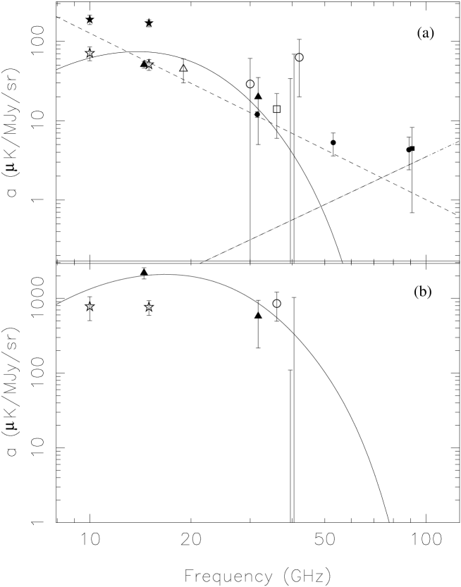
Figure 1: $a)$ Correlation slopes between CMB anisotropy data and the dust 100 $\mu$m template. Two standard deviation upper limits obtained for PyV from analysing all the fields and from analysing the SP94 overlap region only are both shown at $\sim 40$ GHz. $b)$ Correlations with the 12 $\mu$m template. Results are also shown for other experiments: Tenerife (open stars, de Oliveira-Costa et al. 2001; filled stars, Mukherjee et al. 2001), OVRO (filled triangles), 19GHz (open triangles), SP94 (open circles), Saskatoon (open square), Boomerang (filled rectangle), and DMR (filled circles). The solid curves are representative of a spinning dust spectrum, the dashed and the dot-dashed lines represent free-free and vibrational dust emission spectra, respectively.

References

- Benoît et al. (2003) Benoît, A., et al. 2003, A&A, 399, L25
- Coble et al. (1999) Coble, K., et al. 1999, ApJ, 519, L5
- Coble et al. (2003) Coble, K., Dodelson, S., Dragovan, M., Ganga, K., Knox, L., Kovac, J., Ratra, B., & Souradeep, T. 2003, ApJ, 584, 585
- de Oliveira-Costa et al. (1997) de Oliveira-Costa, A., Kogut, A., Devlin, M. J., Netterfield, C. B., Page, L. A., & Wollack, E. J. 1997, ApJ, 482, L17
- de Oliveira-Costa et al. (2000) de Oliveira-Costa, A., et al. 2000, ApJ, 542, L5
- de Oliveira-Costa et al. (2002) de Oliveira-Costa, A., et al. 2002, ApJ, 567, 363
- de Oliveira-Costa et al. (1999) de Oliveira-Costa, A., Tegmark, M., Gutierrez, C. M., Jones, A. W., Davies, R. D., Lasenby, A. N., Rebolo, R., & Watson, R. A. 1999, ApJ, 527, L9
- de Oliveira-Costa et al. (1998) de Oliveira-Costa, A., Tegmark, M., Page, L. A., & Boughn, S. P. 1998, ApJ, 509, L9
- Dragovan et al. (1994) Dragovan, M., Ruhl, J. E., Novak, G., Platt, S. R., Crone, B., Pernic, R., & Peterson, J. B. 1994 ApJ, 427, L67
- Draine & Lazarian (1998a) Draine, B. T., & Lazarian, A. 1998a, ApJ, 494, L19
- Draine & Lazarian (1998b) Draine, B. T., & Lazarian, A. 1998b, ApJ, 508, 157
- Draine & Lazarian (1999) Draine, B. T., & Lazarian, A. 1999, in ASP Conf. Ser. 181, Microwave Foregrounds, ed. A. de Oliveira-Costa & M. Tegmark (San Francisco: ASP), 133
- Finkbeiner et al. (2002) Finkbeiner, D. P., Schlegel, D. J., Frank, C., & Heiles, C. 2002, ApJ, 566, 898
- Fischler et al. (1985) Fischler, W., Ratra, B., & Susskind, L. 1985, Nucl. Phys. B, 259, 730
- Ganga et al. (1997) Ganga, K., Ratra, B., Gundersen, J. O., & Sugiyama, N. 1997, ApJ, 484, 7
- Ganga et al. (1998) Ganga, K., Ratra, B., Lim, M. A., Sugiyama, N., & Tanaka, S. T. 1998, ApJS, 114, 165
- Gaustad et al. (2001) Gaustad, J. E., McCullough, P. R., Rosing, W., & Van Buren, D. 2001, PASP, 113, 1326
- Gundersen et al. (1995) Gundersen, J. O., et al. 1995, ApJ, 443, L57
- Halverson et al. (2002) Halverson, N. W., et al. 2002, ApJ, 568, 38
- Hamilton, & Ganga (2001) Hamilton, J.-Ch., & Ganga K.M. 2001, A&A, 368, 760
- Haslam et al. (1981) Haslam, C. G. T., Klein, U., Salter, C. J., Stoffel, H., Wilson, W. E., Cleary, M. N., Cooke, D. J., & Thomasson, P. 1981, A&A, 100, 209
- Kogut (1999) Kogut, A. 1999, in ASP Conf. Ser. 181, Microwave Foregrounds, ed. A. de Oliveira-Costa & M. Tegmark (San Francisco: ASP), 91
- Kogut et al. (1996a) Kogut, A., Banday, A. J., Bennett, C. L., Górski, K. M., Hinshaw, G., & Reach, W. T. 1996a, ApJ, 460, 1
- Kogut et al. (1996b) Kogut, A., Banday, A. J., Bennett, C. L., Górski, K. M., Hinshaw, G., Smoot, G. F., & Wright, E. L. 1996b, ApJ, 464, L5
- Kuo et al. (2002) Kuo, C. L., et al. 2002, astro-ph/0212289
- Leitch et al. (1997) Leitch, E. M., Readhead, A. C. S., Pearson, T. J., & Myers, S. T. 1997, ApJ, 486, L23
- Lim et al. (1996) Lim, M. A., et al. 1996, ApJ, 469, L69
- Masi et al. (2001) Masi, S., et al. 2001, ApJ, 553, 93
- Mukherjee et al. (2002a) Mukherjee, P., Dennison, B., Ratra, B., Simonetti, J. H., Ganga, K., & Hamilton, J.-Ch. 2002a, ApJ, 579, 83
- Mukherjee et al. (2003) Mukherjee, P., Ganga, K., Ratra, B., Rocha, G., Souradeep, T., Sugiyama, N., & Górski, K. M. 2003, Intl. J. Mod. Phys., in press, astro-ph/0209567
- Mukherjee et al. (2001) Mukherjee, P., Jones, A. W., Kneissl, R., & Lasenby, A. N. 2001, MNRAS, 320, 224
- Mukherjee et al. (2002b) Mukherjee, P., Souradeep, T., Ratra, B., Sugiyama, N., & Górski, K. M. 2002b, astro-ph/0208216
- Page (2002) Page, L. 2002, astro-ph/0202145
- Park et al. (2002) Park, C.-G., Park, C., & Ratra, B. 2002, ApJ, 568, 9
- Park et al. (2001) Park, C.-G., Park, C., Ratra, B., & Tegmark, M. 2001, ApJ, 556, 582
- Peebles & Ratra (2003) Peebles, P. J. E., & Ratra, B. 2003, Rev. Mod. Phys, in press, astro-ph/0207347
- Platt et al. (1997) Platt, S. R., Kovac, J., Dragovan, M., Peterson, J. B., & Ruhl, J. E. 1997, ApJ, 475, L1
- Podariu et al. (2001) Podariu, S., Souradeep, T., Gott, J. R., Ratra, B., & Vogeley, M. S. 2001, ApJ, 559, 9
- Polenta et al. (2002) Polenta, G., et al. 2002, ApJ, 572, L27
- Ratra (1985) Ratra, B. 1985, Phys. Rev. D, 31, 1931
- Ratra et al. (1999a) Ratra, B., Ganga, K., Stompor, R., Sugiyama, N., de Bernardis, P., & Górski, K. M. 1999a, ApJ, 510, 11
- Ratra et al. (1999b) Ratra, B., Stompor, R., Ganga, K., Rocha, G., Sugiyama, N., & Górski, K. M. 1999b, ApJ, 517, 549
- Rocha et al. (1999) Rocha, G., Stompor, R., Ganga, K., Ratra, B., Platt, S. R., Sugiyama, N., & Górski, K. M. 1999, ApJ, 525, 1
- Ruhl et al. (2002) Ruhl, J. E., et al. 2002, astro-ph/0212229
- Ruhl et al. (1995) Ruhl, J. E., Dragovan, M., Platt, S. R., Kovac, J., & Novak, G. 1995, ApJ, 453, L1
- Santos et al. (2002) Santos, M. G., et al. 2002, Phys. Rev. Lett., 88, 241302
- Schlegel, Finkbeiner, & Davis (1998) Schlegel, D. J., Finkbeiner, D. P., & Davis, M. 1998, ApJ, 500, 525
- Shandarin et al. (2002) Shandarin, S. F., Feldman, H. A., Xu, Y., & Tegmark, M. 2002, ApJS, 141, 1
- Slosar et al. (2002) Slosar, A., et al. 2002, astro-ph/0212497
- Souradeep & Ratra (2001) Souradeep, T., & Ratra, B. 2001, ApJ, 560, 28
- Taylor et al. (2002) Taylor, A. C., et al. 2002, MNRAS, submitted, astro-ph/0205381
- Wright et al. (1994) Wright, A. E., Griffith, M. R., Burke, B. F., & Ekers, R. D. 1994, ApJS, 91, 111