Evolution of Cosmological Density Distribution Function from the Local Collapse Model

Abstract

We present a general framework to treat the evolution of one-point probability distribution function (PDF) for cosmic density $\delta$ and velocity-divergence fields $\theta$. In particular, we derive an evolution equation for the one-point PDFs and consider the stochastic nature associated with these quantities. Under the local approximation that the evolution of cosmic fluid fields can be characterized by the Lagrangian local dynamics with finite degrees of freedom, evolution equation for PDFs becomes a closed form and consistent formal solutions are constructed. Adopting this local approximation, we explicitly evaluate the one-point PDFs $P(\delta)$ and $P(\theta)$ from the spherical and the ellipsoidal collapse models as the representative Lagrangian local dynamics. In a Gaussian initial condition, while the local density PDF from the ellipsoidal model almost coincides with the that of the spherical model, differences between spherical and ellipsoidal collapse model are found in the velocity-divergence PDF. These behaviors have also been confirmed from the perturbative analysis of higher order moments. Importantly, the joint PDF of local density, $P(\delta,t;\delta^{\prime},t^{\prime})$, evaluated at the same Lagrangian position but at the different times $t$ and $t^{\prime}$ from the ellipsoidal collapse model exhibits a large amount of scatter. The mean relation between $\delta$ and $\delta^{\prime}$ does fail to match the one-to-one mapping obtained from spherical collapse model. Moreover, the joint PDF $P(\delta;\theta)$ from the ellipsoidal collapse model shows a similar stochastic feature, both of which are indeed consistent with the recent result from N-body simulations. Hence, the local approximation with ellipsoidal collapse model provides a simple but a more physical model than the spherical collapse model of cosmological PDFs, consistent with the leading-order results of exact perturbation theory.

1 INTRODUCTION

The large-scale structure of the universe is thought to be developed by the gravitational instability from the small Gaussian density fluctuations. In a universe dominated by dark matter, the evolution of mass distribution is entirely governed by gravitational dynamics. While luminous objects such as the galaxies and the clusters are subsequently formed by complicated processes including gas dynamics and radiative process, the dark matter distribution is the most fundamental product in the hierarchical clustering of the cosmic structure formation. In particular, the clustering feature of dark matter distribution is directly observed via weak gravitational lensing effect (Bartelmann & Schneider 2001 for review and references there in). Thus, the statistical study of the large-scale mass distribution provides a useful cosmological tool in probing the formation mechanism of dark matter halos, as well as the observed luminous distribution.

In principle, all the statistical information of dark matter distribution is characterized by the probability distribution functions (PDFs) for mass density fluctuation and velocity fields, $\delta$ and $v$. Among these, the one-point PDF for density field, $P(\delta)$, is one of the most fundamental statistical quantities and because of its simplicity, there has been numerous theoretical studies on its evolution from a Gaussian initial condition. From the analytical study of one-point PDFs, Kofman et al. (1994) first calculated the PDF using the Zel’dovich approximation. For a perturbative construction of one-point PDF, Bernardeau & Kofman (1995) and Juszkiewicz et al. (1995) introduced the Edgeworth expansion to derive the analytic formula for PDFs. On the other hand, based on the tree-level approximation, Bernardeau (1992b) constructed the PDF from the generating function of the vertex function. Interestingly, the vertex function in the tree-level approximation is obtained as an exact solution of the spherical collapse model. The effect of smoothing has been later incorporated into his calculation and the analytic PDF was compared with N-body simulations (Bernardeau, 1994b). Following these results, Fosalba & Gaztañaga (1998a) proposed to use the spherical collapse model for the prediction of higher-order moments beyond the tree-level approximation. The most remarkable point in their approximation is that the leading-order prediction exactly matches the one obtained from the rigorous perturbation theory and the correction for next-to-leading order is easily computed by solving the simple spherical collapse dynamics. Further, the spherical collapse approximation is recently extended to the prediction of one-point PDF (Scherrer & Gaztañaga 2001, see also Protogeros & Scherrer 1997). The approximation has been tested against N-body simulations and a good agreement was found even in a non-linear regime of the density perturbation.

On the other hand, from the numerical study, Kayo, Taruya & Suto (2001) recently showed that the log-normal PDF quantitatively approximates the one-point PDF $P(\delta)$ in the N-body simulations emerging from the Gaussian initial condition, irrespective of the shape of initial power spectra. The log-normal PDF has been long known as an empirical model characterizing the N-body simulations (e.g., Kofman et al., 1994; Bernardeau & Kofman, 1995; Taylor & Watts, 2000) or the observed galaxy distribution (e.g, Hamilton, 1985; Bouchet et al., 1993; Kofman et al., 1994). Recently, a good agreement with the log-normal model has been reported in the numerical study of weak lensing statistics (Taruya et al., 2002a), and an attempt to clarify the origin of the log-normal behavior has also made (Taruya et al., 2002b). Mathematically, the log-normal PDF is obtained from a one-to-one local mapping between the Gaussian and the non-linear density fields. Thus, the successful fit to the N-body simulation might be interpreted to imply that the evolution of local density can be well-approximated by the one-to-one local mapping. Indeed, the analytic PDF for the spherical collapse approximation can also be expressed as a one-to-one local mapping via the spherical collapse model.

The above naive picture has been critically examined by Kayo, Taruya & Suto (2001) evaluating the joint PDF $P(\delta_{1},t_{1};\,\delta_{2},t_{2})$, i.e., joint probability of the local density fields $\delta_{1}$ and $\delta_{2}$ at the same comoving position but at the different times $t_{1}$ and $t_{2}$. It has been found that a large amount of scatter in the relation between $\delta_{1}$ and $\delta_{2}$ shows up and their mean relation significantly deviates from the prediction from the one-to-one log-normal mapping. Although this might not be surprising, the good agreement between the log-normal and the simulated PDFs becomes more contrived and difficult to be explained in a straight forward manner.

Definitely, the failure of the one-to-one local mapping somehow reflects the non-locality of the gravitational dynamics. That is, the evolution of local density cannot be determined by the initial value of the local density only. Rather, the local density can be expressed as multi-variate functions of local density and other local quantities such as velocity, gradient of local density, velocity-divergence and so on. Furthermore, initial values of these local quantities are randomly distributed over the three-dimensional space. As a consequence, even if the dynamics is deterministic, the relation between the evolved and the initial local density inevitably becomes stochastic. In a sense, the situation is quite similar to the non-linear stochastic biasing of galaxies, i.e., the statistical uncertainty between galaxies and dark matter arising from the hidden variables (e.g., Dekel & Lahav, 1999; Taruya, Koyama & Soda, 1999; Taruya & Suto, 2000). Then, taking account of this stochastic nature, the crucial issue is to construct a simple but physically plausible model of one-point PDF, at least, consistent with the N-body simulations in a qualitative manner. Further, the influence of stochasticity on the evolution of local quantities should be investigated.

The purpose of this paper is to address these issues starting from a general theory of evolution of one-point PDF. In particular, we derive an evolution equation for the density and the velocity-divergence PDFs and consider how the stochastic nature of the local density field emerges. Due to the incompleteness of the equations, any theoretical approach using the evolution equations for PDFs generally becomes intractable. However, under the local approximation that the evolution of density field (or velocity-divergence) is entirely determined by the local dynamics with finite degrees of freedom, we explicitly show that the analytical solution for the evolution equations is consistently constructed. Based on this approximation, the one-point PDFs for the density and the velocity-divergence are computed from the ellipsoidal collapse model, as a natural extension of the one-to-one mapping of the spherical collapse approximation. Further, the stochastic nature arising from the multi-variate function of local quantities is explicitly shown evaluating the joint PDFs of the local density and/or the velocity-divergence. The influence of this effect is discussed in detail comparing with the spherical collapse approximation.

This paper is organized as follows. In section 2, we consider a general framework to treat the evolution of one-point PDFs and derive the evolution equations for the Eulerian and the Lagrangian PDFs (Sec.2.2 and 2.3). Then, adopting the local approximation, consistent solutions for these equations are obtained (Sec.2.4). Further, the stochastic nature of the evolution of PDFs is quantified evaluating joint PDFs (Sec.2.5). As an application of these general considerations, in section 3, we give an explicit evaluation of one-point PDFs adopting the spherical and the ellipsoidal collapse models as representative Lagrangian local dynamics. The qualitative features of the results are compared with the perturbative analysis presented in appendix B or the previous N-body study. Finally, section 4 is devoted to the conclusion and the discussion.

2 EVOLUTION EQUATION FOR PROBABILITY DISTRIBUTION FUNCTION

2.1 Preliminaries

Throughout the paper, we treat dark matter as a pressure-less and non-relativistic fluid. Assuming the homogeneous and isotropic background universe, the density field $\delta({\mbox{\boldmath$x$}},t)$, the peculiar velocity field ${\mbox{\boldmath$v$}}({\mbox{\boldmath$x$}},t)$ and the gravitational potential $\phi$ for the fluid follow the equation of continuity, the Euler equation and the Poisson equation as follows:

$$\frac{\partial\delta}{\partial t}+\frac{1}{a}\nabla\cdot\left\{(1+\delta){\mbox{\boldmath$v$}}\right\}=0,$$ (1)

$$\frac{\partial{\mbox{\boldmath$v$}}}{\partial t}+\frac{1}{a}({\mbox{\boldmath$v$}}\cdot\nabla){\mbox{\boldmath$v$}}+H{\mbox{\boldmath$v$}}=-\frac{1}{a}\nabla\phi,$$ (2)

$$\nabla^{2}\phi=4\pi G\,\rho_{\rm m}\,a^{2}\delta,$$ (3)

where $a$ is the scale factor of the universe, $H(\equiv\dot{a}/a)$ denotes the expansion rate and $\rho_{\rm m}$ is the background mass density.

While we are mainly interested in characterizing the large-scale structure on the basis of statistical properties of the density field $\delta({\mbox{\boldmath$x$}},t)$ and the velocity field ${\mbox{\boldmath$v$}}({\mbox{\boldmath$x$}},t)$ as described in section 1, the dynamical evolution of such quantities is not solely determined locally. Hence, we must introduce the other local quantities characterizing the non-local properties of gravitational evolution, e.g., the gradient of local density $\nabla\delta$, the velocity tensor $\partial_{i}v/\partial x_{j}$, and so on. Let us denote these variables by

$${\mbox{\boldmath${\cal F}$}}\equiv\left(\delta({\mbox{\boldmath$x$}},t),{\mbox{\boldmath$v$}}({\mbox{\boldmath$x$}},t),\nabla\delta({\mbox{\boldmath$x$}},t),\frac{\partial v_{i}}{\partial x_{j}}({\mbox{\boldmath$x$}},t),\cdots\right),$$ (4)

and define the joint PDF, $P({\mbox{\boldmath${\cal F}$}};t)$, which gives a probability density that the quantity ${\cal F}$ takes some values of $(\delta,{\mbox{\boldmath$v$}},\nabla\delta,\cdots)$ at the time $t$. In terms of this, the one-point PDF of the density fluctuations $P(\delta;t)$ is given as

$$P(\delta;t)=\int\prod_{{\cal F}_{i}\neq\delta}d{\cal F}_{i}\ P({\mbox{\boldmath${\cal F}$}};t),$$ (5)

and similarly the one-point PDF of the dimensionless velocity divergence, $P(\theta;t)$, is

$$P(\theta;t)=\int\prod_{{\cal F}_{i}\neq\theta}d{\cal F}_{i}\ P({\mbox{\boldmath${\cal F}$}};t),$$ (6)

where $\theta\equiv\nabla\cdot{\mbox{\boldmath$v$}}/(aH)$.

In general, a statistical characterization of the large-scale structure is coordinate-dependent. Physically, there are at least two meaningful coordinates, i.e., the Lagrangian and the Eulerian coordinates. While the Eulerian coordinate is fixed on a comoving frame, the Lagrangian coordinate is fixed on fluid particles and follows the motion of the fluid flow. Hence, as time goes on, high density regions in the Lagrangian space occupy larger volume than those in the Eulerian space. We thus consider both the Lagrangian PDF $P_{\scriptscriptstyle L}$ and the Eulerian PDF $P_{\scriptscriptstyle E}$, defined in the Lagrangian and the Eulerian coordinates, $q$ and $x$, respectively. The corresponding expectation values, $\langle\cdots\rangle_{\scriptscriptstyle L}$ and $\langle\cdots\rangle_{\scriptscriptstyle E}$ are also introduced.

In the following subsection, we first consider the Lagrangian PDF and derive the evolution equation. Then we derive the evolution equation for Eulerian PDF in section 2.3. The evolution equations derived here are not yet closed because of the unknown functions. In section 2.4 we discuss an approximate treatment using the local dynamics model, which enables us to obtain a closed form of evolution equation and to construct a consistent solution.

2.2 Lagrangian one-point PDF

To derive the evolution equation for the Lagrangian one-point PDF, we introduce an arbitrary function of local density, $g(\delta)$, and consider the evolution of its expectation value, $\langle g(\delta({\mbox{\boldmath$q$}},t))\rangle_{\scriptscriptstyle L}$ evaluated in a Lagrangian frame. The differentiation of this expectation value with respect to time becomes

$$\frac{\partial}{\partial t}\langle g(\delta({\mbox{\boldmath$q$}},t))\rangle_{\scriptscriptstyle L}=\frac{\partial}{\partial t}\int\prod_{i}d{\cal F}_{i}\ g(\delta)\,\,P_{\scriptscriptstyle L}({\mbox{\boldmath${\cal F}$}};t)=\int d\delta\ g(\delta)\,\,\frac{\partial}{\partial t}\,P_{\scriptscriptstyle L}(\delta;t),$$ (7)

since the explicit time dependence of the quantity $\langle g(\delta)\rangle_{\scriptscriptstyle L}$ only appears through the Lagrangian PDF. In the second equation, the integration is performed over the variable ${\cal F}$ except for the local density $\delta$. On the other hand, the function $g$ implicitly depends on time through the evolution of Lagrangian local density $\delta({\mbox{\boldmath$q$}},t)$. Denoting the Lagrangian time derivative by $d/dt\equiv\partial/\partial t+{\mbox{\boldmath$v$}}/a\cdot\nabla$, the expectation value of the quantity $dg/dt$ becomes

$$\left\langle\frac{d}{dt}\,\,g(\delta({\mbox{\boldmath$q$}},t))\right\rangle_{\scriptscriptstyle L}=\left\langle\frac{dg}{d\delta}\,\,\frac{d\delta}{dt}\right\rangle_{\scriptscriptstyle L}=\int\prod_{i}d{\cal F}_{i}\ \frac{dg(\delta)}{d\delta}\,\,\frac{d\delta}{dt}\,\,P_{\scriptscriptstyle L}({\mbox{\boldmath${\cal F}$}};t).$$ (8)

The right-hand-side of the above equation can be expressed by integrating by part as

$$\int\prod_{i}d{\cal F}_{i}\ \,\,\frac{dg(\delta)}{d\delta}\,\,\frac{d\delta}{dt}\,\,P_{\scriptscriptstyle L}({\mbox{\boldmath${\cal F}$}};t) = -\int\prod_{i}d{\cal F}_{i}\ g(\delta)\,\,\frac{\partial}{\partial\delta}\,\left\{\,\,\frac{d\delta}{dt}\,\,P_{\scriptscriptstyle L}({\mbox{\boldmath${\cal F}$}};t)\,\,\right\}$$ (9)

$$= -\int d\delta\ \,\,g(\delta)\,\,\frac{\partial}{\partial\delta}\,\left\{\,\,\left[\frac{d\delta}{dt}\right]_{\delta}P_{\scriptscriptstyle L}(\delta;t)\,\,\right\}.$$

Here, the quantity $[A]_{B}$ denotes the conditional mean of $A$ for a given value of $B$:

$$[A]_{B}\equiv\int\prod_{{\cal F}_{i}\neq B}d{\cal F}_{i}\ A\,\,P({\mbox{\boldmath${\cal F}$}}|B)$$ (10)

with the function $P({\mbox{\boldmath${\cal F}$}}|B)$ being the conditional PDF for a given $B$, i.e., $P({\mbox{\boldmath${\cal F}$}}|B)=P({\mbox{\boldmath${\cal F}$}})/P(B)$.

Now, recalling the fact that $g(\delta)$ is an arbitrary function of local density $\delta$, equation (7) must be equivalent to equation (8) in the Lagrange frame. The comparison between equation (7) and equation (9) then leads to the following evolution equation:

$$\frac{\partial}{\partial t}P_{\scriptscriptstyle L}(\delta;t)+\frac{\partial}{\partial\delta}\left(\left[\frac{d\delta}{dt}\right]_{\delta}P_{\scriptscriptstyle L}(\delta;t)\right)=0.$$ (11)

Similarly, one can derive the evolution equation for the Lagrangian PDF of the velocity divergence $P_{\scriptscriptstyle L}(\theta;t)$:

$$\frac{\partial}{\partial t}P_{\scriptscriptstyle L}(\theta;t)+\frac{\partial}{\partial\theta}\left(\left[\frac{d\theta}{dt}\right]_{\theta}P_{\scriptscriptstyle L}(\theta;t)\right)=0.$$ (12)

2.3 Eulerian one-point PDF

The evolution equation for the Eulerian one-point PDFs can also be derived by repeating the same procedure as above, but the resultant expressions are slightly different from those of the Lagrangian PDFs. The time derivative of the expectation value $\langle\,g(\delta)\,\rangle_{\scriptscriptstyle E}$ becomes

$$\frac{\partial}{\partial t}\langle g(\delta({\mbox{\boldmath$x$}},t))\rangle_{\scriptscriptstyle E}=\int d\delta\ g(\delta)\frac{\partial}{\partial t}P_{\scriptscriptstyle E}(\delta;t).$$ (13)

As for the expectation value of $\partial g/\partial t$, with a help of the Lagrangian time derivative, we obtain

$$\left\langle\frac{\partial}{\partial t}\,\,g(\delta({\mbox{\boldmath$x$}},t))\right\rangle_{\scriptscriptstyle E}=\left\langle\frac{dg}{d\delta}\frac{\partial\delta}{\partial t}({\mbox{\boldmath$x$}},t)\right\rangle_{\scriptscriptstyle E}=\left\langle\frac{dg}{d\delta}\frac{d\delta}{dt}({\mbox{\boldmath$x$}},t)\right\rangle_{\scriptscriptstyle E}-\left\langle\frac{dg}{d\delta}\frac{1}{a}{\mbox{\boldmath$v$}}\cdot\nabla\delta({\mbox{\boldmath$x$}},t)\right\rangle_{\scriptscriptstyle E}.$$ (14)

In the above expression, the first term in the second equation reduces to the same expression as in equation (9) just replacing the Lagrangian PDF with the Eulerian PDF. The second term in the second equation is further rewritten as

$$\left\langle\frac{dg}{d\delta}\,\,\frac{1}{a}\,\,{\mbox{\boldmath$v$}}\cdot\nabla\delta({\mbox{\boldmath$x$}},t)\right\rangle_{\scriptscriptstyle E} = \left\langle\frac{1}{a}\,\,{\mbox{\boldmath$v$}}\cdot\nabla g(\delta({\mbox{\boldmath$x$}},t))\right\rangle_{\scriptscriptstyle E}$$ (15)

$$= \frac{1}{a}\,\left\langle\nabla\cdot\{{\mbox{\boldmath$v$}}\,g(\delta({\mbox{\boldmath$x$}},t)\}\right\rangle_{\scriptscriptstyle E}\,\,-\,\,H\left\langle\theta\,g(\delta({\mbox{\boldmath$x$}},t))\right\rangle_{\scriptscriptstyle E}$$

$$= -H\,\int\prod_{i}\,d{\cal F}_{i}\,\,g(\delta)\,\theta\,P_{\scriptscriptstyle E}({\mbox{\boldmath${\cal F}$}};t),$$

where we have used the fact that the first term in the second line vanishes because of the isotropy. Then, using the definition of the conditional mean (10), equation (14) can be summarized as follows:

$$\left\langle\frac{\partial}{\partial t}g(\delta({\mbox{\boldmath$x$}},t))\right\rangle_{\scriptscriptstyle E} = \int d\delta\ g(\delta)\left\{-\frac{\partial}{\partial\delta}\left(\left[\frac{d\delta}{dt}(t)\right]_{\delta}P_{\scriptscriptstyle E}(\delta;t)\right)+H[\theta(t)]_{\delta}P_{\scriptscriptstyle E}(\delta;t)\right\}.$$ (16)

Hence, the relation $\langle\partial g/\partial t\rangle_{\scriptscriptstyle E}=\partial\langle g(\delta)\rangle_{\scriptscriptstyle E}/\partial t$, not the equation $\langle dg/dt\rangle_{\scriptscriptstyle E}=\partial\langle g(\delta)\rangle_{\scriptscriptstyle E}/\partial t$, leads to the evolution equation for the Eulerian one-point PDF $P(\delta,t)$. From equations (13) and (14), we obtain

$$\frac{\partial}{\partial t}P_{\scriptscriptstyle E}(\delta;t)+\frac{\partial}{\partial\delta}\left(\left[\frac{d\delta}{dt}(t)\right]_{\delta}P_{\scriptscriptstyle E}(\delta;t)\right)=H[\theta(t)]_{\delta}P_{\scriptscriptstyle E}(\delta;t).$$ (17)

Comparing equation (17) with equation (11), the only difference between the Eulerian and the Lagrangian PDF is the term $H[\theta]_{\delta}P_{\scriptscriptstyle E}$ in the right-hand-side of the above equation, which represents the change of the measure along the fluid trajectory in the Eulerian coordinate.

Finally, the evolution equation of the Eulerian one-point PDF $P_{\scriptscriptstyle E}(\theta;t)$ is also derived in a similar way:

$$\frac{\partial}{\partial t}P_{\scriptscriptstyle E}(\theta;t)+\frac{\partial}{\partial\theta}\left(\left[\frac{d\theta}{dt}(t)\right]_{\theta}P_{\scriptscriptstyle E}(\theta;t)\right)=H\theta P_{\scriptscriptstyle E}(\theta;t).$$ (18)

Note that the zero-mean of the velocity divergence $\langle\theta\rangle_{\scriptscriptstyle E}=0$ is always guaranteed from equation (18), which is easily shown by integrating the above equation over $\theta$ directly.

2.4 Local approximation

The evolution equations in the previous subsection are rather general and in deriving these we did not specify the dynamics of fluid evolution. In this sense, they are not closed until functional forms of the conditional means $\left[d\delta/dt\right]_{\delta}$, $\left[\theta\right]_{\delta}$ and $\left[d\theta/dt\right]_{\theta}$ are specified. In other words, these equations require the additional equations governing the evolution of the conditional means. However, an attempt to obtain the closed set of evolution equations suffers from serious mathematical difficulty, so-called closure problem, which is well-known in the subject of fluid mechanics and/or plasma physics (e.g., Chen et al., 1989; Goto & Kraichnan, 1993). Similar to the BBGKY hierarchy, if one derives the evolution equations for the conditional means, there appear new unknown conditional means. Thus, we must further repeat the derivation of evolution equation for the new quantities. Continuing this operation, one could finally obtain the infinite chain of the evolution equations, which is generally intractable.

Instead of the exact analysis tackling the difficult problem, we rather focus on an approximate treatment of the evolution of one-point PDFs, where the solutions for the evolution equations are consistently constructed. To implement this, we adopt the local approximation that the evolution of the local density $\delta$ and the velocity-divergence $\theta$ is described by the Lagrangian dynamics with finite degrees of freedom, whose initial conditions are characterized by the initial parameters, ${\mbox{\boldmath$p$}}=(p_{1},p_{2},\cdots p_{n})$, given at the same Lagrangian coordinate. As will be explicitly shown in the next section, for instance, if the spherical collapse model is adopted as Lagrangian local dynamics, the evolution of local density is characterized by the single variable, which can be set as the linearly extrapolated density fluctuation, $\delta_{l}$. If adopting the ellipsoidal collapse model, the dynamical degrees of freedom reduce to three, representing the principal axes of initial homogeneous ellipsoid, $\lambda_{1}$, $\lambda_{2}$ and $\lambda_{3}$. Thus, in this approximation, the density fluctuations can be expressed as $\delta=f({\mbox{\boldmath$p$}},t)$, and using this expression, the velocity-divergence is given by $\theta=-(df/dt)/H(1+f)$ from the equation of continuity (1). Within the local approximation, provided the initial distribution function $P_{\scriptscriptstyle I}({\mbox{\boldmath$p$}})$, the form of the conditional means can be completely specified and it can be expressed in terms of the functions $P_{\scriptscriptstyle I}({\mbox{\boldmath$p$}})$ and $f({\mbox{\boldmath$p$}},t)$.

Let us first consider the Lagrangian PDF. In this case, the formal expressions for the conditional means $\left[d\delta/dt\right]_{\delta}$ and $\left[d\theta/dt\right]_{\theta}$ are given by

$$\left[\frac{d\delta}{dt}\right]_{\delta}=\frac{1}{P_{\scriptscriptstyle L}(\delta;t)}\int\prod_{i}\,dp_{i}\,\,P_{\scriptscriptstyle I}({\mbox{\boldmath$p$}})\,\,\frac{df({\mbox{\boldmath$p$}},t)}{dt}\,\,\delta_{D}(\delta-f({\mbox{\boldmath$p$}},t)),$$ (19)

$$\left[\frac{d\theta}{dt}\right]_{\theta}=\frac{1}{P_{\scriptscriptstyle L}(\theta;t)}\int\prod_{i}dp_{i}\,\,P_{\scriptscriptstyle I}({\mbox{\boldmath$p$}})\,\,\frac{d}{dt}\left\{-\frac{1}{H(1+f)}\frac{df}{dt}\right\}\,\,\delta_{D}\left(\theta+\frac{1}{H(1+f)}\frac{df}{dt}\right).$$ (20)

With these expressions, the evolution equations (11) and (12) become a closed form and the consistent solutions can be constructed as follows:

$$P_{\scriptscriptstyle L}(\delta;t)= \int\prod_{i}dp_{i}\,\,P_{\scriptscriptstyle I}({\mbox{\boldmath$p$}})\,\,\delta_{D}(\delta-f({\mbox{\boldmath$p$}},t)),$$ (21)

$$P_{\scriptscriptstyle L}(\theta;t)= \int\prod_{i}dp_{i}\,\,P_{\scriptscriptstyle I}({\mbox{\boldmath$p$}})\,\,\delta_{D}\left(\theta+\frac{1}{H\{1+f({\mbox{\boldmath$p$}},t)\}}\frac{df({\mbox{\boldmath$p$}},t)}{dt}\right).$$ (22)

The proof that the above equations indeed satisfy the evolution equations (11) and (12) can be easily shown by differentiating equations (21) and (22) with respect to time. For the PDF of the local density, one has

$$\frac{\partial}{\partial t}P_{\scriptscriptstyle L}(\delta;t) = \int\prod_{i}dp_{i}\,\,P_{\scriptscriptstyle I}({\mbox{\boldmath$p$}})\,\frac{\partial}{\partial t}\,\delta_{D}(\delta-f({\mbox{\boldmath$p$}},t))$$

$$= \int\prod_{i}dp_{i}\,\,P_{\scriptscriptstyle I}({\mbox{\boldmath$p$}})\,\left(-\frac{df}{dt}\right)\,\frac{\partial}{\partial\delta}\,\delta_{D}(\delta-f({\mbox{\boldmath$p$}},t))$$

from the property of the Dirac’s delta function. In the above equation, the operator $\partial/\partial\delta$ in the last line can be factored out and one can use the expression of conditional mean (19). Then, the time derivative of the one-point PDF $P_{\scriptscriptstyle L}(\delta;t)$ is rewritten as

$$\frac{\partial}{\partial t}P_{\scriptscriptstyle L}(\delta;t)=-\frac{\partial}{\partial\delta}\,\left\{\,\left[\frac{d\delta}{dt}\right]_{\delta}\,P_{\scriptscriptstyle L}(\delta;t)\,\right\},$$ (23)

which coincides with the evolution equation (11). As for the velocity-divergence PDF $P_{\scriptscriptstyle L}(\theta;t)$, we consistently recover the evolution equation (12) with a help of equation (20):

$$\frac{\partial}{\partial t}P_{\scriptscriptstyle L}(\theta;t) = \int\prod_{i}dp_{i}\,\,P_{\scriptscriptstyle I}({\mbox{\boldmath$p$}})\,\,\frac{\partial}{\partial t}\,\,\delta_{D}\left(\theta+\frac{1}{H(1+f)}\frac{df}{dt}\right)$$ (24)

$$= \int\prod_{i}dp_{i}\,\,P_{\scriptscriptstyle I}({\mbox{\boldmath$p$}})\,\,\frac{d}{dt}\,\left\{\frac{1}{H(1+f)}\frac{df}{dt}\right\}\,\,\frac{\partial}{\partial\theta}\delta_{D}\left(\theta+\frac{1}{H(1+f)}\frac{df}{dt}\right)$$

$$= -\frac{\partial}{\partial\theta}\left(\left[\frac{d\theta}{dt}\right]_{\theta}P_{\scriptscriptstyle L}(\theta;t)\right).$$

The approximate solution of the Eulerian one-point PDFs are also obtained similarly, but the factor $1/(1+\delta)$ must be convolved with the Lagrangian PDF due to the presence of inertial term (r.h.s of eqs.[17][18]):

$$P_{\scriptscriptstyle E}(\delta;t)= \frac{1}{1+\delta}\int\prod_{i}dp_{i}\,\,P_{\scriptscriptstyle I}({\mbox{\boldmath$p$}})\,\,\delta_{D}(\delta-f({\mbox{\boldmath$p$}},t)),$$ (25)

$$P_{\scriptscriptstyle E}(\theta;t)= \int\prod_{i}dp_{i}\,\,\frac{P_{\scriptscriptstyle I}({\mbox{\boldmath$p$}})}{1+f}\,\,\delta_{D}\left(\theta+\frac{1}{H\{1+f({\mbox{\boldmath$p$}},t)\}}\,\frac{df}{dt}({\mbox{\boldmath$p$}},t)\right).$$ (26)

Note, however, that these PDFs do not satisfy the following conditions: normalization condition $\langle 1\rangle_{\scriptscriptstyle E}=1$ and zero means $\langle\delta\rangle_{\scriptscriptstyle E}=0$ and $\langle\theta\rangle_{\scriptscriptstyle E}=0$. This fact simply reflects that the conservation of Eulerian volume cannot be always guaranteed, in contrast to the conservation of Lagrangian volume ensured by the mass conservation. As pointed out by Fosalba & Gaztañaga (1998a) (see also Protogeros & Scherrer, 1997), we re-scale the relation between $\delta$ and $f({\mbox{\boldmath$p$}},t)$ as follows:

$$\delta=g({\mbox{\boldmath$p$}},t)\equiv N_{E}\,\{\,1+f({\mbox{\boldmath$p$}},t)\,\}\,-1~{}~{};\,\,\,N_{E}(t)\equiv\int\prod_{i}dp_{i}\,\,\frac{P_{\scriptscriptstyle I}({\mbox{\boldmath$p$}})}{1+f({\mbox{\boldmath$p$}},t)}.$$ (27)

Adopting this re-definition, the conditional means $\left[d\delta/dt\right]_{\delta}$ and $\left[d\theta/dt\right]_{\theta}$ become

$$\left[\frac{d\delta}{dt}\right]_{\delta} = \frac{1}{1+\delta}\,\,\frac{1}{P_{\scriptscriptstyle E}(\delta;t)}\int\prod_{i}dp_{i}\,\,P_{\scriptscriptstyle I}({\mbox{\boldmath$p$}})\,\,\frac{dg}{dt}({\mbox{\boldmath$p$}},t)\,\,\delta_{D}(\delta-g({\mbox{\boldmath$p$}},t)),$$ (28)

$$\left[\frac{d\theta}{dt}\right]_{\theta} = \frac{1}{P_{\scriptscriptstyle E}(\theta;t)}\int\prod_{i}dp_{i}\,\,\frac{P_{\scriptscriptstyle I}({\mbox{\boldmath$p$}})}{1+g}\,\,\frac{dh}{dt}({\mbox{\boldmath$p$}},t)\,\,\delta_{D}\left(\theta-h({\mbox{\boldmath$p$}},t)\right),$$ (29)

where we define

$$h({\mbox{\boldmath$p$}},t)\equiv-\frac{1}{H(1+g)}\frac{dg}{dt}.$$ (30)

Further, the conditional mean $[\theta]_{\delta}$ can be expressed as

$$\left[\theta\right]_{\delta}=-\frac{1}{H(1+\delta)}\left[\frac{d\delta}{dt}\right]_{\delta}$$ (31)

from the equation of continuity (1). Then, the solutions of equations (17) and (18) becomes

$$P_{\scriptscriptstyle E}(\delta;t)= \frac{1}{1+\delta}\int\prod_{i}dp_{i}\,\,P_{\scriptscriptstyle I}({\mbox{\boldmath$p$}})\,\,\delta_{D}(\delta-g({\mbox{\boldmath$p$}},t)),$$ (32)

$$P_{\scriptscriptstyle E}(\theta;t)= \int\prod_{i}dp_{i}\,\,\frac{P_{\scriptscriptstyle I}({\mbox{\boldmath$p$}})}{1+g}\,\,\delta_{D}\left(\theta-h({\mbox{\boldmath$p$}},t)\right).$$ (33)

One can easily show that equations (32) and (33) satisfy the evolution equations (17) and (18), with the correct normalization and the zero mean.

The above solutions for Eulerian PDF can be regarded as a generalization of the previous study based on the Zel’dovich approximation (Kofman et al., 1994) and/or the spherical collapse model (Scherrer & Gaztañaga 2001, see also Protogeros & Scherrer 1997). Note, however, that the general expression of velocity-divergence PDF $P_{\scriptscriptstyle E}(\theta;t)$ differs from the one obtained previously. While the factor $1/(1+\delta)$ is convolved in the integral in equation (33), the resultant expression by Kofman et al. (1994) obviously omitted this factor. In our prescription, the PDF $P_{\scriptscriptstyle E}(\theta;t)$ is constructed from the evolution equation, which basically relies on the equation of continuity. This means that, even for the velocity-divergence PDF, the factor $1/(1+\delta)$ is necessary to ensure the mass conservation. In fact, the expression (33) can also be obtained from the joint PDF $P_{\scriptscriptstyle E}(\delta,\theta;t)$ integrating over the local density $\delta$ (see eq.[36]). Although the velocity-divergence PDF in the previous study has been obtained in a rather phenomenological way, our present approach using the evolution equations might be helpful in constructing the consistent PDFs.

Nevertheless, even at this point, the solutions of evolution equations should be regarded as formal expressions. In order to evaluate the PDFs explicitly, we need to specify the Lagrangian local dynamics. In other words, the quantitative prediction for PDFs using the local approximation crucially depends on the choice of the local dynamics. We will see in the section 3 that the explicit evaluation of $P_{\scriptscriptstyle E}(\delta;t)$ and $P_{\scriptscriptstyle E}(\theta;t)$ adopting the spherical and the ellipsoidal collapse models shows several noticeable differences.

2.5 Joint PDF

So far, we have restricted our attention to the one-point PDF for the single local variable, $\delta$ or $\theta$. In our treatment of the local approximation, the expressions for PDFs are general forms irrespective of the Lagrangian local dynamics. However, it should be emphasized that if the local dynamics is characterized by more than the two initial parameters, qualitative behavior could be significantly changed from the local dynamics with single degree of freedom. The point is that the relation between initial parameters and the evolved result $\delta$ or $\theta$ cannot be described by a one-to-one mapping. Accordingly, the relation between $\delta$ and $\theta$ becomes no longer deterministic. Moreover, the failure of deterministic property also appears in the time evolution of such local variables. It is therefore important to discuss the stochastic nature of $\delta$ and $\theta$ arising from the dynamical evolution. To characterize this, we consider the joint PDF. Within the local approximation, one can construct a consistent solution of Eulerian joint PDF between $\delta$ and $\theta$ evaluated at the same time, $P_{\scriptscriptstyle E}(\delta,\theta;t)$. Further, the Lagrangian joint PDF for the density field evaluated at the same Lagrangian position but at the different times, $P_{\scriptscriptstyle L}(\delta,t;\delta^{\prime},t^{\prime})$ can also be obtained.

The evolution equation of $P_{\scriptscriptstyle E}(\delta,\theta;t)$ can be derived through the expectation value of an arbitrary function $g(\delta,\theta)$. Repeating the same procedure as described in section 2.3, we obtain

$${\displaystyle\frac{\partial}{\partial t}\langle g(\delta({\mbox{\boldmath$x$}},t),\theta({\mbox{\boldmath$x$}},t))\rangle_{\scriptscriptstyle E}} =\int d\delta d\theta\ g(\delta,\theta)\frac{\partial}{\partial t}P_{\scriptscriptstyle E}(\delta,\theta;t),$$

$${\displaystyle\left\langle\frac{\partial}{\partial t}g(\delta({\mbox{\boldmath$x$}},t),\,\theta({\mbox{\boldmath$x$}},t))\right\rangle_{\scriptscriptstyle E}} =\left\langle\frac{\partial g}{\partial\delta}\frac{d\delta}{dt}+\frac{\partial g}{\partial\theta}\frac{d\theta}{dt}+H\theta g(\delta,\theta)\right\rangle_{\scriptscriptstyle E}$$

$$=\int d\delta d\theta\ g(\delta,\theta)\left\{-\frac{\partial}{\partial\delta}\left(\left[\frac{d\delta}{dt}\right]_{\delta,\theta}P_{\scriptscriptstyle E}(\delta,\theta;t)\right)\right.$$

$$~{}~{}~{}~{}~{}~{}~{}~{}~{}~{}~{}~{}~{}\left.-\frac{\partial}{\partial\theta}\left(\left[\frac{d\theta}{dt}\right]_{\delta,\theta}P_{\scriptscriptstyle E}(\delta,\theta;t)\right)+H\theta P_{\scriptscriptstyle E}(\delta,\theta;t)\right\}.$$

Then, these two equations lead to the evolution equation for $P_{\scriptscriptstyle E}(\delta,\theta;t)$:

$$\frac{\partial}{\partial t}P_{\scriptscriptstyle E}(\delta,\theta;t)-H\theta\frac{\partial}{\partial\delta}\left\{(1+\delta)P_{\scriptscriptstyle E}(\delta,\theta;t)\right\}+\frac{\partial}{\partial\theta}\left(\left[\frac{d\theta}{dt}\right]_{\delta,\theta}P_{\scriptscriptstyle E}(\delta,\theta;t)\right)=H\theta P_{\scriptscriptstyle E}(\delta,\theta;t),$$ (34)

where we used the relation $[d\delta/dt]_{\delta,\theta}=-H\theta(1+\delta)$.

The construction of the consistent solution in the local approximation is almost parallel to the case of the Eulerian one-point PDF in section 2.4. The formal expression of the conditional mean $[d\theta/dt]_{\delta,\theta}$ is

$$\left[\frac{d\theta}{dt}\right]_{\delta,\theta}=\frac{1}{P_{\scriptscriptstyle E}(\delta,\theta;t)}\frac{1}{1+\delta}\int\prod dp_{i}\ \,\,P_{\scriptscriptstyle I}({\mbox{\boldmath$p$}})\,\,\frac{dh}{dt}\,\,\delta_{D}(\delta-g({\mbox{\boldmath$p$}},t))\delta_{D}(\theta-h({\mbox{\boldmath$p$}},t)),$$ (35)

and the corresponding solution of equation (34) becomes

$$P_{\scriptscriptstyle E}(\delta,\theta;t)=\frac{1}{1+\delta}\int\prod_{i}dp_{i}\,\,P_{\scriptscriptstyle I}({\mbox{\boldmath$p$}})\,\,\delta_{D}(\delta-g({\mbox{\boldmath$p$}},t))\delta_{D}(\theta-h({\mbox{\boldmath$p$}},t)).$$ (36)

Note again that the above solution exactly recovers the one-point PDFs $P_{\scriptscriptstyle E}(\delta;t)$ and $P_{\scriptscriptstyle E}(\theta;t)$ integrating equation (36) over $\theta$ and $\delta$, respectively (see eqs.[32][33]).

The evolution equation for Lagrangian joint PDF is also obtained by the time derivative of the expectation value of the arbitrary function, $g(\delta({\mbox{\boldmath$q$}},t),\delta({\mbox{\boldmath$q$}},t^{\prime}))$ as described in section 2.2:

$${\displaystyle\frac{d}{dt}\left\langle g(\delta({\mbox{\boldmath$q$}},t),\delta({\mbox{\boldmath$q$}},t^{\prime}))\right\rangle} =\int d\delta d\delta^{\prime}g(\delta,\delta^{\prime})\frac{\partial}{\partial t}P_{\scriptscriptstyle L}(\delta,t;\delta^{\prime},t^{\prime}),$$

$${\displaystyle\left\langle\frac{d}{dt}g(\delta({\mbox{\boldmath$q$}},t),\delta({\mbox{\boldmath$q$}},t^{\prime}))\right\rangle} =\left\langle\frac{\partial}{\partial\delta({\mbox{\boldmath$q$}},t)}g(\delta({\mbox{\boldmath$q$}},t),\delta({\mbox{\boldmath$q$}},t^{\prime}))\frac{d\delta({\mbox{\boldmath$q$}},t)}{dt}\right\rangle$$

$$=-\int d\delta d\delta^{\prime}g(\delta,\delta^{\prime})\frac{\partial}{\partial\delta}\left(\left[\frac{d\delta}{dt}\right]_{\delta,\delta^{\prime}}P_{\scriptscriptstyle L}(\delta,t;\delta^{\prime},t^{\prime})\right).$$

The evolution equation of Lagrangian joint PDF is

$$\frac{\partial}{\partial t}P_{\scriptscriptstyle L}(\delta,t;\delta^{\prime},t^{\prime})+\frac{\partial}{\partial\delta}\left(\left[\frac{d\delta}{dt}\right]_{\delta,\delta^{\prime}}P_{\scriptscriptstyle L}(\delta,t;\delta^{\prime},t^{\prime})\right)=0.$$ (37)

The conditional mean in the local approximation is expressed as

$$\left[\frac{d\delta}{dt}\right]_{\delta,\delta^{\prime}} = \frac{1}{P_{\scriptscriptstyle L}(\delta,t;\delta^{\prime},t^{\prime})}\int\prod_{i}dp_{i}\,\,P_{\scriptscriptstyle I}({\mbox{\boldmath$p$}})\,\,\frac{df({\mbox{\boldmath$p$}},t)}{dt}\,\,\delta_{D}(\delta-f({\mbox{\boldmath$p$}},t))\,\delta_{D}(\delta^{\prime}-f({\mbox{\boldmath$p$}},t^{\prime})).$$

Recalling that the joint PDF satisfying the evolution equation (37) should be invariant under the transformation, $(\delta,t)\leftrightarrow(\delta^{\prime},t^{\prime})$, the solution consistent with the boundary condition $P_{\scriptscriptstyle L}(\delta,t^{\prime};\delta^{\prime},t^{\prime})=P_{\scriptscriptstyle L}(\delta;t^{\prime})\delta_{D}(\delta-\delta^{\prime})$ becomes

$$P_{\scriptscriptstyle L}(\delta,t;\delta^{\prime},t^{\prime}) = \int\prod_{i}dp_{i}\,\,P_{\scriptscriptstyle I}({\mbox{\boldmath$p$}})\,\,\delta_{D}(\delta-f({\mbox{\boldmath$p$}},t))\,\delta_{D}(\delta^{\prime}-f({\mbox{\boldmath$p$}},t^{\prime})).$$ (38)

Notice that if the local Lagrangian dynamics is described by a single parameter, the integral over the initial parameter $p_{1}$ in equation (38) can be formally performed. The resultant expression includes Dirac’s delta function, leading to the one-to-one mapping between $\delta$ and $\delta^{\prime}$. On the other hand, in cases with the multivariate initial parameters, one cannot generally perform the above integral and the Dirac’s delta function is not factored out, leading to the stochastic nature of local density fields.

One might further consider the evolution of Eulerian joint PDF $P_{\scriptscriptstyle E}(\delta,t;\delta^{\prime},t^{\prime})$, which has been indeed shown in N-body simulations by Kayo et al. (2001). The derivation of evolution equation itself is an easy task, but, the formal solution in the local approximation suffers from difficulties due to the presence of advective term, which might be related to an important effect on the non-local nature of fluid flows. Since even the Lagrangian joint PDF shows several important features, one can expect that the qualitatively similar behavior to the N-body results can be seen from the Lagrangian joint PDF. Hence, we will postpone to analyze the Eulerian joint PDF $P_{\scriptscriptstyle E}(\delta,t;\delta^{\prime},t^{\prime})$ and instead focus on the Lagrangian joint PDF $P_{\scriptscriptstyle L}(\delta,t^{\prime};\delta^{\prime},t^{\prime})$.

3 DEMONSTRATION AND RESULTS

Now we are in a position to give an explicit evaluation of the one-point PDF based on the local approximation discussed in the previous section. For an illustrative purpose, we adopt the spherical and the ellipsoidal collapse models as simple and intuitive Lagrangian local dynamics. After briefly describing the basic equations of these models in section 3.1, we compute the Eulerian one-point PDFs $P_{\scriptscriptstyle E}(\delta)$ and $P_{\scriptscriptstyle E}(\theta)$ and discuss the qualitative differences arising from the choice of Lagrangian local dynamics in section 3.2. In particular the stochasticity in the multi-variate function of local density or velocity-divergence is examined in detail by evaluating the joint PDFs, $P_{\scriptscriptstyle L}(\delta,t;\delta^{\prime},t^{\prime})$ and $P_{\scriptscriptstyle E}(\delta;\theta)$ from the ellipsoidal collapse model.

3.1 Models for Lagrangian local dynamics

First consider the simplest case of the Lagrangian local dynamics, in which the evolution of local quantities is determined by the mass inside a sphere of radius $R$ collapsing via self-gravity:

$$\frac{d^{2}R}{dt^{2}}=-\frac{GM}{R^{2}}~{}~{}~{}~{}~{};~{}~{}M=\frac{4\pi}{3}\,\,\overline{\rho}\,\,R^{3}=\mbox{const},$$ (39)

where $M$ is the mass inside the radius and $\overline{\rho}$ represents the local density. This spherical collapse model can be re-expressed as the evolution equation for density fluctuations $\delta$, given by $\delta=\overline{\rho}/\rho_{\rm m}-1=(a/R)^{3}-1$ as follows:

$$\frac{d^{2}\delta}{dt^{2}}+2H\frac{d\delta}{dt}-\frac{4}{3}\frac{1}{1+\delta}\left(\frac{d\delta}{dt}\right)^{2}=\frac{3}{2}H^{2}\Omega_{\rm m}(1+\delta)\delta,$$ (40)

with the quantity $\Omega_{\rm m}$ being the density parameter, $\Omega_{\rm m}\equiv 8\pi G\,\rho_{\rm m}/(3H^{2})$. As Fosalba & Gaztañaga (1998a) stated, this equation is regarded as a shear-less and irrotational approximation of fluid equations, since one can derive the following equation from equations (1) to (3) :

$$\frac{d^{2}\delta}{dt^{2}}+2H\frac{d\delta}{dt}-\frac{4}{3}\frac{1}{1+\delta}\left(\frac{d\delta}{dt}\right)^{2}=H^{2}(1+\delta)\left(\frac{3}{2}\Omega_{\rm m}\delta+\sigma^{ij}\sigma_{ij}-\omega^{ij}\omega_{ij}\right),$$ (41)

with a help of the Lagrangian time derivative. Here the quantities $\sigma_{ij}$ and $\omega_{ij}$ respectively denote the shear and the rotation given by

$$\sigma_{ij} = \frac{1}{2aH}\left(\frac{\partial v_{i}}{\partial x_{j}}+\frac{\partial v_{j}}{\partial x_{i}}\right)-\frac{1}{3}\,\,\theta\,\,\delta_{ij},$$ (42)

$$\omega_{ij} = \frac{1}{2aH}\left(\frac{\partial v_{i}}{\partial x_{j}}-\frac{\partial v_{j}}{\partial x_{i}}\right).$$ (43)

In the spherical collapse approximation (40), the density fluctuations $\delta$ depend only on a single initial parameter $\delta_{l}$, i.e., the linear fluctuation at an initial time, if the decaying mode of the linear perturbation is neglected. Note that the spatial distribution of the initial density field is randomly given and thereby the parameter $\delta_{l}$ is regarded as a random variable. We assume that the initial parameter $\delta_{l}$ obeys a Gaussian distribution:

$$P_{\scriptscriptstyle I}(\delta_{l})=\frac{1}{\sqrt{2\pi}\,\,\sigma_{l}}\,\,e^{-(\delta_{l}/\sigma_{l})^{2}/2},$$ (44)

where the variable $\sigma_{l}$ means the rms fluctuation of the linear density field $\delta_{l}$, i.e., $\sigma_{l}^{2}=\langle\delta_{l}^{2}\rangle$.

The ellipsoidal collapse approximation which is another Lagrangian local dynamics, describes the evolution of the uniform density ellipsoid. In contrast to the spherical collapse model, the evolution of $\delta$ is governed by the dynamics of the half length of principal axes $\alpha_{i}$ $(i=1,2,3)$ characterizing the density ellipsoid. According to Bond & Myers (1996), we have

$$\frac{d^{2}}{dt^{2}}\alpha_{i}=-4\pi G\,\rho_{m}\,\alpha_{i}\left(\frac{1+\delta}{3}+\frac{b_{i}}{2}\delta+\lambda_{{\rm ext},i}\right),$$ (45)

$$b_{i}=\alpha_{1}\alpha_{2}\alpha_{3}\int_{0}^{\infty}\frac{d\tau}{(\alpha_{i}^{2}+\tau)\prod_{j}(\alpha_{j}^{2}+\tau)^{1/2}}-\frac{2}{3},$$ (46)

and the relation between $\delta$ and $\alpha_{i}$ becomes

$$\delta=\frac{a^{3}}{\alpha_{1}\alpha_{2}\alpha_{3}}-1.$$ (47)

Here, the variable $\lambda_{{\rm ext},i}$ quantifies the external tidal effect, which is required for the consistency with the Zel’dovich approximation in a linear regime (Bond & Myers, 1996):

$$\lambda_{{\rm ext},i}=\cases{\displaystyle D(t)\,\left(\lambda_{i}-\frac{\lambda_{1}+\lambda_{2}+\lambda_{3}}{3}\right)&; linear external tide ,\cr\frac{5}{4}\,b_{i}&; nonlinear external tide ,}$$ (48)

where $D(t)$ is the linear growth rate. The variables $\lambda_{i}$ represent the initial parameters of principal axes, and in terms of these, the initial conditions reduce to

$$\alpha_{i}(t_{0}) = a(t_{0})\{1-D(t_{0})\lambda_{i}\},$$ (49)

$$\frac{d}{dt}\alpha_{i}(t_{0}) = \dot{a}(t_{0})\{1-D(t_{0})\lambda_{i}\}-a(t_{0})\dot{D}(t_{0})\lambda_{i}.$$ (50)

In contrast to the spherical collapse model, one can regard this model as an approximation of the fluid equations taking account of the influence of shear but neglecting the rotation:

$$\frac{d^{2}\delta}{dt^{2}}+2H\frac{d\delta}{dt}-\frac{4}{3}\frac{1}{1+\delta}\left(\frac{d\delta}{dt}\right)^{2}=H^{2}(1+\delta)\left(\frac{3}{2}\Omega_{\rm m}\delta+\sigma^{ij}\sigma_{ij}\right);$$ (51)

$$~{}~{}~{}~{}~{}~{}~{}~{}~{}~{}~{}~{}~{}~{}~{}\sigma_{ij}=\frac{1}{3H}\left(3\frac{\dot{\alpha_{i}}}{\alpha_{i}}-\frac{\dot{\alpha_{1}}}{\alpha_{1}}-\frac{\dot{\alpha_{2}}}{\alpha_{2}}-\frac{\dot{\alpha_{3}}}{\alpha_{3}}\right)\,\delta_{ij}.$$

Note that similar to the spherical collapse approximation, the three initial parameters $\lambda_{i}$ are regarded as the random variables. When the initial condition of density field is assumed to be a Gaussian random distribution, the expression for the initial parameter distribution $P_{\scriptscriptstyle I}(\lambda_{i})$ is analytically obtained as follows (e.g., Doroshkevich, 1970; Bardeen et al., 1986):

$$P_{\scriptscriptstyle I}(\lambda_{i})=\frac{3375}{8\sqrt{5}\pi\sigma_{l}^{6}}\exp\left(-3\frac{I_{1}^{2}}{\sigma_{l}^{2}}+15\frac{I_{2}}{2\sigma_{l}^{2}}\right)(\lambda_{1}-\lambda_{2})(\lambda_{2}-\lambda_{3})(\lambda_{1}-\lambda_{3}),$$ (52)

where the quantities $I_{1}$ and $I_{2}$ denote $I_{1}\equiv\lambda_{1}+\lambda_{2}+\lambda_{3}$ and $I_{2}\equiv\lambda_{1}\lambda_{2}+\lambda_{2}\lambda_{3}+\lambda_{3}\lambda_{1}$, respectively.

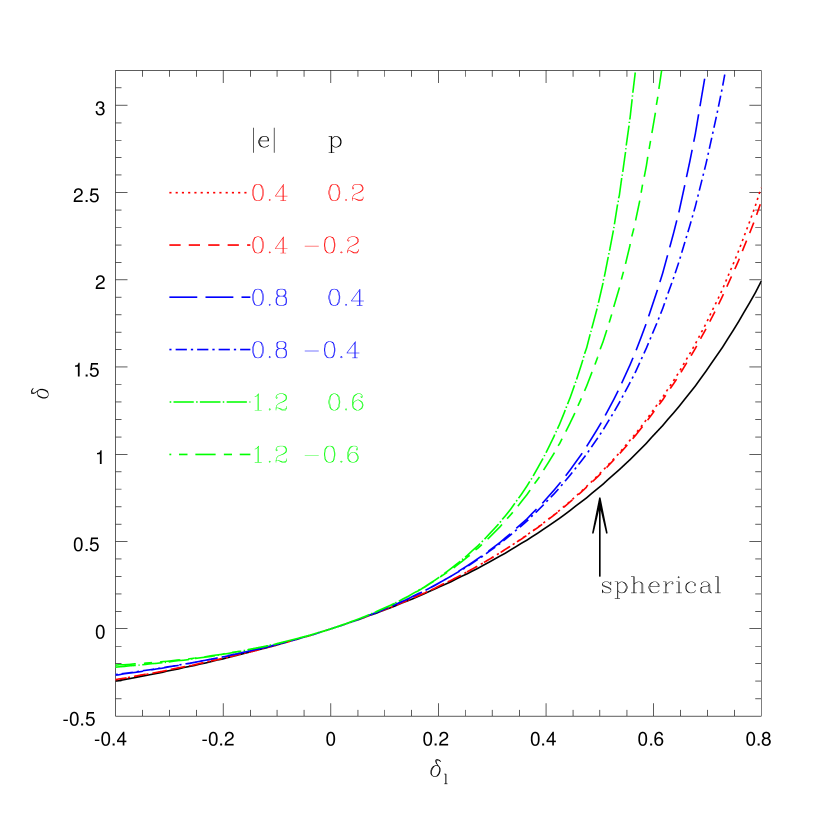
Figure 1: Evolution of local density from the ellipsoidal collapse model for various initial parameters, $(e,p)$, where $e$ is ellipticity and $p$ is prolateness, given by $e=(\lambda_{1}-\lambda_{3})/(2\delta_{l})$ and $p=(\lambda_{1}+\lambda_{3}-2\lambda_{2})/(2\delta_{l})$, respectively. The evolved results are then plotted as a function of linearly extrapolated density, $\delta_{l}=\lambda_{1}+\lambda_{2}+\lambda_{3}$. For comparison, we also plot the one-to-one local mapping from the spherical collapse model (solid).

Based on these Lagrangian local models, we numerically calculate the PDFs assuming the Einstein-de Sitter universe ($\Omega_{\rm m}=1$, $\Omega_{\Lambda}=0$), in which the linear growth rate $D$ is simply proportional to the scale factor $a$. For a better understanding of the later analysis, in Figure 1, we plot the evolution of local density $\delta$ from the ellipsoidal collapse model for some initial conditions $(e,p)$ given by $e=(\lambda_{1}-\lambda_{3})/(2\delta_{l})$ and $p=(\lambda_{1}+\lambda_{3}-2\lambda_{2})/(2\delta_{l})$. The results are then depicted as a function of linearly extrapolated density $\delta_{l}=\lambda_{1}+\lambda_{2}+\lambda_{3}$ and are compared with the one from the one-to-one mapping of spherical collapse model (solid). Figure 1 shows that the local density of the ellipsoidal collapse model generally takes a larger value than that of the spherical collapse model. Further, the variety of evolved density for fixed $\delta_{l}$ suggests that a large amount of scatter will appear in the joint PDF $P_{\scriptscriptstyle L}(\delta,t;\delta^{\prime},t^{\prime})$ and the resultant one-point PDFs $P_{\scriptscriptstyle E}(\delta)$ and $P_{\scriptscriptstyle E}(\theta)$ cannot, in general, coincide with those obtained from the spherical collapse model.

3.2 Results

In computing the PDFs from the above local collapse models, one may practically encounter the case when the local density infinitely diverges at finite elapsed time for some regions in the initial parameter space, which has not been treated in previous section. To avoid the unphysical divergences, we must restrict the integral in the PDFs to the initial parameter space $V(t)$, in which the local density $\delta$ does not diverge. Indeed, this modification slightly affects the normalization condition for both the Lagrangian and the Eulerian PDFs, i.e., $\langle\,1\,\rangle_{\scriptscriptstyle L,E}\neq 1$. Although this does not alter any qualitative features of PDFs, we consider some modifications to keep the correct normalization and adopting this procedure in appendix A, and the results for one-point and joint PDFs are presented below. Note, however, that the perturbation calculation discussed in 3.2.1 is free from the serious divergences and within the perturbative treatment, one can rigorously develop the local approximation for PDFs.

3.2.1 One-point PDFs

Let us show the results of the one-point PDF. Figure 2 plots the one-point Eulerian PDFs of the local density (top) and the velocity-divergence (bottom) evaluated at various linear fluctuation values $\sigma_{l}$. In both panels, the thick lines represent the results obtained from the ellipsoidal collapse model with linear external tide, while the thin lines denote the PDFs from the spherical collapse models. In computing the PDFs, the Lagrangian local dynamics are numerically solved with the various initial conditions $p$ in the initial parameter space $V$. Then, weighting by the PDF of the initial parameter $P_{\scriptscriptstyle I}({\mbox{\boldmath$p$}})$, the PDFs are constructed by binning the evolved results of the density $\delta$ and the velocity-divergence $\theta$, together with appropriate convolution factors (see Appendix A).

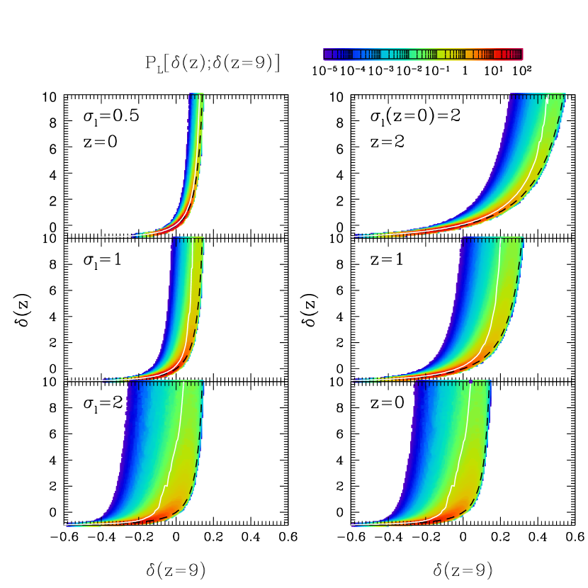
Figure 4: Contour plot of Lagrangian joint PDF $P_{\scriptscriptstyle L}(\delta(z),\delta(z=9))$ obtained from the ellipsoidal collapse model with linear external tide. The left panel shows the results fixing the redshift to $z=0$, while the right panel represents the evolution of joint PDF fixing the linear variance to $\sigma_{l}=2$. In each panel, solid lines indicate the conditional mean $[\delta(z)]_{\delta(z=9)}$ computed from joint PDF. For comparison, the one-to-one local mapping obtained from the spherical collapse model are also plotted in short-dashed lines. Left: $\sigma_{l}=0.5$(top), $\sigma_{l}=1$(middle) and $\sigma_{l}=2$(bottom). Right: $z=2$(top), $z=1$(middle) and $z=0$(bottom).

As expected, the overall behaviors of both PDFs in Figure 2 are qualitatively similar, irrespective of the Lagrangian local models. As increasing the linear fluctuation value $\sigma_{l}$, while the density PDF $P_{\scriptscriptstyle E}(\delta)$ extends over the high-density region $\delta\gg 1$, the velocity-divergence PDF $P_{\scriptscriptstyle E}(\theta)$ is negatively skewed and it extends over the negative region $\theta\ll-1$. In looking at the differences in each local model, we readily observe several remarkable features. First, the density PDFs computed from both the spherical and the ellipsoidal collapse models almost agree with each other. At first glance, this seems to contradict with a naive expectation from the local dynamics in Figure 1. However, one might rather suspect that the agreement in density PDFs is accidental, due to the distribution of initial parameters $P_{\scriptscriptstyle I}(\lambda_{i})$, which is, at least, consistent with a naive picture that joint PDF $P_{\scriptscriptstyle L}(\delta,t;\delta^{\prime},t^{\prime})$ from the ellipsoidal collapse model exhibits a large mount scatter and the mean relation between $\delta$ and $\delta^{\prime}$ significantly deviates from one-to-one mapping of spherical collapse model (see Sec.3.2.2 and Fig.4). On the other hand, the velocity-divergence PDFs from the ellipsoidal collapse model exhibit longer non-Gaussian tails, compared with those obtained from the spherical collapse model. The deviation between both models in PDF $P_{\scriptscriptstyle E}(\theta)$ becomes significant as increasing the value $\sigma_{l}$. Interestingly, in the non-linear regime $\sigma_{l}\geq 1$, tails of PDF $P_{\scriptscriptstyle E}(\theta)$ from the spherical collapse model show the opposite tendency, i.e., the amplitude decreases as increasing $\sigma_{l}$.

In order to characterize the qualitative behaviors more explicitly, we perturbatively solve the evolution equations for both the spherical and the ellipsoidal collapse models. The differences are then quantified evaluating the higher order moments of one-point statistics for the local density and velocity-divergence. In appendix B, based on the formal solution of PDFs in section 2.4, perturbative calculations of local collapse models are briefly summarized and the solutions up to the fifth order are presented. The resultant expressions for the higher order moments of density and velocity-divergence are obtained as a series expansion of linear variance $\sigma_{l}^{2}$, up to the two-loop order for the variance and the one-loop order for the skewness and the kurtosis:

$$\sigma^{2} \equiv \langle\delta^{2}\rangle_{\scriptscriptstyle E}=\sigma_{l}^{2}+s_{2,4}\,\,\sigma_{l}^{4}+s_{2,6}\,\,\sigma_{l}^{6}+\cdots,$$ (53)

$$S_{3} \equiv \frac{\langle\delta^{3}\rangle_{\scriptscriptstyle E}}{\sigma^{4}}=S_{3,0}+S_{3,2}\,\,\sigma_{l}^{2}+\cdots,$$ (54)

$$S_{4} \equiv \frac{\langle\delta^{4}\rangle_{\scriptscriptstyle E}-3\sigma^{4}}{\sigma^{6}}=S_{4,0}+S_{4,2}\,\,\sigma_{l}^{2}+\cdots$$ (55)

for the local density and

$$\sigma_{\theta}^{2} \equiv \langle\theta^{2}\rangle_{\scriptscriptstyle E}=\sigma_{l}^{2}+s_{2,4}^{\theta}\,\,\sigma_{l}^{4}+s_{2,6}^{\theta}\,\,\sigma_{l}^{6}+\cdots,$$ (56)

$$T_{3} \equiv \frac{\langle\theta^{3}\rangle_{\scriptscriptstyle E}}{\sigma_{\theta}^{4}}=T_{3,0}+T_{3,2}\,\,\sigma_{l}^{2}+\cdots,$$ (57)

$$T_{4} \equiv \frac{\langle\theta^{4}\rangle_{\scriptscriptstyle E}-3\sigma_{\theta}^{4}}{\sigma_{\theta}^{6}}=T_{4,0}+T_{4,2}\,\,\sigma_{l}^{2}+\cdots$$ (58)

for the velocity-divergence. Then, all the coefficients in the above expansions yield the rigorous fractional number and Table 1 displays a summary of the results. The calculation in spherical collapse model essentially reproduces the non-smoothing results obtained by Fosalba & Gaztañaga (1998a, b). Note, however, that the discrepancy has appeared in the higher order correction of velocity-divergence (c.f., eq.[12] with $\gamma=0$ of Fosalba & Gaztañaga, 1998b). Perhaps, in computing the velocity-divergence moments, Fosalba & Gaztañaga (1998b) incorrectly used the cumulant expansion formula for $\delta$ listed in Fosalba & Gaztañaga (1998a). Further, we suspect that they erroneously replaced the convolution factor $1/(1+\delta)$ in Eulerian expectation value with $1/(1+\theta)$. On the other hand, in our calculation, moments $\langle\theta^{n}\rangle_{\scriptscriptstyle E}$ are rigorously computed according to the definition (B6), with a help of the velocity-divergence PDF (33) with equation (30). Hence, the present calculation is at least consistent with the local approximation in section 2.4 and we believe that no serious error has appeared in present result.

Apart from this discrepancy, one finds that the leading-order (tree-level) calculation of skewness $S_{3,0}$ and kurtosis $S_{4,0}$ in both models exactly coincides with each other. While the differences in the higher order correction for local density are basically small, consistent with Figure 2, the results in velocity-divergence exhibit a large difference, especially in the variance $\sigma_{\theta}^{2}$. Figure 3 summarizes the departure from the leading-order perturbations for the variance(top), the skewness(middle) and the kurtosis(bottom), each of which is normalized by the leading term. Clearly, the higher order corrections for variance $\sigma_{\theta}^{2}$ show the significant difference between the spherical and the ellipsoidal collapse models, although the model dependence of the external tide in ellipsoidal collapse is rather small. Remarkably, the one-loop correction $s_{2,4}^{\theta}$ is negative in the spherical collapse model and thereby the quantity $\sigma_{\theta}$ does not monotonically increase. This behavior indeed matches with the non-monotonic behavior of velocity-divergence PDF seen in Figure 2. In this sense, the perturbation results successfully explain the numerical results of PDF. This fact further indicates that in a Gaussian initial condition, the influence of non-sphericity or effect of shear could be negligible in the one-point statistics of local density, while it alters the shape of the PDF $P_{\scriptscriptstyle E}(\theta)$, which might be a natural outcome of the multivariate local approximation.

3.2.2 Joint PDFs

Next we focus on the joint PDFs. Left panel of Figure 4 shows the Lagrangian joint PDF $P_{\scriptscriptstyle L}(\delta(z=0);\delta(z=9))$ from the ellipsoidal collapse model, evaluated at the present time $z=0$ with various linear variances $\sigma_{l}$. On the other hand, right panel of Figure 4 represents the results fixing the linear fluctuation value to $\sigma_{l}=2$ at present, but at different output times. Although Figure 4 does not rigorously correspond to the N-body results obtained by Kayo et al. (2001) (c.f. Fig.7 in their paper), the qualitatively similar features can be drawn in several points. First, the scatter between $\delta(z=0)$ and $\delta(z=9)$ becomes broader as increasing the time and the linear variance (top to bottom in left panel). Second, the nonlinearity between the initial and the evolved density indicated from the curvature of the conditional mean $[\delta(z)]_{\delta(z=9)}$ (solid) also tends to increase as time elapses (top to bottom in right panel). The one-to-one mapping obtained from the spherical collapse model (short-dashed) is very different from the mean relation $[\delta(z)]_{\delta(z=9)}$, but their mean relations basically reflect the qualitative behavior of local dynamics in Figure 1. That is, the evolved results of local density in the ellipsoidal collapse tends to take a larger value than that in the spherical collapse. Moreover, recall the fact that both the initial and the final PDFs of local density $P_{\scriptscriptstyle E}(\delta)$ show a good agreement between the spherical and the ellipsoidal collapse model (see Fig.2). This is indeed the same situation as in the N-body simulation; apart from the detailed differences, a simple model of PDFs provides an essential ingredient for the stochastic nature of N-body results. In this sense, the local approximation with ellipsoidal collapse models can be regarded as a consistent and physical model of one-point statistics, which successfully explains the N-body simulations.

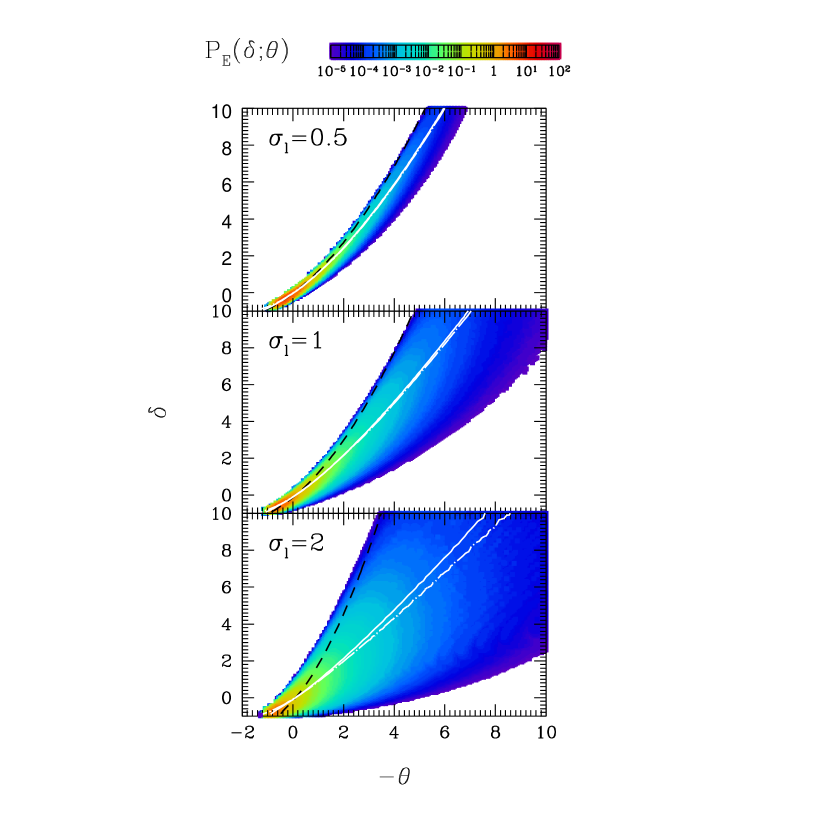
Figure 5: Contour plot of Eulerian joint PDF $P_{\scriptscriptstyle E}(\delta;\theta)$ as functions of $-\theta$ and $\delta$ from the ellipsoidal collapse model with linear external tide. In each panel, the solid and the dot-dashed lines respectively denote the conditional means $-[\theta]_{\delta}$ and $[\delta]_{\theta}$. The short-dashed lines represent the relation obtained from the spherical collapse model: $\sigma_{l}=0.5$(top); $\sigma_{l}=1$(middle); $\sigma_{l}=2$(bottom).

Finally, using the ellipsoidal collapse model with linear external tide, we examine the Eulerian joint PDF of local density and velocity-divergence evaluated at the same time, i.e., $P_{\scriptscriptstyle E}(\delta;\theta)$. In Figure 5, contour plots of joint PDF $P_{\scriptscriptstyle E}(\delta;\theta)$ for various linear fluctuation values $\sigma_{l}$ are depicted as function of $-\theta$ and $\delta$. This is the so-called density-velocity relation, which might be of observational interest in measuring the density parameter $\Omega_{\rm m}$ from the velocity-density comparison through the POTENT analysis (e.g., Bertschinger & Dekel, 1989). Along the line of this, theoretical works based on the Eulerian perturbation theory have attracted much attention, as well as the N-body study (e.g., Bernardeau, 1992a; Chodorowski & Lokas, 1997; Bernardeau et al., 1999). Based on the solution of the local approximation (36), one can easily calculate the perturbation series of velocity-density relation $[\theta]_{\delta}$ as function of local density and density-velocity relation $[\delta]_{\theta}$ as function of velocity-divergence, the leading-order results of which are expected to coincide with previous early works in the non-smoothing case, exactly. Beyond the perturbation analysis, Figure 5 reveals the general trend of the stochastic nature in the velocity-density relation. As increasing $\sigma_{l}$, the scatter becomes much broader and the conditional means $[\delta]_{\theta}$ (dot-dashed) and $[\theta]_{\delta}$(solid) does not coincide with each other. Of course, the one-to-one mapping obtained from the spherical collapse model (short-dashed) fails to match the both conditional means. These qualitative behavior is in fact consistent with the N-body results by Bernardeau et al. (1999) and the present model provides a simple way to derive the non-linear and stochastic velocity-density relation.

4 CONCLUSION AND DISCUSSION

In this paper, starting from a general theory of evolution of one-point PDFs, we derived the evolution equations for PDF and within a local approximation, consistent formal solutions of PDF are constructed in both the Lagrangian and the Eulerian frames (see eqs.[21][22] for Lagrangian PDFs and eqs.[32][33] with eqs.[27][30] for Eulerian PDFs). In order to reveal the stochastic nature arising from the multivariate Lagrangian dynamics, we further consider the Eulerian joint PDF $P_{\scriptscriptstyle E}(\delta,\theta;t)$ (eq.[36]) and the Lagrangian joint PDF $P_{\scriptscriptstyle L}(\delta,t;\delta^{\prime},t^{\prime})$ (eq.[38]). Then, adopting the spherical and the ellipsoidal collapse models as representative Lagrangian local dynamics, we explicitly evaluate the Eulerian PDFs, $P_{\scriptscriptstyle E}(\delta)$ and $P_{\scriptscriptstyle E}(\theta)$, as well as the joint PDFs. The results from the ellipsoidal collapse model show several distinct properties. While the PDF $P_{\scriptscriptstyle E}(\delta)$ almost coincides with the one-to-one mapping of the spherical collapse model, the tails of velocity-divergence PDF $P_{\scriptscriptstyle E}(\theta)$ largely deviate from those obtained from the spherical model. These behaviors have also been confirmed from the perturbative analysis of higher order moments. On the other hand, evaluating the Lagrangian joint PDF of local density, $P_{\scriptscriptstyle L}(\delta,t;\delta^{\prime},t^{\prime})$, a large scatter in the relation between the initial and the evolved density fields was found and their mean relation fails to match the one-to-one mapping of spherical collapse model. This remarkably reproduces the same situation in the N-body simulation. Therefore, the local approximation with ellipsoidal collapse model provides a simple and physically reasonable model of one-point statistics, consistent with the leading-order results of exact perturbation theory.

Since the present formalism described in section 2 is quite general, the approach does not restrict its applicability to the pressure-less cosmological fluid. Rather, one may apply to the various fluid systems in presence or absence of gravity. As mentioned in section 2.4, however, the applicability or the validity of local approximation of PDFs, in principle, sensitively depends on the choice of Lagrangian local dynamics. In the last section, simple and intuitive examples were examined for the illustrative purposes. The results indicate that the multivariate Lagrangian dynamics rather than the local model with a single variable can describe various statistical features of fluid evolution including the stochastic nature.

Perhaps, a straightforward extension of the present treatment is to include the effect of redshift-space distortion or projection effect, which is practically important for proper comparison with observation. Before addressing this issue, however, remember the most primarily importance of the smoothing effect. While the appropriate prescription for top-hat smoothing filter does exist in the local approximation with the spherical collapse model (e.g., Bernardeau, 1994b; Protogeros & Scherrer, 1997; Fosalba & Gaztañaga, 1998a), the smoothing effect on the approximation using ellipsoidal collapse model still needs to be investigated. This step is in particular a crucial task in order to construct a more physical prescription for one-point statistics of cosmic fields and the analysis is now in progress. The results will be presented elsewhere (Ohta, Kayo & Taruya, in preparation).

Appendix A ON NORMALIZATION CONDITION OF PDFs

In computing the PDFs from the local approximation with the spherical or the ellipsoidal collapse model, one may practically encounter the case when the evolved density at a finite elapsed time infinitely diverges for some regions in initial parameter space. To avoid the unphysical divergences, we restrict the integral over the entire initial parameter space appearing in the PDFs to some regions $V(t)$, in which the local density $\delta$ does not diverge. This modification slightly alters the normalization condition for both the Lagrangian and the Eulerian PDFs in section 2.4 and 2.5, which should be corrected in the following re-normalization procedure.

First of all, the initial distribution function $P_{\scriptscriptstyle I}({\mbox{\boldmath$p$}})$ should be re-normalized as

$$\tilde{P_{\scriptscriptstyle I}}({\mbox{\boldmath$p$}})=\frac{\displaystyle P_{\scriptscriptstyle I}({\mbox{\boldmath$p$}})}{\displaystyle\int_{V(t)}\prod_{i}dp_{i}\,P_{\scriptscriptstyle I}({\mbox{\boldmath$p$}})}.$$ (A1)

Then, the modification of Lagrangian PDFs is to replace the initial distribution $P_{\scriptscriptstyle I}({\mbox{\boldmath$p$}})$ with $\tilde{P_{\scriptscriptstyle I}}({\mbox{\boldmath$p$}})$, together with the change of the integral region. For example, the one-pint PDF $P_{\scriptscriptstyle L}(\delta)$ in equation (21) is modified as follows:

$$P_{\scriptscriptstyle L}(\delta;t)=\int_{V(t)}\prod_{i}dp_{i}\tilde{P_{\scriptscriptstyle I}}({\mbox{\boldmath$p$}})\,\,\delta_{D}(\delta-f({\mbox{\boldmath$p$}},t)).$$ (A2)

On the other hand, for the Eulerian PDFs, notice the fact that the re-normalization (A1) also affects the relation between $\delta$ and $f({\mbox{\boldmath$p$}},t)$ (see eq.[27]), which must be modified as

$$1+\tilde{g}({\mbox{\boldmath$p$}},t)\equiv\tilde{N}_{E}(t)\left\{1+f({\mbox{\boldmath$p$}},t)\right\}~{}~{};~{}~{}~{}~{}~{}~{}~{}\tilde{N}_{E}(t)\equiv\int_{V(t)}\prod_{i}dp_{i}\,\,\frac{\tilde{P_{\scriptscriptstyle I}}({\mbox{\boldmath$p$}})}{1+f({\mbox{\boldmath$p$}},t)}.$$ (A3)

Using this relation, the renormalized one-point PDFs (32) and (33) respectively become

$$P_{\scriptscriptstyle E}(\delta;t)=\frac{1}{1+\delta}\,\int_{V(t)}\prod_{i}dp_{i}\,\,\tilde{P_{\scriptscriptstyle I}}({\mbox{\boldmath$p$}})\,\,\delta_{D}(\delta-\tilde{g}({\mbox{\boldmath$p$}},t))$$ (A4)

for the PDF $P_{\scriptscriptstyle E}(\delta)$ and

$$P_{\scriptscriptstyle E}(\theta)=\int_{V(t)}\prod_{i}dp_{i}\,\,\frac{\tilde{P_{\scriptscriptstyle I}}({\mbox{\boldmath$p$}})}{1+\tilde{g}}\,\,\delta_{D}\left(\theta+\frac{1}{H(1+f)}\frac{df}{dt}+k\right)$$ (A5)

for the PDF $P_{\scriptscriptstyle E}(\theta)$. Here the variable $k$ is given by

$$k=-\frac{1}{\tilde{N}_{E}}\int_{V(t)}\prod_{i}dp_{i}\,\,\frac{1}{H(1+f)^{2}}\,\,\frac{df}{dt}\,\,\tilde{P_{\scriptscriptstyle I}}({\mbox{\boldmath$p$}}),$$ (A6)

under the approximation that the time evolution of $V$ is neglected, $\dot{V}/V\ll\dot{f}/(1+f)$. Similarly, the renormalized Eulerian joint PDF $P(\delta,\theta;t)$ corresponding to the expression (36) becomes

$$P_{\scriptscriptstyle E}(\delta,\theta;t)=\frac{1}{1+\delta}\int_{V(t)}\prod_{i}dp_{i}\,\,\tilde{P_{\scriptscriptstyle I}}({\mbox{\boldmath$p$}})\,\,\delta_{D}(\delta-\tilde{g})\,\delta_{D}\left(\theta+\frac{1}{H(1+f)}\frac{df}{dt}+k\right).$$ (A7)

Appendix B CUMULANTS FROM SPHERICAL AND ELLIPSOIDAL COLLAPSE MODELS

In this appendix, based on the local approximation with spherical and ellipsoidal collapse models, we briefly summarize the essence of the perturbation analysis for higher order moments of local density and velocity-divergence. The details of the calculation procedure including the effect of smoothing will be presented elsewhere (Ohta, Kayo & Taruya, in preparation). Here, we only present the results in non-smoothing case.

Let us write down the evolution equation for ellipsoidal collapse model. In an Einstein-de Sitter universe, equation (45) becomes

$$a^{2}\frac{d^{2}\alpha_{i}}{da^{2}}-\frac{a}{2}\frac{d\alpha_{i}}{da}=-\frac{3}{2}\alpha_{i}\left(\frac{1+\delta}{3}+\frac{b_{i}}{2}\delta+\lambda_{{\rm ext},i}\right).$$ (B1)

In this case, the linear growth rate $D$ is proportional to the scale factor $a$. Thus, the half length of principal axis $\alpha_{i}$ can be expanded by a power series of $a$:

$$\alpha_{i}=a\left(1-\sum_{j=1}\gamma_{i}^{(j)}a^{j}\right)$$ (B2)

Note that the initial conditions (49) and (50) state $\gamma_{i}^{(1)}=\lambda_{i}$. Hence, substituting the expression (B2) into (B1) and solving the evolution equation perturbatively, the coefficient $\gamma_{i}^{(j)}$ is systematically determined order by order and is expressed as the function of $\lambda_{i}$. Thus, the perturbative expansion of local density $\delta$ given by (47) is also expressed in terms of $\lambda_{i}$ :

$$f(\lambda_{i},a)=\frac{a^{3}}{\alpha_{1}\alpha_{2}\alpha_{3}}-1=\sum_{j=1}\,\delta^{(j)}(\lambda_{i})\,\,\,a^{j},$$ (B3)

with the corresponding boundary condition being $\delta^{(1)}=\lambda_{1}+\lambda_{2}+\lambda_{3}$.

Provided the function $f(\lambda_{i},a)$, one can calculate the $n$-th order moments of $\delta$ and $\theta$ as well as the normalization factor $N_{E}$, according to the one-point PDFs of local approximation, (32) and (33):

$$N_{E}= \int\prod_{i}\,d\lambda_{i}\,\,\frac{P_{\scriptscriptstyle I}(\lambda_{i})}{1+f(\lambda_{i})},$$ (B4)

$$\langle\delta^{n}\rangle_{\scriptscriptstyle E}= \int d\delta\ \delta^{n}\,\,P_{\scriptscriptstyle E}(\delta)=\int\prod_{i}d\lambda_{i}\,\,\frac{[N_{E}\{1+f(\lambda_{i},a)\}-1]^{n}}{N_{E}\{1+f(\lambda_{i})\}}P_{\scriptscriptstyle I}(\lambda_{i}),$$ (B5)

$$\langle\theta^{n}\rangle_{\scriptscriptstyle E}= \int d\theta\ \theta^{n}\,\,P_{\scriptscriptstyle E}(\theta)=\int\prod_{i}d\lambda_{i}\,\,\frac{1}{N_{E}(1+f)}\left(-\frac{a}{1+f}\frac{df}{da}-\frac{a}{N_{E}}\frac{dN_{E}}{da}\right)^{n}P_{\scriptscriptstyle I}(\lambda_{i}),$$ (B6)

where the function $P_{\scriptscriptstyle I}(\lambda_{i})$ denotes the PDF of initial parameter $\lambda_{i}$ given by (52).

Below, we separately present the perturbation results in each model. For the results of higher order moments, i.e., variance, skewness and kurtosis given by (53)–(58), numerical values of the perturbation coefficient are summarized in table 1 and the departure from the leading-order results are depicted in figure 3.

B.1 Ellipsoidal collapse model with linear external tide

If adopting the ellipsoidal collapse model with linear external tide (see eq.[48]), the perturbative expansion of local density, $\delta^{(n)}$ up to the fifth order becomes

$$\delta^{(1)} = \delta_{l},$$ (B7)

$$\delta^{(2)} = \frac{17}{21}\delta_{l}^{2}+\frac{4}{21}J_{1},$$ (B8)

$$\delta^{(3)} = \frac{341}{567}\delta_{l}^{3}+\frac{1538}{4725}\delta_{l}J_{1}+\frac{4}{405}J_{2},$$ (B9)

$$\delta^{(4)} = \frac{55805}{130977}\delta_{l}^{4}+\frac{952144}{2480625}\delta_{l}^{2}J_{1}+\frac{345088}{16372125}\delta_{l}J_{2}+\frac{12368}{363825}J_{1}^{2},$$ (B10)

$$\delta^{(5)} = \frac{213662}{729729}\delta_{l}^{5}+\frac{237342074}{621928125}\delta_{l}^{3}J_{1}+\frac{93363344}{3192564375}\delta_{l}^{2}J_{2}$$ (B11)

$$\ +\frac{52865818}{638512875}\delta_{l}J_{1}^{2}+\frac{135052}{34827975}J_{1}J_{2},$$

where $\delta_{l}$ denotes the linear fluctuation density given by $\delta_{l}=\lambda_{1}+\lambda_{2}+\lambda_{3}$. Here we introduced the quantities $J_{1}\equiv x^{2}+xy+y^{2}$ and $J_{2}\equiv(x-y)(2x+y)(x+2y)$ with the variables $x$ and $y$ being $x=\lambda_{1}-\lambda_{2}$ and $y=\lambda_{2}-\lambda_{3}$, respectively. Substituting the above expansion results into (B4), the normalization factor of Eulerian PDF becomes

$$N_{E}=1+\frac{69668}{3898125}\sigma_{l}^{4}+\cdots.$$ (B12)

Further, using the equations (B5) and (B6), one can obtain the variance, the skewness and the kurtosis defined in (53)–(58). For the variances of local density and velocity-divergence, the perturbative correction up to the two-loop order ${\cal O}(\sigma_{l}^{6})$ becomes

$$\sigma^{2} = \sigma_{l}^{2}+\frac{57137}{33075}\sigma_{l}^{4}+\frac{469828713881}{111739753125}\sigma_{l}^{6}+\cdots,$$ (B13)

$$\sigma_{\theta}^{2} = \sigma_{l}^{2}+\frac{8747}{11025}\sigma_{l}^{4}+\frac{154583563}{165540375}\sigma_{l}^{6}+\cdots.$$ (B14)

As for the skewness and the kurtosis, we obtain the results up to the one-loop order ${\cal O}(\sigma_{l}^{2})$:

$$S_{3} = \frac{34}{7}+\frac{646404856}{63669375}\sigma_{l}^{2}+\cdots,$$ (B15)

$$S_{4} = \frac{60712}{1323}+\frac{210688932175742}{782178271875}\sigma_{l}^{2}+\cdots,$$ (B16)

for the local density and

$$T_{3} = -\frac{26}{7}-\frac{333940984}{63669375}\sigma_{l}^{2}+\cdots,$$ (B17)

$$T_{4} = \frac{12088}{441}+\frac{17145801103334}{156435654375}\sigma_{l}^{2}+\cdots,$$ (B18)

for the velocity-divergence.

B.2 Ellipsoidal collapse model with non-linear external tide

In the case of the ellipsoidal collapse model with nonlinear external tide, the perturbative solution $\delta^{(n)}$ up to the fifth order becomes

$$\delta^{(1)} = \delta_{l},$$ (B19)

$$\delta^{(2)} = \frac{17}{21}\delta_{l}^{2}+\frac{4}{21}J_{1},$$ (B20)

$$\delta^{(3)} = \frac{341}{567}\delta_{l}^{3}+\frac{338}{945}\delta_{l}J_{1}+\frac{92}{3969}J_{2},$$ (B21)

$$\delta^{(4)} = \frac{55805}{130977}\delta_{l}^{4}+\frac{485288}{1091475}\delta_{l}^{2}J_{1}+\frac{234088}{4584195}\delta_{l}J_{2}+\frac{429728}{10696455}J_{1}^{2},$$ (B22)

$$\delta^{(5)} = \frac{213662}{729729}\delta_{l}^{5}+\frac{292398464}{638512875}\delta_{l}^{3}J_{1}+\frac{64182728}{893918025}\delta_{l}^{2}J_{2}$$ (B23)

$$\ +\frac{6541246}{59594535}\delta_{l}J_{1}^{2}+\frac{828974992}{96364363095}J_{1}J_{2}.$$

Then the normalization factor is

$$N_{E}=1+\frac{10844}{848925}\sigma_{l}^{4}+\cdots.$$ (B24)

The variances of local density and velocity-divergence up to the two-loop order become

$$\sigma^{2} = \sigma_{l}^{2}+\frac{439}{245}\sigma_{l}^{4}+\frac{3143785639}{695269575}\sigma_{l}^{6}+\cdots,$$ (B25)

$$\sigma_{\theta}^{2} = \sigma_{l}^{2}+\frac{145}{147}\sigma_{l}^{4}+\frac{1708470649}{1158782625}\sigma_{l}^{6}+\cdots.$$ (B26)

The results for the skewness and the kurtosis can be reduced to

$$S_{3} = \frac{34}{7}+\frac{1041064}{101871}\sigma_{l}^{2}+\cdots,$$ (B27)

$$S_{4} = \frac{60712}{1323}+\frac{941370178286}{3476347875}\sigma_{l}^{2}+\cdots,$$ (B28)

for the local density and

$$T_{3} = -\frac{26}{7}-\frac{2701112}{509355}\sigma_{l}^{2}+\cdots,$$ (B29)

$$T_{4} = \frac{12088}{441}+\frac{128186956538}{1158782625}\sigma_{l}^{2}+\cdots.$$ (B30)

for the velocity-divergence.

B.3 Spherical collapse model

In the case of spherical collapse model, the perturbative solutions of local density $f(\delta_{l})$ just corresponds to those obtained from the ellipsoidal collapse model simply setting $J_{1}=0$ and $J_{2}=0$, since the three initial parameters of principal axis $\lambda_{i}$ are identical. The cumulants are then calculated in similar way to the previous subsection except for the initial parameter PDF (44). The resultant normalization factor is

$$N_{E}=1+\frac{4}{21}\sigma_{l}^{2}+\frac{460}{43659}\sigma_{l}^{4}+\cdots.$$ (B31)

The variances of $\delta$ and $\theta$ become

$$\sigma^{2} = \sigma_{l}^{2}+\frac{1909}{1323}\sigma_{l}^{4}+\frac{344439415}{107270163}\sigma_{l}^{6}+\cdots,$$ (B32)

$$\sigma_{\theta}^{2} = \sigma_{l}^{2}-\frac{11}{147}\sigma_{l}^{4}+\frac{319159}{1324323}\sigma_{l}^{6}+\cdots.$$ (B33)

The skewness and the kurtosis respectively becomes

$$S_{3} = \frac{34}{7}+\frac{1026488}{101871}\sigma_{l}^{2}+\cdots,$$ (B34)

$$S_{4} = \frac{60712}{1323}+\frac{22336534498}{83432349}\sigma_{l}^{2}+\cdots,$$ (B35)

for the local density and

$$T_{3} = -\frac{26}{7}-\frac{613936}{101871}\sigma_{l}^{2}+\cdots,$$ (B36)

$$T_{4} = \frac{12088}{441}+\frac{10081115810}{83432349}\sigma_{l}^{2}+\cdots,$$ (B37)

for the velocity-divergence.

Table 1: Coefficients of perturbative correction for the density and the velocity-divergence in one-point statistics from the spherical and the ellipsoidal collapse models (see eqs.[53]–[58]).

	SCM${}^{~{}{\dagger}}$	ECM1${}^{~{}{\ddagger}1}$	ECM2${}^{~{}{\ddagger}2}$
$s_{2,4}$	$1.44$	$1.73$	$1.79$
$s_{2,6}$	$3.21$	$4.20$	$4.52$
$S_{3,0}$	$4.86$	$4.86$	$4.86$
$S_{3,2}$	$10.08$	$10.15$	$10.22$
$S_{4,0}$	$45.89$	$45.89$	$45.89$
$S_{4,2}$	$267.72$	$269.36$	$270.79$
$s_{2,4}^{\theta}$	$-0.075$	$0.79$	$0.99$
$s_{2,6}^{\theta}$	$0.24$	$0.93$	$1.47$
$T_{3,0}$	$-3.71$	$-3.71$	$-3.71$
$T_{3,2}$	$-6.03$	$-5.24$	$-5.30$
$T_{4,0}$	$27.41$	$27.41$	$27.41$
$T_{4,2}$	$120.83$	$109.60$	$110.62$

^† Spherical collapse model
^‡1 Ellipsoidal collapse model with linear external tide
^‡2 Ellipsoidal collapse model with non-linear external tide

Figure 2: Eulerian one-point PDF, $P_{\scriptscriptstyle E}(\delta)$(top) and $P_{\scriptscriptstyle E}(\theta)$(bottom) for the ellipsoidal collapse model with linear external tide (thick lines) and for the spherical collapse model (thin lines). In each panel, solid, long-dashed and short-dashed lines represent the results in cases with the linear rms fluctuation $\sigma_{l}=0.5$, $1$ and $2$, respectively.

Figure 3: Departures of the variance, the skewness and the kurtosis of local density(left) and the velocity-divergence(right) from the tree-level perturbation results. While the variances $\sigma^{2}$ and $\sigma_{\theta}^{2}$ are calculated up to the sixth order of the linear rms fluctuation $\sigma_{l}$, the perturbation results for the skewness $S_{3},\,T_{3}$ and the kurtosis $S_{4},\,T_{4}$ are obtained up to the one-loop order, ${\cal O}(\sigma_{l}^{2})$ (see Appendix B in detail). In each panel, the dashed and the dotted lines indicate the results obtained from the ellipsoidal collapse model with linear external tide and nonlinear external tide, respectively. For comparison, the results from the spherical collapse model are also shown in solid lines.

References

- Bardeen et al. (1986) Bardeen, J. M., Bond, J. R., Kaiser, N., & Szalay, A. S. 1986, ApJ, 304, 15
- Bartelmann & Schneider (2001) Bartelmann, M., & Schneider, P. Phys.Rep., 340, 291
- Bernardeau (1992a) Bernardeau, F. 1992, ApJ, 390, L61
- Bernardeau (1992b) Bernardeau, F. 1992, ApJ, 392, 1
- Bernardeau (1994a) Bernardeau, F. 1994a, ApJ, 427, 51
- Bernardeau (1994b) Bernardeau, F. 1994b, A&A, 291, 697
- Bernardeau & Kofman (1995) Bernardeau, F.,& Kofman,L. 1995, ApJ, 443, 479
- Bernardeau et al. (1999) Bernardeau, F., Chodorowski, M. J., Lokas, E. L., Stompor, R., Kudlicki, A. 1999, MNRAS, 309, 543
- Bertschinger & Dekel (1989) Bertschinger, E., & Dekel, A. 1989, ApJ, 336, L5
- Bond & Myers (1996) Bond, J. R.,& Myers, S. T. 1996, ApJS, 103, 1
- Bouchet et al. (1993) Bouchet, F., Strauss, M. A., Davis, M., Fisher, K. B., Yahil, A., & Huchra, J. P. 1993, ApJ, 417, 36
- Chen et al. (1989) Chen, H., Chen, S., & Kraichnan, R. H. 1989, Phys.Rev.Lett. 63, 2657
- Chodorowski & Lokas (1997) Chodorowski, M. J., & Lokas, E. L. 1997, MNRAS, 287, 591
- Dekel & Lahav (1999) Dekel, A., & Lahav, O. 1999, ApJ, 520, 24
- Doroshkevich (1970) Doroshkevich, A. G. 1970, Astrofizika, 6, 581
- Fosalba & Gaztañaga (1998a) Fosalba, P., & Gaztañaga, E. 1998a, MNRAS, 301, 503
- Fosalba & Gaztañaga (1998b) Fosalba, P., & Gaztañaga, E. 1998b, MNRAS, 301, 535
- Goto & Kraichnan (1993) Goto, T., & Kraichnan, R. H. 1993, Phys.Fluids A, 5, 445
- Hamilton (1985) Hamilton, A. J. S. 1985, ApJ, 292, L35
- Juszkiewicz et al. (1995) Juszkiewicz, R., Weinberg, D. H., Amsterdamski, P., Chodorowski, M., & Bouchet, F. 1995, ApJ, 442, 39
- Kayo et al. (2001) Kayo, I., Taruya, A., & Suto, Y. 2001, ApJ, 561, 22
- Kofman et al. (1994) Kofman, L., Bertschinger, E., Gelb, J. M., & Dekel, A. 1994, ApJ, 420, 44
- Protogeros & Scherrer (1997) Protogeros, Z. A. M., & Scherrer, R. J. 1997, MNRAS, 284, 425
- Scherrer & Gaztañaga (2001) Scherrer, R. J., & Gaztañaga, E. 2001, MNRAS, 328, 257
- Taruya et al. (1999) Taruya, A., Koyama, K., & Soda, J. 1999, ApJ, 510, 541
- Taruya & Suto (2000) Taruya, A., & Suto, Y. 2000, ApJ, 542, 577
- Taruya et al. (2002a) Taruya, A., Takada, M., Hamana, T., Kayo, I., & Futamase, T. 2002, ApJ, 571, 638
- Taruya et al. (2002b) Taruya, A., Hamana, T., & Kayo, I. 2002, MNRAS, in press (astro-ph/0210507)
- Taylor & Watts (2000) Taylor, A. N., & Watts, P. I. R. 2000, MNRAS, 314, 92