A Full-Sky H-alpha Template for Microwave Foreground Prediction

Abstract

A full-sky H$\alpha$ map with $6^{\prime}$ (FWHM) resolution is presented. This map is a composite of the Virginia Tech Spectral line Survey (VTSS) in the north and the Southern H-Alpha Sky Survey Atlas (SHASSA) in the south. The Wisconsin H-Alpha Mapper (WHAM) survey provides a stable zero-point over 3/4 of the sky on a $1^{\circ}$ scale. This composite map can be used to provide limits on thermal bremsstrahlung (free-free emission) from ionized gas known to contaminate microwave-background data. The map is available on the WWW for public use.

Subject headings: dust, extinction — ISM: clouds — HII regions

1 INTRODUCTION

Over the last 5 years, 3 surveys of the H$\alpha$ line (the 3-2 transition in neutral atomic H – used as a tracer of ionized gas) have revolutionized our knowledge of the warm ionized medium. Two high resolution surveys reveal supernova remnants, supershells, and filamentary structure in the diffuse ISM with breathtaking detail. A third survey, lower in spatial resolution but with velocity information, has provided a dramatic picture of the kinematics of the ISM over 3/4 of the sky.

To the microwave astronomer, these surveys can play another role: tracing the free-free emission of the Galaxy. Cosmic microwave background (CMB) anisotropy experiments have long detected ISM emission as a foreground at $\sim 10-50{\rm~{}GHz}$ (COBE, Kogut et al.  1996; Saskatoon, de Oliveira-Costa et al.  1997; OVRO, Leitch et al.  1997; 19GHz survey, de Oliveira-Costa et al.  1998; Tenerife, de Oliveira-Costa et al.  1999). In some cases this ISM-correlated emission has been presumed to be free-free or synchrotron emission Kogut et al. (1996); in other cases, electric dipole emission Draine & Lazarian (1998) from rapidly rotating dust grains is suspected de Oliveira-Costa et al. (1999); Finkbeiner et al. (2002). With the increasing capabilities of current and future microwave experiments (CBI, Mason et al.  2002; DASI, Halverson et al.  2002; MAP, Bennett et al.  1997) a more thorough understanding of Galactic foreground emission will become increasingly important for cosmological work.

Now that the H$\alpha$ data are public we have combined these 3 surveys into a moderate resolution ($6^{\prime}$) full-sky well-calibrated composite map, optimized for use as a free-free template. Version 1.1 of this map, along with software to access it, is available on the World Wide Web.

2 THE DATA

The full-sky composite H$\alpha$ map is comprised of three wide-angle surveys, two at high resolution with poorly determined zero-point calibrations, and one at low resolution with a stable zero-point. The data used here were downloaded in December, 2001 from the web sites of VTSS, SHASSA, and WHAM.

2.1 VTSS

The Virginia Tech Spectral line Survey (VTSS) is a survey of the northern hemisphere with the Spectral Line Imaging Camera (SLIC) which is a fast $(f/1.2)$ CCD camera with a narrow bandpass (17Å) H$\alpha$ filter as well as a continuum filter. The CCD has a quantum efficiency of 80% at 6500Å. Survey images have $1.6^{\prime}$ pixels in $385\times 385$ images with a usable radius of 5 degrees from the center of each pointing. The fast optics and low noise CCD result in sub-Rayleigh sensitivity at confusion limited levels Dennison et al. (1998). At present, 107 fields have been released on the VTSS web site. As more are released, we will incorporate them into future versions of this map.

2.2 SHASSA

The complimentary effort in the south is the Southern H-Alpha Sky Survey (SHASSA; Gaustad et al.  2001), using a small camera at Cerro Tololo Inter-American Observatory (CTIO). The survey consists of 542 fields of $13^{\circ}\times 13^{\circ}$ spaced every $10^{\circ}$ on each pass. The two passes are shifted by $5^{\circ}$ in each coordinate, covering the southern $\delta<20^{\circ}$ sky twice. Each image is approximately 1k$\times$1k with $47^{\prime\prime}$ pixels. The sensitivity per pixel is $\sim 2$ Rayleigh, similar to VTSS. The $5^{\circ}$ offset between the passes allows one to discard the corners of the images, which are more difficult to calibrate. The SHASSA survey is complete, and is available on the web.

2.3 WHAM

The Wisconsin H-Alpha Mapper (WHAM) Northern Sky Survey (Reynolds, Haffner, & Madsen 2002) consists of 37,565 spectra obtained with a dual etalon Fabry-Perot spectrometer on a 0.6m telescope at Kitt Peak. The velocity resolution of $12{\rm~{}km/s}$ makes possible the removal of the geocoronal H$\alpha$ emission, providing a stable zero-point unavailable in the other two surveys. Velocity coverage is approximately $-100<v_{LSR}<80$ km/s and includes all significant H$\alpha$ emission along most lines of sight. The survey pointings are on a grid with $1^{\circ}$ spacing, undersampling the instrument’s $1^{\circ}$ diameter tophat beam (Haffner, Reynolds, & Tufte 2003).

3 PROCESSING STEPS

Essentially the same steps are followed for VTSS and SHASSA, except for the PSF (point spread function) wing masking for SHASSA. In this section we describe the treatment of stellar artifacts and the zero-point calibration using WHAM, compare resulting data in the VTSS / SHASSA overlap area, define an error map, and describe the reprojection of the surveys to a full sky Cartesian grid.

3.1 Stellar Artifacts

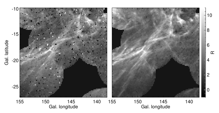
Figure 1: VTSS images zero-pointed to WHAM without (left) and with (right) point source removal.

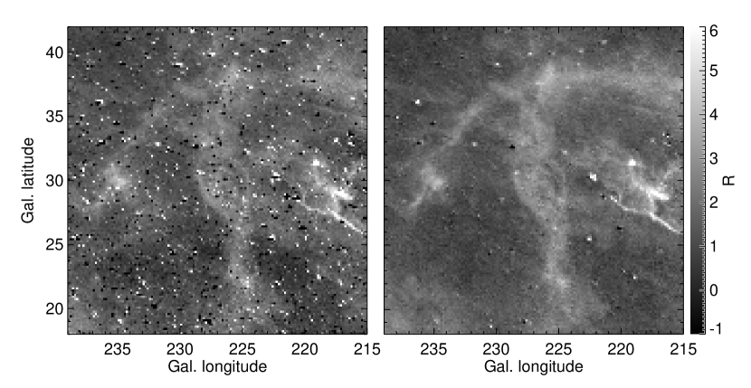
Figure 2: SHASSA images zero-pointed to WHAM without (left) and with (right) point source removal. All remaining stellar artifacts have the BRT_OBJ bit set in the bitmask.

The VTSS and SHASSA surveys have already produced “continuum-subtracted” images, meaning that a properly scaled continuum image has been subtracted from the narrow-band H$\alpha$ image to remove stars. Because of variations in PSF and stellar color, there are positive and negative residual ghosts in the subtracted image for $V\lesssim 11$ stars. These are small compared to the original stellar contamination (typically $10-20\%$) but large compared to some of the ISM structure. Removing these without damaging the real structure is our challenge.

The poorly subtracted stars are difficult to locate in the subtracted image, but are readily found in the continuum image with the well-known DAOfind algorithm created by Peter Stetson, as implemented in IDL by Wayne Landsman. The continuum images provided with the SHASSA survey are not generally co-registered with the H$\alpha$ images, and VTSS provides no continuum images at all, so for source detection we simply used as a continuum image the difference between the (already) co-registered H$\alpha$ images and “continuum-corrected” H$\alpha$ images. The sources identified in these images are then removed from the continuum-corrected image by linear interpolation to the unmasked parts of an annulus around them, with $3\sigma$ outlier rejection. This allows the fit to follow the gradient of any underlying ISM structure. The radius of the replaced region is 2 pixels (about $1.5^{\prime}$ for SHASSA, $3^{\prime}$ for VTSS), expanded to 3.5 pixels for Tycho $V\lesssim 9{\rm~{}mag}$. For bright stars a region of radius $16^{\prime}$, $20^{\prime}$, and $30^{\prime}$ is flagged in the BRT_OBJ mask bit for star brighter than Tycho V of 5.5, 3, and $1.5{\rm~{}mag}$ respectively. Because many of these bright stars reside within complicated H II regions, it would be reckless to interpolate over such large areas of the map. However, the remaining residuals from stellar subtraction mean that these regions should be excluded from statistical studies. The BRT_OBJ bit is only set in the SHASSA area; the outer wings of the VTSS PSF are better behaved so no such mask is necessary. Visual inspection of several fields indicates that the algorithm works well and finds stars while ignoring real ISM structure. Figure 1 shows VTSS data with and without the point source subtraction; Figure 2 displays the same comparison for SHASSA.

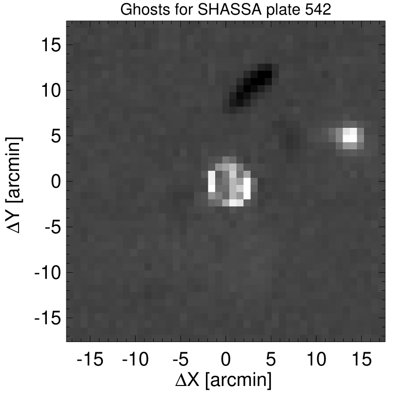
Figure 3: SHASSA continuum-subtracted PSF wing pattern for plate 542. The positive ghost is caused by an internal reflection in the H$\alpha$ filter. The negative ghost is a reflection in the continuum filter. This pattern is typical, and is fairly constant throughout the survey, but we determine it independently for each SHASSA field. In some fields it is rotated by 180 degrees.

In the case of the SHASSA survey, the wings of the PSF are not well behaved. Imperfections in the filters cause “transmissive” ghosts near bright objects (Gaustad et al.  2001, §2.4). The ghosts in the narrow-band and continuum images are displaced, causing a defocused positive and negative ghost to appear in the wings of the continuum-subtracted PSF. The PSF is determined independently for each image, and found to be quite stable (Figure 3). Rather than attempting to deconvolve this PSF over the whole image, we simply determine which pixels are deviant and mask those near known objects. A cut of Tycho $V<7{\rm~{}mag}$ for stars was chosen by inspection, and the same mask (determined plate by plate) is then applied to all bright stars on a given plate.

The 100 brightest galaxies in the sky can also be seen in the map, but the flux from these is usually comparable to other remaining artifacts, so they are not removed. Many bright compact sources remaining in the maps are not artifacts at all, but planetary nebulae, for example NGC 246 at $(l,b)=(118.86,-74.71)$ and NGC 7293 (the Helix Nebula; see Speck et al.  2002) at $(36.14,-57.15)$. Such objects can be very bright (500R or more) but pains have been taken to not remove them from the map. Statistical comparisons with microwave data sets may want to mask these out and handle them separately.

Saturated pixels in bright stars require special handling. Bleed trails are present in both VTSS and SHASSA, but because of the preprocessing done upstream from the publicly released data, identification of saturated pixels is not trivial. Saturation is identified by taking the union of all pixels above a threshold, and those pixels with a second-difference in the direction orthogonal to the bleed trails above a threshold. This mask is then extended for 2 pixels in all directions to deal with nearby contamination. The neighboring pixels in directions perpendicular to the bleed direction are used for interpolation across the masked pixels. In most cases this yields acceptable results, even in the presence of real structure. The brightest few stars in the SHASSA region have bleed trails of different length in each of 5 exposures, so it is not always possible to remove these perfectly from the combined data. A few sections of bleed trails remain in the map around the brightest stars. A full re-analysis of the raw data would provide the required information, and may be attempted if these few remaining artifacts are found to compromise the scientific content of the present map.

In only a few places (e.g. Orion) the H$\alpha$ image itself has bleed trails. These regions must be handled on a case by case basis, and masked to indicate no processing should be done. No processing was done on the LMC, SMC, or M31 for similar reasons. These pixels have the “big_obj” mask bit set.

3.2 The WHAM zero point

Broadband surveys such as SHASSA and VTSS have an uncertain zero point because of smooth foreground contamination from geocoronal H$\alpha$ emission. The spectral resolution of WHAM allows removal of this foreground emission which is often brighter than the signal of interest. Note however that the WHAM data cover velocities $-100<v_{LSR}<80$ km/s and there is significant H$\alpha$ emission at $v_{LSR}>80$ km/s over a small part of the sky. We have estimated an upper bound on the error thus introduced by assuming that the intensity in the 80 km/s velocity bin is constant for $80<v_{LSR}<120$ km/s. Any WHAM pointing for which this upper bound exceeds both 0.2R and 10% has bit 7 (HI_VEL) set in the bit mask. Apart from this 0.5% of the sky, WHAM can provide the correct zero-point for high resolution images on one degree scales.

Because the WHAM survey is undersampled ($1^{\circ}$ diameter beams on a $1^{\circ}$ spacing) it does not contain enough information for an unambiguous solution, but the following prescription is reasonable, and produces an aesthetically pleasing map consistent with reality.

We approximate the WHAM beam to be a smoothed tophat with the form

$$W(r)=\frac{1}{\exp[(r-r_{0})/r_{s}]+1}$$ (1)

where $r$ is the angular distance from the beam center, $r_{0}$ is $1/2$ degree, and $r_{s}$ is a smoothing term set to $1/40$ degree. The smoothing is desirable because it makes the WHAM beam fully sampled in the raw H$\alpha$ images during convolution.

Each VTSS image is convolved with the WHAM beam centered on each WHAM pointing. The WHAM value is then subtracted (a floor of $-0.1$R is imposed on a few spurious WHAM measurements), yielding a set of differences, one for each WHAM pointing. Each WHAM pointing is then assigned a Gaussian (FWHM = $1^{\circ}$) weight used to interpolate the zero-point difference, which is then subtracted from the VTSS image. Again, this solution is not unique, nor strictly correct. A bandlimited WHAM-like data set could be interpolated exactly with sinc interpolation, leaving no ambiguity, but no such data exist at this time. The SHASSA images are processed in the same way, with the additional constraint that the corners of the images ($r>500$ pixels), which are systematically biased, are smoothly de-weighted.

Some outlier rejection is required in the above algorithm. Very bright sources can have a large difference residual, resulting in dark halos in the final map. Such differences, if they deviate by more than 3 R from the median of neighboring differences, are set to that median. This is justified because it removes unphysical halos and the error thus introduced in the bright pixels is fractionally very small.

3.3 Reprojection

Full sky maps, masks, and weight arrays are generated for the three surveys at a resolution of $6^{\prime}$. This smoothing is acceptable for a CMB free-free template because $6^{\prime}$ is higher resolution than current or planned low-frequency CMB data sets (even Planck HFI will only be $5^{\prime}$ FWHM) and is convenient for comparisons with the $6^{\prime}$ FWHM Schlegel, Finkbeiner, & Davis (1998; hereafter SFD98) dust map.

We use a full sky Cartesian Galactic $(l,b)$ projection with $8640\times 4320$ pixels ($2.5^{\prime}$ square pixels at $b=0$). Each of the 542 SHASSA and 107 VTSS source images is gaussian smoothed prior to projection, so that it will be well sampled ($2.4^{\prime}$ per FWHM) when reprojected. Then the pixel centers from the destination image are transformed to $(x,y)$ positions on the source image, where a value is obtained for each via bilinear interpolation. Because the smoothed source image is heavily oversampled, the form of interpolation is not important. An apodized weight map for each source image is also used so that subtle differences in the zero-levels in each image are blended smoothly and do not create sharp boundaries in the final image.

The WHAM survey itself must also be reprojected, so as to fill in regions of the sky where no SHASSA or VTSS data are available. A Delaunay triangulation is performed on the 37565 WHAM pointings and the IDL trigrid function Renka (1983) is used to interpolate values for every pixel. Naturally, the interpolation over the southern sky ($\delta\lesssim 30^{\circ}$) is undesirable and must be masked. We extend the WHAM pointing grid to cover the southern area, set these “mock” pointings to zero weight, and interpolate with the same Delaunay triangulation used for the data. Any pixels with weight less than unity after interpolation are masked out.

Weighting for the composite map is defined such that if SHASSA data are available (64.0% of the sky), they are used. Failing SHASSA, VTSS is used (11.7%), and WHAM fills in the remaining 24.3%. The composite map is shown in Figure 4 and the bitmask in Figure 5. Because the images have been zeroed to WHAM (except for 23.8% of the southern sky), boundaries between the high resolution images and WHAM are as smooth as can be expected, but the sudden jump in resolution can result in strange behavior of bright sources near the boundary. It would be far better to have the remaining VTSS data, and these data will be incorporated as soon as they are made public.

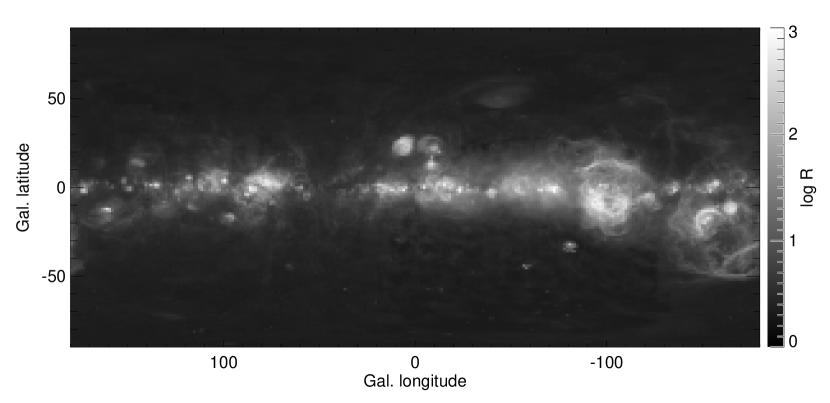
Figure 4: The composite H$\alpha$ map.

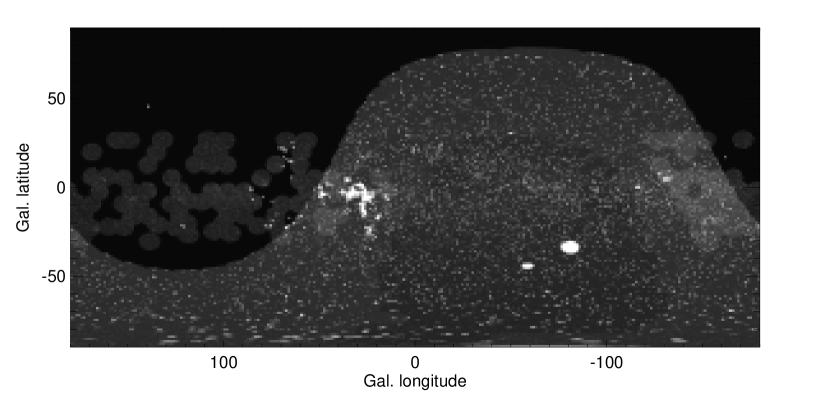
Figure 5: Bit mask for the composite H$\alpha$ map. The Boundaries of the 3 surveys are evident, as well as the masked point sources. The two largest white regions are the Magellanic Clouds. The bit mask is described in Table 2.

Figure 6: Flux difference (R) of SHASSA (convolved with WHAM beam) minus WHAM (integrated over $-80<v_{LSR}<80$ km/s) for every WHAM pointing with HI_VEL flag not set, vs. WHAM (in log R). The lines are $\pm(1$R + 10%) error.

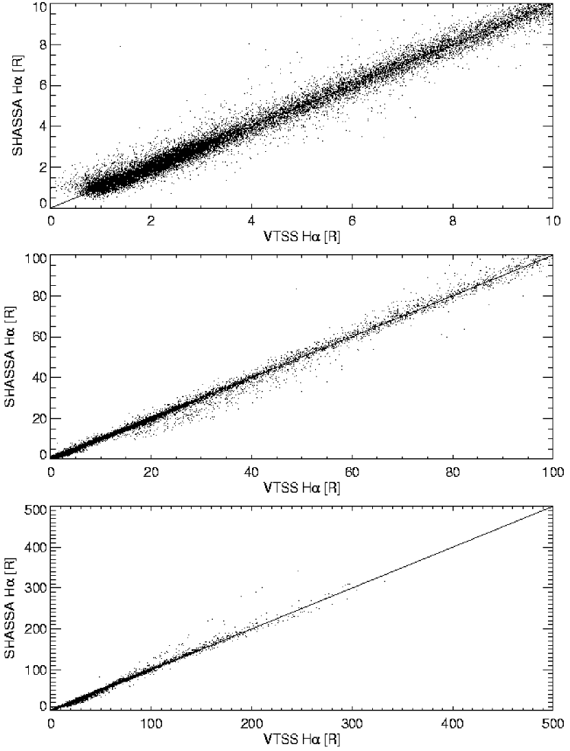
Figure 7: Comparison of VTSS and SHASSA in the overlap region for 3 different plot ranges. The WHAM zero point has been applied to both surveys on a 1 degree scale. For the diffuse ISM (fainter than 10R) the agreement is excellent with a scatter of $\sim 0.3$R. Agreement is generally good even in the brightest regions of the sky (see §3.4).

3.4 Photometric calibration

The overlap regions between the 3 surveys provide useful information about relative photometric calibration. The SHASSA zero point is fairly good even before correction to WHAM zero point described in §3.2, so a direct comparison of the two is straightforward. The SHASSA minus WHAM difference is plotted in Figure 6, where each point represents SHASSA flux integrated over a WHAM beam minus WHAM data. The overplotted lines represent residuals of $\pm(1$R + 10%) error. Evidently the calibration agreement is much better than 10%, in agreement with Gaustad et al.  (2001).

Because the VTSS maps were released with an arbitrary zero point, it is more convenient to check their calibration against SHASSA directly in the overlap region, after tying both surveys down to WHAM. Gaustad et al.  found VTSS to be fainter in one overlap region by a factor of 1.25. This same factor was applied to all VTSS data before tying down to WHAM, and the resulting agreement between VTSS and SHASSA is good (Figure 7). For faint values, the two maps agree well, with slope unity and a scatter of $\sim 0.3$R. Brighter than about 20R more outliers are evident, but agreement remains good even in the brightest parts of the sky. The estimate of 10% overall calibration error described in §3.5 relies on the calibration of SHASSA photometry to the planetary nebula photometry of Dopita & Hua (1997), which is claimed to be good to $\sim 5\%$.

The SHASSA data were never corrected for atmospheric extinction, because the correction is estimated to be small by Gaustad et al.  (2001). They measure an extinction coefficient of $k=0.082$ mag/airmass for H$\alpha$. Since the mean airmass of observation for SHASSA fields is always less than 1.6, this effect is less than 5% peak to peak. However, the average atmospheric absorption has been removed from the data by calibration to the Dopita & Hua sources, which have been corrected to zero airmass.

3.5 Error Map

It is nearly impossible to produce an error map for the composite data that will be meaningful for every application. Each processing step described above imprints another layer of covariances on the errors in the final map, and without full knowledge of these covariances, statistical studies (e.g. based on $\chi^{2}$) will be suspect.

Nevertheless, it is possible to estimate the uncertainty in a single pixel on the sky, resulting from the WHAM zero point, the VTSS/SHASSA CCD readout noise, Poisson noise from atmospheric light in the H$\alpha$ filter, and calibration errors. Note that Poisson errors from the Galactic H$\alpha$ are negligible in the final (smoothed) maps, being dominated by calibration uncertainty in bright regions and by readout noise and foreground Poisson errors in faint regions.

The estimated uncertainty in each pixel is given by

$$\sigma=\sigma_{W}+N+CI(H\alpha)$$ (2)

where $\sigma_{W}$ is the error map from the WHAM data, interpolated in the same way as the WHAM intensities; $N$ is the estimated readout noise plus sky noise of the VTSS and SHASSA surveys (after smoothing to a $6^{\prime}$ FWHM PSF); and C is the fractional calibration uncertainty of the VTSS and SHASSA surveys. Within the WHAM survey area, $\sigma_{W}$ is typically 0.03 R. For pixels outside the WHAM area or with the HI_VEL mask bit set, $\sigma_{W}$ is set to 1R to reflect the zero-point uncertainty in the southern data estimated by inspection. The WHAM data products have error set to zero for pointings contaminated by nearby stars; in these cases we interpolate nearby error values as the correlated systematics dominate any random measurement errors.

It is important to note that the error map does not reflect anything about artifacts in the map, caused by saturation bleed trails, very bright stars, etc. For these, please refer to the bitmask, especially the bright object bit (32) which indicates likely contamination of these pixels by bright stars or galaxies.

4 SUGGESTIONS FOR USE

In this section we describe the data format of the composite H$\alpha$ map, provide conversion factors from Rayleighs to EM and free-free intensity, and discuss the effects of dust extinction on the data.

4.1 Projections

The H$\alpha$ map, error map, and bitmask, are provided in two formats: a simple Cartesian Galactic longitude and latitude projection ($8640\times 4320$ pixels) and an Nside = 1024 HEALPIX (Górski et al.  1998) sphere, an equal area projection of the sphere popular within the CMB community. The HEALPIX projection has 12,582,912 equal area pixels ($3.4^{\prime}$ on a side) while the Cartesian projection has square $2.5^{\prime}$ pixels on the equator, with distortions at higher Galactic latitude. The Cartesian projection is simple, but we encourage the use of a FITS astrometry package to decipher the astrometric information in the file header to avoid confusion. Both maps are presented in units of Rayleighs, where 1R = $10^{6}/4\pi$ photons ${\rm cm^{-2}s^{-1}sr^{-1}}$.

The Cartesian projection is the “native” projection of the composite map, and the HEALPIX map is derived from it. The Cartesian map, mask and error map are in the files Halpha_map.fits, Halpha_mask.fits, and Halpha_error.fits, respectively.

The zero-indexed fractional pixel indices (suitable for interpolation) are

$$x=4319.5-24l$$ (3)

$$y=2159.5+24b$$ (4)

for $(l,b)$ in degrees and $-180^{\circ}<l<180^{\circ}$. Note that $l=180^{\circ}$ is mapped to $x=-0.5$, i.e. the average of column 0 and column 8639. Likewise, the Galactic north and south poles are mapped to $y=4319.5$ and $y=-0.5$ respectively. Any interpolation code needs to interpolate over these singularities properly.

4.2 Estimating Free-Free from H$\alpha$

H$\alpha$ and free-free are both tracers of the emission measure, $EM=\int n_{e}^{2}dl$. An EM of $1{\rm~{}cm^{-6}~{}pc}$ corresponds to $0.361(T/10^{4}{\rm~{}K})^{-0.9}$ R for $T<26000{\rm~{}K}$ (Kulkarni & Heiles).

The emission coefficient $j_{\nu}$ for free-free, with electrons assumed to interact with ions of charge $Z_{i}e$ and number density $n_{i}$ is

$$j_{\nu}=5.44\times 10^{-16}\frac{g_{ff}Z_{i}^{2}n_{e}n_{i}}{T^{1/2}}e^{-h\nu/kT}{\rm Jy~{}sr^{-1}~{}cm^{-1}}$$ (5)

where $g_{ff}$ is the gaunt factor for free-free. For microwave frequencies, a useful approximation is

$$g_{ff}=\frac{3^{1/2}}{\pi}\left[\ln\frac{(2kT)^{3/2}}{\pi e^{2}\nu m_{e}^{1/2}}-\frac{5\gamma}{2}\right]~{}~{}~{}~{}~{}\nu_{p}\ll\nu\ll kT/h$$ (6)

where $\gamma$ is the Euler constant ($\gamma\approx 0.577$) and $\nu_{p}$ is the plasma frequency (Spitzer 1978, p. 58). For convenience, Table 1 provides coefficients for converting emission measure to free-free specific intensity ($I_{\nu}$) and brightness temperature ($T_{B}$). CMB experiments usually express their results in terms of $\Delta T$, the temperature difference relative to a 2.73K blackbody. Brightness temperature may be converted to this thermodynamic $\Delta T$ by multiplying by the “planckcorr” factor:

$${\rm Planckcorr}=\frac{(e^{x}-1)^{2}}{x^{2}e^{x}}$$ (7)

where $x=h\nu/k_{b}T_{CMB}$ and $T_{CMB}=2.73$. Table 1 displays these factors for the nominal frequencies of by three CMB satellites. Note that these factors are evaluated for the frequencies listed and are not integrated over the passbands, as should be done for a detailed analysis.

4.3 Ionization of Interstellar He

The helium fraction in the interstellar medium is approximately $Y=0.25$ by mass, or $n_{He}/n_{H}=0.083$. For calculation of the free-free enhancement provided by the singly ionized He, the relevant ratio is $R=N($He II$)/N($H II). We neglect doubly ionized He entirely. The free-free emission per H atom is increased by the extra electrons (factor of $R+1$) and by additional ions available (another factor of $Z^{2}R+1$ with $Z=1$ for singly ionized He) yielding an enhancement factor of $(R+1)^{2}=1.17$ for $R=0.083$ (equal ionization of He and H). However, the H$\alpha$ emission per H atom is also enhanced by a factor of $R+1$, so the ratio of free-free to H$\alpha$ is a factor of $R+1$. In general, the value of $R$ is less than the abundance ratio in the diffuse ISM.

Indeed the He ionization fraction, $\chi_{He}\equiv n_{He^{+}}/n_{He(total)}$, is found to be significantly less than unity in the diffuse WIM. Observations of the He I $\lambda 5876$ recombination line in two directions at low Galactic latitude yield $\chi_{He}\lesssim 0.27$ within warm, low-density regions in which the H is primarily ionized (Reynolds & Tufte 1995). Radio recombination lines provide an even tighter constraint of $\chi_{He}/\chi_{H}\lesssim 0.13$ in the diffused ionized medium of the Galactic interior Heiles et al. (1996). For ionization fractions this low, ionized helium is unlikely to provide an free-free enhancement of more than a few percent, so no correction has been made to the map. In parts of the sky where He is mostly ionized, a correction may be desirable.

4.4 Combining with SFD Dust Map

At high Galactic latitude H$\alpha$ is expected to be an excellent tracer of the warm electron emission measure, but at low latitude Galactic dust absorbs and scatters the H$\alpha$ photons so that the stated EM derived above is too low.

If the H$\alpha$ emitting gas is uniformly mixed with dust in a cloud with total optical depth $\tau$, the observed intensity is

$$I_{\nu,obs}=\frac{I_{\nu}}{\tau}\int_{0}^{\tau}d\tau^{\prime}e^{-\tau^{\prime}}=\frac{I_{\nu}}{\tau}(1-e^{-\tau})$$ (8)

In the limit of large $\tau$, the intensity is simply reduced by a factor of $\tau$.

The optical depth $\tau$ is computed by multiplying the SFD dust map, in units of $E(B-V)$ magnitudes reddening, by 2.65/1.086. This value is close to that obtained by evaluating the reddening law (Cardelli, Clayton, & Mathis 1989) for $R_{V}=3.1$ at 6563Å. The factor of $1.086=2.5\times\log_{10}e$ and converts magnitudes of extinction to optical depth.

The derivation of the reddening law coefficient of 2.65 given above involves careful consideration of the procedure used to calibrate the SFD map. The reddening map was calibrated with a sample of elliptical galaxies on the Landolt system (see SFD, Appendix B for details). Therefore, the CCM reddening law was multiplied by an elliptical galaxy spectrum times the system response (atmosphere at CTIO, telescope optics, filter, and RCA 3103A photomultiplier) defining the Landolt system to obtain the values in SFD Table 6. This yields the apparently inconsistent result that $A(V)/E(B-V)=3.315$ for Landolt B and V, and reddening law parameter $R_{V}=3.1$. This is actually fine, because $R_{V}$ in this context only provides a parameterization of the family of reddening laws, and is not literally $A(V)/E(B-V)$ for every choice of filters and source spectra. In order to use the SFD predictions in an internally consistent way, one must divide the reddening law value for 6563Å by the $E(B-V)$ computed by SFD, obtaining the value of 2.65 given above.

Obviously the approximation that the dust is uniformly mixed with the ionized gas along each line of sight will sometimes be poor. At the very least, the combination of the H$\alpha$ map and the SFD dust map provides a robust lower limit (dust behind) and upper limit (dust in front of warm gas) to the actual EM, as well as a “best guess” (uniform mixing). Future microwave data sets will show to what extent these approximations are valid.

5 SUMMARY

We have reprocessed the VTSS and SHASSA H$\alpha$ surveys to remove bleed trails, stellar residuals, and other artifacts, and calibrated them to the stable zero point of the WHAM survey on $1^{\circ}$ scales. These surveys have been combined into a well sampled $6^{\prime}$ (FWHM) full-sky map, available in two projections (Galactic Cartesian and Galactic HEALPIX). A bit mask summarizing the area coverage of each survey and the processing done on each pixel is also provided, as well as an error map. All of these data products are available to the public on the web.

This map is designed to have a stable zero point, minimal contamination from stellar residuals and other artifacts, and is well sampled (band-limited) to facilitate spherical harmonic transforms and resampling. These properties make the map more convenient than the original data sets as a microwave free-free template; however, certain sacrifices have been made. The most obvious is that the map is somewhat lower resolution than the maps released by the SHASSA and VTSS surveys. In a few places on the sky, usually near bright stars, real ISM structure has been mistakenly removed. Therefore, researchers interested in a specific region of the ISM should consult the surveys directly and take advantage of the full resolution data.

We strongly encourage users to cite the original references describing the three surveys, and include the acknowledgments requested by each of them.

The Virginia Tech Spectral-Line Survey (VTSS), the Southern H-Alpha Sky Survey Atlas (SHASSA), and the Wisconsin H-Alpha Mapper (WHAM) are all funded by the National Science Foundation. SHASSA observations were obtained at Cerro Tololo Inter-American Observatory, which is operated by the Association of Universities for Research in Astronomy, Inc., under cooperative agreement with the National Science Foundation. John Gaustad, Peter McCullough, Ron Reynolds, Matt Haffner, Bruce Draine, Ed Jenkins, David Schlegel, and Jonathan Tan provided helpful information. This research made use of the NASA Astrophysics Data System (ADS) and the The IDL Astronomy User’s Library at Goddard. Partial support was provided by NASA via grant NAG5-6734 (Wire). DPF is a Hubble Fellow supported by HST-HF-00129.01-A.

Table 1: Conversion Factors from EM to Free-Free

Experiment	$\nu$	$\lambda$	$g_{ff}$	$I_{\nu}$	$T_{B}$	$T_{thermo}$
	GHz	mm		${\rm~{}Jy~{}sr^{-1}}$	$\mu{\rm K}$	$\mu{\rm K}$
	(2)	(3)	(4)	(5)	(6)	(7)
COBE/DMR	31.5	9.52	4.058	68.65	2.255	2.313
	53.0	5.66	3.771	63.79	0.740	0.795
	90.0	3.33	3.479	58.84	0.237	0.290
MAP	22.0	13.64	4.256	72.00	4.849	4.909
	30.0	10.00	4.085	69.10	2.503	2.561
	40.0	7.50	3.926	66.42	1.353	1.410
	60.0	5.00	3.703	62.63	0.567	0.622
	90.0	3.33	3.479	58.84	0.237	0.290
Planck	30.0	10.00	4.085	69.10	2.503	2.561
	44.0	6.82	3.874	65.53	1.103	1.159
	70.0	4.29	3.618	61.19	0.407	0.461
	100.0	3.00	3.421	57.86	0.189	0.242
	143.0	2.10	3.224	54.51	0.0869	0.143
	217.0	1.38	2.994	50.60	0.0350	0.104
	353.0	0.85	2.726	46.04	0.0120	0.154
	545.0	0.55	2.486	41.96	0.00460	0.727
	857.0	0.35	2.237	37.69	0.00167	25.746

Note. — Col. (2): Nominal central frequency, in GHz. Col. (3): Corresponding wavelength, in mm. Col. (4): Gaunt factor for free-free, given in eq.(6). Col. (5): Specific intensity, $I_{\nu}$, corresponding to EM=1. Col. (6): The brightness temperature ($\mu$K) corresponding to EM=1. Col. (7): Brightness temperature multiplied by Planckcorr (eq. 7) to convert to thermodynamic $\Delta T$, assuming $T_{CMB}=2.73$K.

Table 2: Bitmask Values

Bit	Name	% Sky	Comments
0	WHAM	76.23	WHAM data used (Wisconsin)
1	VTSS	17.35	Virginia Tech Spectral line Survey
2	SHASSA	63.99	Southern Halpha Sky Survey Atlas
3	STAR	6.94	Star removed
4	SATUR	2.58	Saturated pixel nearby in continuum exposure
5	BRT_OBJ	1.90	Bright star/galaxy - measurements unreliable
6	BIG_OBJ	0.14	Position near LMC, SMC, or M31; no sources removed
7	HI_VEL	0.53	High Velocity in WHAM data

Note. — The bitmask contains important information about survey coverage (bits 0-2), artifact removal (3,4) or lack thereof (6) and reliability (5). The BRT_OBJ and BIG_OBJ masks in particular must be used for any full-sky statistical study. Regions with HI_VEL set may have WHAM zero-point errors of greater than 10% and 0.2R. An image of the bitmask is shown in Figure 5.

References

- Bennett et al. [1997] Bennett, C. L. et al. 1997, AAS, 191, #87.01
- Cardelli, Clayton, & Mathis [1989] Cardelli, J. A., Clayton, G. C., & Mathis, J. S. 1989 ApJ, 345, 245
- de Oliveira-Costa et al. [1997] de Oliveira-Costa, A., Kogut, A., Devlin, M. J., Netterfield, C. B., Page, L. A., Wollack, E. J. 1997, ApJ, 482, L17
- de Oliveira-Costa et al. [1998] de Oliveira-Costa, A., Tegmark, M., Page, L., Boughn, S. 1998, ApJ, 509, L9
- de Oliveira-Costa et al. [1999] de Oliveira-Costa, A. et al. 1999, ApJ, 527, L9
- Dennison et al. [1998] Dennison, B., Simonetti, J. H., & Topasna, G. 1998, Publications of the Astronomical Society of Australia, 15, 147.
- Dopita & Hua [1997] Dopita, M. A. & Hua, C. T. 1997, ApJS, 108, 515
- Draine & Lazarian [1998] Draine, B. T., & Lazarian, A. 1998b, ApJ, 508, 157
- Finkbeiner et al. [2002] Finkbeiner, D. P., Schlegel, D. J., Frank, C., & Heiles, C. 2002, ApJ, 566, 898
- Gaustad et al. [2001] Gaustad, J. E., McCullough, P. R., Rosing, W. & Van Buren, D. 2001, PASP, 113, 1326
- Górski et al. [1998] Górski, K. M., Hivon, E., & Wandelt, B. D. 1998 in Proceedings of the MPA/ESO Cosmology Conference Evolution of Large-Scale Structure eds. A.J. Banday, R.S. Sheth and L. Da Costa
- Haffner, Reynolds, & Tufte [2003] Haffner, L. M., Reynolds, R. J., Tufte, S. L. et al. 2003, in preparation
- Halverson et al. [2002] Halverson, N. W. et al. 2002, ApJ568, 38
- Heiles et al. [1996] Heiles, C., Koo, B.-C., Levenson, N. A., & Reach, W. T. 1996 ApJ, 462, 326
- Kogut et al. [1996] Kogut, A. et al. 1996, ApJ, 464, L5
- Leitch et al. [1997] Leitch, E. M., Readhead, A. C. S., Pearson, T. J., & Myers, S. T. 1997, ApJ, 486, L23
- [17] Mason, B. S. et al. 2002 astro-ph/0205384, submitted to ApJ
- Renka [1983] Renka, R. J., 1983, Oak Ridge National Laboratory Report ORNL/CSD-108
- [19] Reynolds, R. J., Haffner, L. M., & Madsen, G. J. 2002, in “Galaxies: The Third Dimension”, ASP Conf. Series Vol. 282, eds. M. Rosado, L. Binette, & L. Arias, in press
- Reynolds & Tufte [1995] Reynolds, R. J., & Tufte, S. L. 1995 ApJ, 439, L17
- SFD [98] Schlegel, D. J., Finkbeiner, D. P., & Davis M. 1998, ApJ, 500, 525 [SFD]
- Speck et al. [2002] Speck, A. K., Meixner, M., Fong, D., McCullough, P. R., Moser, D. E., & Ueta, T. 2002, AJ, 123, 346
- Spitzer [1978] Spitzer, L. 1978, Physical Processes in the Interstellar Medium, Wiley, New York