The resolved fraction of the Cosmic X–ray Background

Abstract

We present the X–ray source number counts in two energy bands (0.5–2 and 2–10 keV) from a very large source sample: we combine data of six different surveys, both shallow wide field and deep pencil beam, performed with three different satellites (ROSAT, Chandra and XMM–Newton). The sample covers with good statistics the largest possible flux range so far: [$2.4\times 10^{-17}-10^{-11}$] erg s^-1 cm^-2 in the soft band and [$2.1\times 10^{-16}-8\times 10^{-12}]$ erg s^-1 cm^-2 in the hard band. Integrating the flux distributions over this range and taking into account the (small) contribution of the brightest sources we derive the flux density generated by discrete sources in both bands. After a critical review of the literature values of the total Cosmic X–Ray Background (CXB) we conclude that, with the present data, the $94.3_{-6.7}^{+7.0}\%$ and $88.8_{-6.6}^{+7.8}\%$ of the soft and hard CXB can be ascribed to discrete source emission. If we extrapolate the analytical form of the Log N–Log S distribution beyond the flux limit of our catalog in the soft band we find that the flux from discrete sources at $\sim 3\times 10^{-18}$ erg s^-1 cm^-2 is consistent with the entire CXB, whereas in the hard band it accounts for only $93\%$ of the total CXB at most, hinting for a faint and obscured population to arise at even fainter fluxes.

1 Introduction

The Cosmic X–ray Background (CXB) origin and nature have attracted the attention of astronomers since its discovery (Giacconi et al. 1962). Diffuse emission models accounting for (a large fraction of) the CXB have been ruled out by COBE observations (Mather et al. 1990), leaving the discrete faint sources hypothesis (Setti & Woltijer 1979). ROSAT deep pointing on the Lockman hole region allowed to resolve about $70-80\%$ of the CXB, at a flux level of $10^{-15}$ erg s^-1 cm^-2 in the soft (1–2 keV) energy band (Hasinger et al. 1998). The great majority of sources brighter than $5\times 10^{-15}$ erg s^-1 cm^-2 were optically identified with unobscured (type I) AGN (Schmidt et al. 1998; Lehmann et al. 2001). Comparable results in the hard (2–10 keV) energy band have been achived only recently thanks to Chandra and XMM–Newton. Chandra deep fields in particular enabled us to reach limiting fluxes as low as $2\times 10^{-16}$ erg s^-1 cm^-2, resolving about $80-90\%$ of the hard CXB (Mushotzky et al. 2000; Hornschemeier et al. 2000, 2001; Brandt et al. 2001; Hasinger et al. 2001; Tozzi et al. 2001; Campana et al. 2001; Rosati et al. 2002; Moretti et al. 2002; Miyaji & Griffiths 2002; Giacconi et al. 2002). Main contributors are thought to be absorbed and unabsorbed AGN with a mixture of quasars and narrow emission-line galaxies as optical counterparts (e.g. Fiore et al. 1999; Akiyama et al. 2000; Barger et al. 2001).

X–ray surveys can be either wide-field, covering a large area but reaching relatively bright limiting fluxes, or pencil-beam (like the ones performed by Chandra) over very small areas but reaching the faintest possible flux limits. To our purpose, considering separately wide–field and pencil–beam surveys can be somehow misleading: recent studies have shown that the bright and the faint parts of the flux distributions have different slopes (e.g. Hasinger et al. 1998 for the soft band distribution; Campana et al. 2001 for the hard distribution). From wide–field surveys it is possible to estimate accurately the normalization and the slope of the bright–end (Hasinger et al. 1998 and Baldi et al. 2002 for the soft band; Cagnoni et al. 1998 and Baldi et al. 2002 for the hard band). Many difficulties arise instead in the calculation of the position of the break and of the faint–end slopes. In the same way from the deepest surveys (Chandra deeps fields, Campana et al. 2001; Rosati et al. 2002; Cowie et al. 2002; Brandt et al. 2001) the faint–end slope is well established, whereas due to the poor statistics of the bright sources, the position of the break is highly uncertain. We compiled a single large source catalog picking up flux data from different (already published) surveys (both wide–field and pencil–beam surveys). In this way we can cover the largest flux interval so far and properly establish the analytical form of the flux distribution.

In Section 2 we describe in some detail the surveys used in the present analysis. In the soft X–ray band for the very bright part we include data from the ROSAT-HRI Brera Multi-scale Wavelet (BMW) survey (Panzera et al. 2002) covering the interval $10^{-14}-10^{-11}$ erg s ^-1 cm^-2 with a maximum sky–coverage of $\sim 90$ deg². In the very bright range of the hard band we consider the $\sim 70$ deg² of the ASCA-GIS Hard Serendipitous Survey (HSS) data (Della Ceca et al. 2001; Cagnoni et al. 1998), that covers the flux range $10^{-13}-8\times 10^{-12}$ erg s^-1 cm^-2. In order to fill the gap between the very bright parts and faint ends in both band distributions we use the HELLAS2XMM survey data (Baldi et al. 2002). This survey has a maximum area of $\sim 3$ deg² and flux range of $5\times 10^{-16}-10^{-13}$ and $10^{-15}-10^{-13}$ erg s^-1 cm^-2 for the soft and hard band, respectively. Finally, as deep pencil-beam surveys we include our analysis of the Chandra Deep Field South (CDFS, Campana et al. 2001; Moretti et al. 2002) as well as the Hubble Deep Field North (HDFN) analysed with the same detection algorithm. These two fields provide data at the faintest end of the Log N–Log S relation: namely $2\times 10^{-17}$ erg s^-1 cm^-2 in the soft band and $2\times 10^{-16}$ erg s^-1 cm^-2 in the hard band, respectively.

Due to poor statistics we cut our overall distributions to $\sim 10^{-11}$ erg s^-1 cm^-2 and $\sim 8\times 10^{-12}$ erg s^-1 cm^-2 in the soft and hard band, respectively; in Section 3 we estimate the contribution of very bright sources to the CXB. In Section 4 we discuss how the presence of clusters of galaxies in the source catalog affects our calculations. One of the major uncertainties involved in the estimate of the fraction of the CXB resolved into point sources is the CXB level itself. Several estimates have been derived with instrinsic variations of up to $20\%$ in the soft band (1–2 keV) and up to $40\%$ in the hard (2–10 keV) band. A critical analysis of the CXB data is described in Section 5. Section 6 deals with conversion factors and cross–calibration between the different instruments. Section 7 is dedicated to the total Log N–Log S distribution. Discussion and conclusions are reported in Section 8.

Table 1: Main characteristics of wide-field and pencil-beam surveys used to build the general catalog. In the fourth column the original flux limit values of the catalogs are reported, calculated assuming the photon indexes reported in the fifth column (in Section 6 we describe our approach to make all samples homogeneous).

Band	Name	Area [deg2]	Limits [erg s-1 cm-2]	$\Gamma$	Sources	References
Soft	BMW-HRI	88.75	$8.98\times 10^{-15}-9.50\times 10^{-12}$	2.0	3329	Panzera et al. 2002
	HELLAS2	2.78	$5.89\times 10^{-16}-8.44\times 10^{-13}$	1.7	1022	Baldi et al. 2002
	BMW-CDFS	0.06	$2.44\times 10^{-17}-3.73\times 10^{-14}$	1.4	231	Campana et al. 2001
	BMW-HDFN	0.05	$3.54\times 10^{-17}-1.63\times 10^{-14}$	1.4	204	This paper
Hard	ASCA-HSS	70.82	$1.06\times 10^{-13}-7.79\times 10^{-12}$	1.7	189	Cagnoni et al. 1998
	HELLAS2	2.78	$2.81\times 10^{-15}-1.04\times 10^{-12}$	1.7	496	Baldi et al. 2002
	BMW-CDFS	0.06	$2.10\times 10^{-16}-8.41\times 10^{-14}$	1.4	177	Campana et al. 2001
	BMW-HDFN	0.05	$2.19\times 10^{-16}-2.99\times 10^{-14}$	1.4	164	This paper

2 The surveys

2.1 BMW-HRI

A complete analysis of the full ROSAT HRI data set with a wavelet-based detection algorithm (BMW-HRI) has been recently completed (Panzera et al. 2002; see also Lazzati et al. 1999; Campana et al. 1999). The complete catalog consists of about 29,000 sources. From this survey, following the usual approach for serendipitous surveys (e.g. Cagnoni et al. 1998, Baldi et al 2001), we selected high galactic latitude fields ($|b|\geq 30^{\circ}$), with more than 5 ks exposure time, excluding the Magellanic Clouds and Pleiades regions. Moreover we filtered out the observations pointed on known clusters of galaxies, stellar clusters, supernovae remnants, Messier catalog objects and most of the NGC catalog objects. Finally in the case of two or more overlapping fields we retained only the deepest one. All these selection criteria were applied to prevent inclusion in the catalog of not truly serendipitous sources. In each field we considered only sources detected in the image section between 3 and 15 arcmin off–axis angle: the final analysis has been carried out over 501 fields, corresponding to a maximum area of 88.75 deg². The catalog consists of 3,161 sources. The BMW-HRI distribution is very similar both in steepness and in normalization to the bright end of the ROSAT Deep Survey (Hasinger et al. 1998), but is less affected by cosmic variance due to the large number of fields considered.

2.2 ASCA-HSS

To get the bright end of the hard source distribution we took advantage of the ASCA-HSS survey carried out by Della Ceca et al. (2001; see also Cagnoni et al. 1998). They considered 300 ASCA GIS2 images (at high galactic latitude, not centered on bright or extended targets, etc.), considering the central part of the image within 20 arcmin. The sample consists of 189 serendipitous sources with fluxes in the range $\sim 1\times 10^{-13}-8\times 10^{-12}$ erg cm^-2 s^-1. The total sky area covered by the ASCA HSS is $\sim 71$ deg².

2.3 HELLAS2XMM

HELLAS2XMM is a serendipitous medium-deep survey carried out on 15 XMM–Newton fields, covering nearly 3 deg² (Baldi et al. 2002). It contains a total of 1022 and 495 sources in the soft 0.5–2 keV band and hard 2–10 keV band, respectively. The corrisponding limiting fluxes are $5.9\times 10^{-16}$ and $2.8\times 10^{-15}$ erg s^-1 cm^-2. In the soft band this is one of the largest samples available to date and surely the largest in the 2–10 keV band at these limiting fluxes.

The sky coverage of these surveys are shown in Fig. 1.

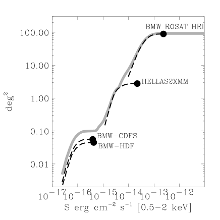
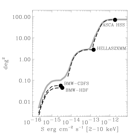
Figure 1: The sky-coverages of the the surveys described in the text are plotted. For each survey the black dot corresponds to the minimum flux for which the area of the survey is maximum: for brighter fluxes the sky coverage is flat and is not plotted. The sum is plotted with a grey line in both the soft (left panel) and hard band (right panel).

2.4 Pencil beam surveys

As pencil beam surveys we consider the two deepest look at the X–ray sky. These were provided by the Chandra 1 Ms look at the CDFS (Rosati et al. 2002) and at the Hubble Deep Field North (HDFN; Brandt et al. 2001).

The CDFS consists of eleven observations for an effective exposure time of 940 ks. We analyzed the inner $8^{\prime}$ radius image with a dedicated wavelet detection algorithm (BMW-Chandra; see Moretti et al. 2002). We detected 244 and 177 sources reaching limiting fluxes of $2.44\times 10^{-17}$ and $2.10\times 10^{-16}$ erg s^-1 cm^-2 in the soft (0.5–2 keV) and hard (2–10 keV) bands, respectively. A full account of this analysis can be found in Campana et al. (2001) and Moretti et al. (2002).

With the same detection algorithm and procedures adopted for the analysis of the CDFS we analysed the 1 Ms exposure of the HDFN. The HDFN consists of twelve observations for a total nominal exposure time of 978 ks. The data were filtered to include only the standard event grades 0, 2, 3, 4 and 6. All hot pixels and bad columns were removed. Time intervals during which the background rate is larger than $3\,\sigma$ over the quiescent level were also removed in each band separately. This results in a net exposure time of 952 ks in the soft band and 947 ks in the hard band, respectively. We removed also flickering pixels with two or more events contiguous in time (time interval of 3.2 s). The twelve observations were co-added with a pattern recognition routine to within $0.4^{\prime\prime}$ r.m.s. pointing accuracy. We restricted our analysis to the fully exposed ACIS-I area. Exposures were taken basically at two different positions separated by $6^{\prime}$. The fully exposed region thus has a rectangular shape. Within this region we also restricted to a circular region with $8^{\prime}$ radius from the barycenter of the observations for sky-coverage purposes (see below). The full sky–coverage is $\sim 0.045$ deg² ($10\%$ smaller than in the CDFS). The average background in the considered region is 0.07 (0.12) counts s^-1 per chip in the soft (hard) band and is in very good agreement with the expected values reported in the Chandra Observatory Guide. We adopted a count-rate to flux conversion factors in the 0.5–2 keV and in the 2–10 keV bands of $4.5\times 10^{-12}$ erg s^-1 cm^-2 and of $2.66\times 10^{-11}$ erg s^-1 cm^-2 respectively. These numbers were computed assuming a Galactic absorbing column of $1.6\times 10^{20}$ cm^-2 and a power law spectrum with a photon index $\Gamma=1.4$.

We run our BMW algorithm tailored for the analysis of Chandra fields, in the same way and with the same thresholds used in the analysis of the CDFS (Campana et al. 2001; Moretti et al. 2002). We detected 214 and 170 sources in the soft and hard band, respectively; 39 sources ($\sim 15\%$ of all detected sources) are revealed only in the hard band, and 83 ($\sim 33\%$) only in the soft band (Fig. 2).

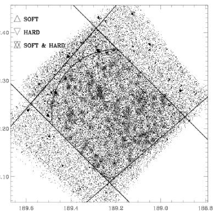
Figure 2: The BMW surveyed area of the Chandra HDF region: we restricted our analysis to a circular region of 8 arcmin radius centered on the barycenter of the maximum exposed region. The BMW source catalog from the 1Ms Chandra observation of the HDF is the only survey we use in this work not yet published.

As for the CDFS we carried out extensive simulations (400 fields per band) to assess with very good accuracy the sky coverage. Moreover, we corrected for the Eddington bias following the approach by Vikhlinin et al. (1995) as described in Moretti et al. (2002). The Eddington bias starts affecting the HDFN data at a level of $\sim 20$ counts in the soft band ($\sim 9\times 10^{-17}\rm\ erg\,s^{-1}\rm\ cm^{-2}$) and $\sim 30$ counts in the hard band ($\sim 8\times 10^{-16}\rm\ erg\,s^{-1}\rm\ cm^{-2}$). Our simulations show that we are able to recover the number source distribution down to 5 (7) corrected counts in the inner core of the image, declining to 9 (11) corrected counts in the outskirts for the soft (hard) band. These counts gives a flux limit in the inner region of $3.51\times 10^{-17}$ erg s^-1 cm^-2 and $2.29\times 10^{-16}$ erg s^-1 cm^-2 in the soft and hard band, respectively. The sky coverage of these surveys are shown in Fig. 1.

In order to evaluate the possible cosmic variance between the two deep fields we compared the faint end of the two flux distributions. In both cases we found that, excluding the bright sources ($>5\times 10^{-15}\rm\ erg\,s^{-1}\rm\ cm^{-2}$), the values of the analytical fits (slope and normalization) realtive to the two fields are compatible at $1\sigma$ level to each other and with the values relative to the fit of the entire sample (see below).

3 Contribution of very bright sources to the background

The surveys under consideration lack of a proper covering at the brightest flux levels: in fact most of the X–ray brightest sources are the target of the observation and are excluded from serendipitous catalogs. For this reason in these surveys we cut the source flux distributions at $10^{-11}$ ($8\times 10^{-12}$) erg cm^-2 s^-1 in the soft (hard) band. Note that even if the number of these bright sources is relatively small (less than a few hundred sources on the whole sky), their contribution to the CXB is not negligible.

To overcome this problem, in the case of the soft band, we took advantage of the ROSAT Bright Survey (RBS, Schwope et al. 2000) that contains all sources of the ROSAT All Sky Survey (RASS) sources with count rate larger than 0.5 c s^-1. There are 93 high galactic latitute extragalactic sources brighter than $10^{-11}$ erg cm^-2 s^-1 which provide a density flux of $F_{S11}=1.45\times 10^{-13}$ erg cm ^-2 s^-1 deg^-2 in the 1–2 keV energy band or $3.2\%$ of the CXB (see below).

For the hard band we considered the HEAO-1 A2 extragalactic survey which is complete down to $3.1\times 10^{-11}$ erg cm^-2 s^-1 (Piccinotti et al. 1982). The total flux of the 66 sources amounts to $F_{H11}=4.28\times 10^{-13}$ erg cm^-2 s^-1 deg^-2 or $2.1\%$ of the CXB (see below). To include the small intermediate interval ($8.0\times 10^{-12}$ and $3.1\times 10^{-11}$ erg cm^-2 s^-1) not covered by the hard X–ray surveys we will extrapolate the Log N–Log S relation.

4 Contribution from extended sources

A significant fraction of the CXB is made up by the thermal bremsstrahlung emission from clusters of galaxies. In the soft band (1–2 keV) this fraction is estimated at a level of $\sim 6\%$ from direct measurments of the cluster Log N–Log S (Rosati et al. 1998, 2002). In the hard band there is not a precise determination, but this can be estimated to be at a level of $\sim 5\%$ from the Log N–Log S (e.g. Gilli et al. 1999, derived from Ebeling et al. 1997). So far, in the building of the general source catalog, no selection have been made among different kind of sources. Clusters of galaxies are included in our catalog as well the other cosmological sources (AGN and QSO).

In the construction of the Log N–Log S, if we treat clusters of galaxies in the same way as point-like sources, we then introduce flaws. First, the X–ray spectrum of a cluster of galaxies is different from the other point-like sources and therefore the conversion factor changes. More importantly, clusters of galaxies, having extended emission, have different sky–coverages with respect to point–like sources (for a given instrument, at the same flux, in general, a point–like source is more easily detected than an extended one). Thus, if we use the point-like sky coverage for all sources, we underestimate the level of the integrated flux because we underestimate the statistical weight of the extended sources. Clearly, this difference is particulary pronunced in the case of surveys based on high spatial resolution instruments (Chandra, ROSAT-HRI, XMM–Newton), whereas it is neglegible for the ASCA-HSS survey.

To evaluate the contribution of the extended sources to the CXB we can use only our BMW surveys (i.e. ROSAT-HRI and Chandra), for which we have an extension flag. In the BMW-HRI catalog we have 199 extended sources, which correspond to $5\%$ of the sources of the catalog. An appropriate sky coverage for the extended sources of the BMW-HRI catalog has been derived from extensive Montecarlo simulations described in Moretti et al. (2003). We estimate that the contribution of these clusters treated as extended and not point–like, increases, going from $3.5\%$ to $\sim 6\%$ of the total 1-2 keV CXB flux (see next Section) which is in very good agreement with Rosati et al. (2002). At lower fluxes we estimate an extra contribution from clusters in the HELLAS2XMM survey of $\sim 1\%$. Being this just an estimate we include it in the error budget.

In the hard band, the arcmin angular resolution of ASCA makes any correction due to the presence of extended sources negligible. We estimate, from preliminary classification of HSS sources (Della Ceca et al. 2001), that the total correction due to the changing in the conversion factor is $<1\%$ and we include it in the calculation of the uncertainties. At fainter fluxes, the contribution of extended sources in the hard band of the HELLAS2XMM survey is estimated to be $<1\%$ which is again included in the error budget.

Figure 3: Left panel: soft CXB (1–2 keV) measurements spaced in time along with their $68\%$ error bars; the constant line represents the best fit to all these measurements ($\chi^{2}_{\rm red}=0.9$). CXB values (left to right) are from Gorenstein et al. (1969); Garmire et al. (1992); Gendrau et al. (1995); Georgantopoulos et al. (1996); Chen et al. (1997); Miyaji et al. (1998); Parmar et al. (1999); Vecchi et al. (1999); Kuntz et al. (2001); Lumb et al. (2002). Right panel: hard CXB (2–10 keV) measurements spaced in time along with their $68\%$ error bars; the constant line represents the best fit to all these measurements ($\chi^{2}_{\rm red}=1.3$). CXB values (left to right) are from Gorenstein et al. (1969); Palmieri et al. (1971); Marshall et al. (1980); McCammon et al. (1983); Gendrau et al. (1995); Chen et al. (1997); Miyaji et al. (1998); Ueda et al. (1999); Vecchi et al. (1999); Lumb et al. (2002); Kushino et al. (2002).

5 X–ray background level

Measuring the CXB flux has been one of the most challanging tasks of X–ray astronomy. Several measurements have been carried out with rockets and satellites. Barcons et al. (2000) found that, while the differences in the measurments among different studies using different data from the same instrument can be ascribed to the cosmic variance, systematic differences remain among different missions. Following Gilli (2002), we made a bibliographic search selecting ten and eleven measurements in the soft (1–2 keV) and hard (2–10 keV) energy bands, respectively. We compute $68\%$ errors estimates on the flux adding the contribution of the bright sources when they have been excluded from the analysis (Hasinger 1996). Our results are reported in Fig. 3. A fit with a constant provides a good representation in terms of reduced $\chi^{2}$. In the soft band (1–2 keV) we derive a value of $(4.54\pm 0.21)\times 10^{-12}$ erg s^-1 cm^-2 deg^-2 ($90\%$ confidence level) with a $\chi^{2}_{\rm red}=0.9$. Assuming the average value for the slope of the spectrum ($\Gamma=1.4$, Rosati et al. 2002) this value correspond to $(7.53\pm 0.35)\times 10^{-12}$ erg s^-1 cm^-2 deg^-2 in the 0.5–2 keV band. In the hard band we obtain $(2.02\pm 0.11)\times 10^{-11}$ erg s^-1 cm^-2 deg^-2 with a $\chi^{2}_{\rm red}=1.3$ ($32\%$ null hypothesis probability). These values, in both band, are in excellent agreement with the CXB intensity value reported in Barcons et al. (2000). Thus, despite the variability reported in the literature our fit indicates that the different estimates of the soft and hard CXB are consistent each other in a statistical sense.

6 Conversion factors and cross–calibrations

The CXB is the result of the integrated emission of a mix of different sources, mainly unabsorbed and absorbed AGNs. The resulting spectrum in the energy range of our interest can be modelled with a power law with $Gamma\sim 1.4$, which is very different from the spectrum slope of the typical sources which make it: this is the so called spectral paradox and was explained for the first time by Setti & Woltijer (1979). An important point in our work is the choice of the spectrum for converting counts to fluxes. In all the surveys we used to build the catalog a single spectrum slope $\Gamma$ has been assumed; these values, reported in Table 1, have been chosen to match the expected average spectrum of the sources: they change significantly from survey to survey passing from $\Gamma=2$ in the BMW to $\Gamma=1.4$ in the Chandra deep surveys (Table 1). Cowie et al. (2002) in the Chandra deep field analysis adopted $\Gamma=1.2$ pointing out that the average spectra at very faint fluxes is harder than that of the CXB. In different ranges of flux the slope of the average spectrum revealed from the staked spectrum analysis of the sources change passing from steeper values to shallower values with the flux lowering (e.g. Tozzi 2001). In the case of our work we have two requirments: the first is to make all the sample homogeneous and the second is that because we use a very large flux range we have to account for the changing of the CXB spectrum as the flux lowers. Our approach is the following: using literature data we attributed to each source a different spectral slope as a function of its flux. For this reason we collected spectral indexes from bright to faint ends from several surveys (soft: Vikhlinin et al. 1995; Brandt et al. 2001; hard: Della Ceca et al. 1999; Rosati et al. 2002). These power law indexes have been fitted (with a Fermi function) as a function of the X–ray flux (in the soft and hard band separately). Then we checked that the integrated spectrum is consistent with the expected one: in both bands we considered the integrated spectrum built summing the contribution of each source weighted by the sky coverage and we found that they are both perfectly consistent with the expected one ($\Gamma~{}1.4$), having taken into account also the contribution of the clusters. The flux of each source has then been corrected for the ratio of the nominal conversion factor used in the survey and the one recalculated by us, with the interpolated power law index at the appropriate column density. Flux corrections for single sources are on average $\sim 5\%$ ($\sim 7\%$ in the hard band) and always less than $17\%$.

Absolute cross–calibration between XMM–Newton and Chandra have not been yet well explored. Lumb et al. (2001) found that Chandra fluxes are sistematically $10\%$ higher than XMM ones, once the differences of the detection procedures have been took into account, without any trend with spectral slope, off–axis angle or brightness. In order to evaluate how the different normalization of the different instruments could affect our calculation, we artificially increased and reduced the flux of the single survey (one by one) by a $10\%$ factor (modifying the corresponding sky–coverage). We found that we have typical differences of $2\%$ of the total CXB (and never larger than $3\%$).

7 Global Log N–Log S

The cumulative flux distribution (Log N–Log S) at each flux $S$ is the number of all sources brighter than $S$ weighted by the corresponding sky–coverage:

$$N(S)=\sum_{S_{i}>S}\frac{1}{\Omega_{\rm tot}(S_{i})~{}}$$ (1)

here the sky–coverage $\Omega_{\rm tot}$ is the sum of the contributions of all surveys in each band (Fig. 1). Given the large flux interval spanned, we consider as analytical form of the integral source flux distribution two power laws with index $\alpha_{\rm 1,s(h)}$ and $\alpha_{\rm 2,s(h)}$ for the bright and faint part respectively, joining without discontinuites at the flux $S_{\rm 0,s(h)}$:

$$N(>S)=N_{S(H)}\,\Bigl{[}{{(2\times 10^{-15})^{\alpha_{1,s(h)}}}\over{S^{\alpha_{1,s(h)}}+S_{\rm 0,\,s}^{\alpha_{1,s(h)}-\alpha_{2,s(h)}}\,S^{\alpha_{2,s(h)}}}}\Bigr{]}\ {\rm cgs}.$$ (2)

To fit the data we applied a maximum–likelihood algorithm to the differential flux distribution corrected by the sky coverage

$$\frac{dN}{dS}\times\Omega(S)\ .$$ (3)

Once we obtain the analytical form of the flux distribution we can calculate the total contribution of sources, $F_{\rm sou}$, to the CXB by integrating the quantity

$$F_{\rm sou}=\int_{S_{\rm min}}^{S_{\rm max}}\Big{(}\frac{dN}{dS}\Big{)}\times S~{}dS$$ (4)

with $S_{\rm min}$ and $S_{\rm max}$ as the boundary fluxes of our interval of interest.

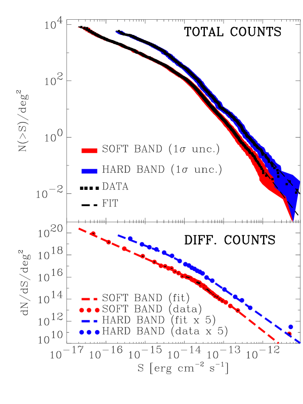
Figure 4: In the upper panel the Log N–Log S(integral) curves of our composite catalog in both soft and hard band are shown: in both cases we obtained an excellent fit with two smoothly joined power laws (see text). In the lower panel we plot the differential distributions: the data are grouped to have a minimum of 100 (50) measures in each bin in the soft (hard) band. The hard band counts are multiplied by 5 for clarity of the plot. Due to the very large y-axis range the error bars are not visible in the graph: they are approximately 10$\%$ and 15$\%$ respectively.

7.1 Soft energy band

The three source distributions (BMW-Chandra, XMM2HELLAS and BMW-HRI) containing point and extended sources, cover with good signal to noise ratio the flux range $2.4\times 10^{-17}-10^{-11}$ erg cm^-2 s^-1. We found a good fit with $\alpha_{\rm 1,s}=1.82^{+0.07}_{-0.09}$, $\alpha_{\rm 2,s}=0.60^{+0.02}_{-0.03}$, $S_{\rm 0,s}=(1.48^{+0.27}_{-0.31})\times 10^{-14}$ erg cm^-2 s^-1 and $N_{S}=6150^{+1800}_{-1650}$ (errors at $68\%$ confidence for the four parameters i.e. $\Delta\chi^{2}=4.72$, see Fig. 4).

In order to calculate the reduced $\chi^{2}$ we adaptively binned the data to contain 50 sources per bin: we obtain $\chi^{2}_{red}=1.4$ with 87 degrees of freedom (null hypothesis probability $\sim 1\%$). From the residual analysis we find that the largest scatter between data and fit is in the knee region, where the two power laws join. This has to be ascribed to the choice of the analitycal function rather than a mismatch between different surveys: a function with one more parameter could improve the reduced $\chi^{2}$ value.

As expected, the slope of the bright part is consistent with the previous determinations. Panzera et al. (2002) has already shown that the BMW HRI log N–log S is in excellent agreement with the bright part of the distribution reported by Hasinger et al. (1998). Here, using also the HELLAS2XMM data, we find a slightly steeper value for the bright slope (consistent at $1\sigma$ level): $1.68\pm 0.27$ vs. $1.82\pm 0.09$. In the faint end we find good agreement with Rosati et al. (2002), Brandt et al. (2001) and Mushotzky et al. (2000) who report $0.60\pm 0.13$, $0.6\pm 0.1$ and $0.7\pm 0.2$, respectively.

The fitted Log N–Log S distribution gives in the 0.5–2.0 keV band an integrated flux $F_{\rm sou}=6.85^{+0.28}_{-0.23}\times 10^{-12}$ erg s^-1 cm^-2 deg^-2. This corresponds to $91.0^{+3.8}_{-3.1}\%$ of the corresponding CXB value. Adding the contribution at brighter fluxes (see Section 3) and taking into account the uncertainties in the correction for XMM2HELLAS clusters of galaxies (Section 4) and the uncertainties in the conversion factor and in the cross–calibration (Section 6) we end up with $F_{S11}+F_{\rm sou}=94.3_{-6.7}^{+7.0}\%$ of resolved CXB (see Fig. 5).

7.2 Hard energy band

We fit with the same functional form of equation (4) the hard Log N–Log S distribution.

The flux interval with good signal to noise ratio is $2.1\times 10^{-16}-8.0\times 10^{-12}$ erg cm^-2 s^-1. We found a good fit with $\alpha_{\rm 1,h}=1.57^{+0.10}_{-0.08}$, $\alpha_{\rm 2,h}=0.44^{+0.12}_{-0.13}$, $S_{\rm 0,h}=(4.5^{+3.7}_{-1.7})\times 10^{-15}$ erg cm^-2 s^-1 and $N_{H}=5300^{+2850}_{-1400}$ (errors at $68\%$ confidence as before, see Fig. 4).

In order to calculate the reduced $\chi^{2}$ we adaptively binned the data to contain 25 sources per bin: we obtain $\chi^{2}_{red}=0.93$ with 38 degrees of freedom (null hypothesis probability $\sim 60\%$). This assures us of the goodness of the fit and the effective possibility to smoothly match data from different surveys performed with different instruments also in the hard band.

In the bright part, after summing the HELLAS2XMM data to the ASCA–HSS data, we find a slightly steeper value (still consistent at $1\sigma$ level) with respect to the value reported in Cagnoni et al. (1998) and the one based on BeppoSAX (Giommi, Perri & Fiore 2000). Our determination of the faint hard slope ($\alpha_{\rm 2,h}=0.44^{+0.12}_{-0.13}$) is flatter and only marginally consistent with Rosati et al. (2002) (0.61$\pm 0.10$), Cowie et al. (2002) (0.63$\pm 0.05$) and Mushotzky et al. (2000) (1.05$\pm 0.35$ using a single power law). This is probably correlated to the different position that we estimate for the knee of the double power law ($S_{\rm 0,h}=(4.5^{+3.7}_{-1.7})\times 10^{-15}$ erg cm^-2 s^-1) which is fainter both than the value reported in Cowie et al. (2002) ($1.2\times 10^{-14}$) erg cm^-2 s^-1 and the value reported in Rosati et al. (2002) ($\sim 8\times 10^{-15}$) erg cm^-2 s^-1.

Our fitted Log N–Log S distribution gives an integrated flux $F_{\rm sou}=1.75^{+0.11}_{-0.10}\times 10^{-11}$ erg s^-1 cm^-2 deg^-2. This accounts for $86.7^{+5.5}_{-5.9}\%$ of the CXB (the $1\,\sigma$ uncertainties interval are reported). Adding the contribution of brighter sources (Section 3) and taking into account the uncertainties in the conversion factor and in the cross–calibrations (Section 6) and the uncertainty of the contribution of extended sources (Section 4) we obtain a resolved fraction of $F_{H11}+F_{\rm sou}=88.8_{-6.6}^{+7.8}\%$ (see Fig. 5).

8 Summary and conclusions

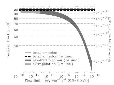
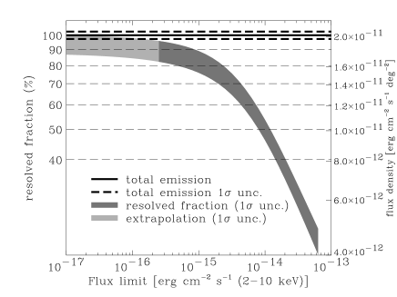
Figure 5: The fraction of resolved background as function of the flux limit in the soft 0.5–2 keV (upper) and hard 2–10 keV (lower) energy bands. On the right axis of each plot the absolute value of the flux density is reported in the 0.5–2 and 2–10 keV

While the high spatial resolution and positional accuracy of the Chandra satellite allow us to investigate the faintest sources which make up the CXB and to identify most of the detected photons as emission from discrete sources, the fluctuations in the source number counts among the different Chandra deep fields reach a $30\%$ level for the bright sources (see Setion 2.4 and Tozzi 2001). These fluctuations correspond to very high uncertainties in the calculation of the fraction of the total CXB that we can resolve in discrete sources. In order to improve the statistics we matched data from different surveys. The resulting composite catalog allowed us to draw with good statistics the Log N–Log S curve over the maximum possible flux range with the data currently available: [$2.44\times 10^{-17}-1.00\times 10^{-11}$] erg s^-1 cm^-2 in the soft band and [$2.10\times 10^{-16}-7.79\times 10^{-12}]$ in the hard band (see Fig. 4). Moreover, we derived a reliable value of the measure of the total CXB by means of a critical review of the literature values. We calculated that in the range of our composite catalogs the detected sources make up $94\%$ and $89\%$ of the total soft and hard CXB emission, respectively. We obtained a good fit of the flux distribution in both bands with two smoothly joined power laws: this demonstrates that we can use data obtained with different instruments in a coherent manner.

If we extrapolate the analytical form of the Log N–Log S distribution beyond the flux limit of our catalog in the soft band we find that the integrated flux from discrete sources at $\sim 3\times 10^{-18}$ erg s^-1 cm^-2 (a factor 10 lower than the catalog limit) is $96\%$ of the total CXB and it is consistent with its full value at $1\sigma$ level (comparing the best value for the integrated flux from discrete sources with the CXB $1\sigma$ uncertainty).

In the hard band, extending again to lower fluxes the Log N–Log S distribution we can make up only $93\%$ of the total CXB, at most. This is only marginally consistent with the CXB total value. The small contribution of the faint sources is due to the fact that the Log N–Log S distribution converges less than logarithmically (Fig. 5). This leaves space to the presence of a class of very faint hard sources only poorly detected in the 2–10 keV band within the actual limits or even to diffuse emission. This class of sources could consist of heavily absorbed AGN which are expected to provide higher contributions to the X–ray counts at higher energies. A possible indication of the existence of this population could be the steepeer source counts found in the very hard band (5–10 keV), as reported in Rosati et al. (2002). According to the model by Franceschini et al. (2002, see also Gandhi & Fabian 2002), which is based on IR statistics, in the 2–10 keV band the contribution of obscured AGN would become dominant at $\sim 10^{-15}$ erg s^-1 cm^-2. A qualitative study of this model allow us to estimate that the existence of such a class of sources would result in a steepening of the hard Log N–Log S below $\sim 4\times 10^{-16}$ erg s^-1 cm^-2 which could fill the remaining fraction of unresolved CXB. The approximate extra–contribution is estimated to be about $\sim 10^{-12}$ erg s^-1 cm^-2deg^-2 (5$\%$ of the total) in the range between $4\times 10^{-17}$ and $2\times 10^{-16}$ erg s^-1 cm^-2. Actually our data could neither confirm nor reject this eventual steepening being very close to the limit of our catalog. Another possibility recently put forward is represented by X–ray emission from star-forming galaxies that can make up to $11\%$ of the hard CXB by extrapolating the radio counts down to 1 Jy or $10^{-18}$ erg s^-1 cm^-2 in the soft X-ray band (Ranalli et al. 2002). In this contest the analysis of the HDF Chandra deeper observation (2Ms) and the XMM–Newton surveys will be crucial.

References

- (1) Akiyama, M., et al. 2000, ApJ, 532, 700.
- (2) Baldi, A., Molendi, S., Comastri, A., Fiore, F., Matt, G., Vignali, C. 2002, ApJ, 564, 190.
- (3) Barcons, X., Mateos, S, Ceballos, M.T. 2000, MNRAS, 316, L13.
- (4) Barger, A.J., Cowie, L.L., Mushotzky, R.F., Richards, E.A. 2001, AJ, 121, 662.
- (5) Brandt, W.N., et al. 2001, AJ, 122, 2810.
- (6) Cagnoni, I., della Ceca, R., Maccacaro, T. 1998, ApJ, 493, 54.
- (7) Campana, S., Lazzati, D., Panzera, M.R., Tagliaferri, G. 1999, ApJ, 524, 423.
- (8) Campana, S., Moretti, A., Lazzati, D., Tagliaferri, G. 2001, ApJ, 560, L19.
- (9) Chen, L., Fabian, A.C., Gendreau, K.C. 1997, MNRAS, 285, 449.
- (10) Chiappetti, L., Cusumano, G., del Sordo, S., Maccarone, M.C., Mineo, T., Molendi, S. 1998, in The Active X-ray Sky: Results from BeppoSAX and RXTE. eds. L. Scarsi, H. Bradt, P. Giommi, F. Fiore. (Elsevier, Amsterdam), 610.
- (11) Cowie, L. L.; Garmire, G. P.; Bautz, M. W.; Barger, A. J.; Brandt, W. N.; Hornschemeier, A. E. 2002 AJ, 123, 2197.
- (12) della Ceca, R., Castelli, G., Braito, V., Cagnoni, I., Maccacaro, T., 1999 ApJ, 524, 674.
- (13) della Ceca, R., Braito, V., Cagnoni, I., Maccacaro, T. 2001, Mem. SAIt, 72, 841.
- (14) Ebeling, H.; Edge, A. C.; Fabian, A. C.; Allen, S. W.; Crawford, C. S.; Boehringer, H. 1997, ApJ, 479, L101.
- (15) Fiore, F., et al. 1999, MNRAS, 306, L55.
- (16) Franceschini, A.; Braito, V.; Fadda, D. 2002 MNRAS, 335, L51.
- (17) Gandhi, P.; Fabian, A.C. 2002, MNRAS in press (astro-ph/0211129).
- (18) Garmire, G. P.; Nousek, J. A.; Apparao, K. M. V.; Burrows, D. N.; Fink, R. L.; Kraft, R. P. 1992, ApJ, 399, 694.
- (19) Gendreau, K.C., et al. 1995, PASJ, 47, L5.
- (20) Georgantopoulos, I., Stewart, G. C., Shanks, T., Boyle, B. J., Griffiths, R. E., 1996, MNRAS, 280, 276.
- (21) Giacconi R., Gursky H., Paolini F. R., Rossi B. B., 1962, Phys. Rev. Lett., 9, 439.
- (22) Giacconi, R., et al. 2002, ApJS, 139, 369.
- (23) Gilli, R.; Risaliti, G.; Salvati, M. 1999, A&A, 347, 424.
- (24) Gilli, R. 2002, proceedings from AGN5:Inflows, Outflows and Reprocessing around black holes (http://www.unico.it/ilaria/AGN5/proceedings.html).
- (25) Giommi, P., Perri, M., & Fiore, F. 2000, A&A, 362, 799.
- (26) Gorenstein, P., Kellogg, E. M., Gursky, H. 1969 ApJ, 156, 315.
- (27) Hasinger, G., 1996, proceedings from IAU Symposium 168. M. C. Kafatos, and Y. Kondo, Kluwer Academic Publishers, 245.
- (28) Hasinger, G., Burg, R., Giacconi, R., Schmidt, M., Trümper, J., Zamorani, G. 1998, A&A, 329, 482.
- (29) Hasinger, G., et al. 2001, A&A, 365, L45.
- (30) Hornschemeier, A.E., et al. 2000, ApJ, 541, 49.
- (31) Hornschemeier, A.E., et al. 2001, ApJ, 554, 742.
- (32) Kuntz, K.D., Snowden, S.L., Mushotzky, R.F. 2001, ApJ, 548, L119.
- (33) Kushino, A.; Ishisaki, Y.,Morita, U., Yamasaki, N. Y., Ishida, M., Ohashi, T. Ueda, Y. 2002, PASJ, 54, 327.
- (34) Lazzati, D., Campana, S., Rosati, P., Panzera, M.R., Tagliaferri, G. 1999, ApJ, 524, 414.
- (35) Lehmann, I., et al. 2001, A&A, 371, 833.
- (36) Lumb, D. H., Warwick, R. S.; Page, M., De Luca, A. 2002, A&A, 389, L93.
- (37) Lumb, D. H., Guainazzi, M., Gondoin, P., 2001, A&A, 376, 387.
- (38) Mather, J.C. et al. 1990, ApJ, 354, L37.
- (39) Marshall, F.E., et al. 1980, ApJ, 235, 4.
- (40) McCammon, D., Burrows, D.N., Sanders, W.T., Kraushaar, W.L. 1983, ApJ, 269, 107.
- (41) Miyaji, T., Ishisaki, Y., Ogasaka, Y., Ueda, Y., Freyberg, M. J., Hasinger, G., Tanaka, Y., 1998, A&A, 334, L13.
- (42) Miyaji, T., Griffiths, R. E. 2002, ApJ, 564, L5.
- (43) Moretti, A., Lazzati, D., Campana, S., Tagliaferri, G. 2002, ApJ, 570, 502.
- (44) Moretti, A. et al., 2003 in preparation.
- (45) Mushotzky, R.F., Cowie, L.L., Barger, A.J., Arnaud, K.A. 2000, Nat, 404, 459.
- (46) Palmieri, T. M.; Burginyon, G. A.; Grader, R. J.; Hill, R. W.; Seward, F. D.; Stoering, J. P. 1971, ApJ, 169, 33.
- (47) Panzera, M. R., Campana, S., Covino, S., Lazzati, D., Mignani, R., Moretti, A., Tagliaferri, G., 2002, A&A in press (astro-ph/0211201).
- (48) Parmar, A. N., Guainazzi, M., Oosterbroek, T., Orr, A., Favata, F., Lumb, D., Malizia, A., 1999, A&A, 345, 611.
- (49) Piccinotti, G.; Mushotzky, R. F.; Boldt, E. A.; Holt, S. S.; Marshall, F. E.; Serlemitsos, P. J.; Shafer, R. A. 1982 ApJ, 253, 485.
- (50) Ranalli, P.; Comastri, A.; Setti, G. 2002, A&A in press (astro-ph/0211304).
- (51) Rosati, P., della Ceca, R., Burg, R., Norman, C., Giacconi, R. 1995, ApJ, 445, L11.
- (52) Rosati, P., Della Ceca, R., Norman, C., Giacconi R., 1998, ApJ, 492, L21.
- (53) Rosati, P., et al. 2002, ApJ, 566, 667.
- (54) Schmidt, M., et al. 1998, A&A, 329, 495.
- (55) Schwope, A., et al. 2000 AN, 321, 1.
- (56) Setti, G., Woltjer, L. 1989, A&A, 224, L21.
- (57) Tozzi, P., et al. 2001, ApJ, 562, 42.
- (58) Ueda, Y., et al. 1999, ApJ, 518, 656.
- (59) Vecchi, A., Molendi, S., Guainazzi, M., Fiore, F., Parmar, A.N. 1999, A&A, 349, L73.
- (60) Vikhlinin, A., Forman, W., Jones, C. Murray, S. 1995, ApJ, 451, 542.