Are the Faraday Rotating Magnetic Fields Local to Intracluster Radio Galaxies?

Abstract

We investigate the origin of the high Faraday rotation measures (RMs) found for polarized radio galaxies in clusters. The two most likely origins are, magnetic fields local to the source, or magnetic fields located in the foreground intra-cluster medium (ICM). The latter is identified as the null hypothesis. Rudnick & Blundell (2003) have recently suggested that the presence of magnetic fields local to the source may be revealed in correlations of the position angles (PAs) of the source intrinsic linear polarization and the RMs. We investigate the claim of Rudnick & Blundell to have found a relationship between the intrinsic PA₀ of the radio source PKS 1246-410 and its RM, by testing the clustering strength of the PA₀-RM scatter plot. We show that the claimed relationship is an artifact of an improperly performed null-experiment. We describe a gradient alignment statistic aimed at finding correlations between PA₀ and RM maps. This statistic does not require any null-experiment since it gives a unique (zero) result in the case of uncorrelated maps. We apply it to a number of extended radio sources in galaxy clusters (PKS 1246-410, Cygnus A, Hydra A, and 3C465). In no case is a significant large-scale alignment of PA₀ and RM maps detected. We find significant small-scale co-alignment in all cases, but we are able to fully identify this with map making artifacts through a suitable statistical test. We conclude that there is presently no existing evidence for Faraday rotation local to radio lobes. Given the existing independent pieces of evidence, we favor the null hypothesis that the observed Faraday screens are produced by intracluster magnetic fields.

1 Introduction

A detailed summary of the observational evidence for the presence of magnetic fields embedded within the thermal gas in clusters of galaxies is presented in two recent review papers (Carilli & Taylor 2002, and Widrow 2002) and is only briefly summarized here.

Magnetic fields in galaxy clusters are known to exist due to the detection of diffuse cluster wide synchrotron emission (Willson 1970) in a number of clusters. This emission is not associated with individual galaxies in the cluster and is observationally classified as halo or relic emission (Feretti 1999). Although initially thought to be relatively rare objects, recent surveys have significantly increased the number of radio halos and relics (Giovannini, Tordi, & Feretti 1999; Giovannini & Feretti 2000; Kempner & Sarazin 2001; Bacchi et al. 2003). The presence of this diffuse synchrotron emission reveals the widespread distribution of magnetic fields within the intracluster medium (ICM) in these clusters. Equipartition assumptions provide minimum energy magnetic field estimates in radio halos of 0.1 - 1 $\mu$G (Feretti 1999; Bacchi et al. 2003) and 0.4 - 2.7 $\mu$G in radio relics (Enßlin et al. 1998).

Estimates of volume averaged intracluster magnetic field strengths can be obtained by comparing the synchrotron and inverse Compton emission (e.g., Harris & Grindlay 1979, Rephaeli et al. 1987). The same relativistic particle population which produces the diffuse synchrotron emission is expected to up-scatter the ambient photon field in the ICM to produce inverse Compton X-rays. Typical estimates yield a volume-averaged intracluster magnetic field in the range of 0.2 - 1 $\mu$G (see e.g. Carilli & Taylor 2002 and references therein). We emphasize that inverse Compton based estimates have to be regarded as lower limits.

Faraday rotation measure (RM) studies of extended radio sources embedded in clusters probe the magnetic field component integrated along the line-of-sight, weighted by the plasma electron density. Faraday rotation is the rotation of the position angle (PA) of the plane of linear polarization of radio waves, which traverse a magnetized plasma. The RM is the proportionality constant of this $\lambda^{2}$-dependent effect: ${\rm PA}(\lambda)={\rm PA}_{0}+\lambda^{2}\,{\rm RM}$, where PA₀ is the source intrinsic PA, only directly observable at shortest wavelength. The RM and PA₀ can be obtained by multi-frequency measurements of a polarized radio source.

Carilli & Taylor (2002) review the generally large RM values obtained from extended radio sources embedded in clusters, and summarize the evidence that indicates that the observed RM of embedded sources are indeed probing a foreground ICM, with conservative estimates of magnetic field strengths between a few $\mu$G and 10s of $\mu$G. Similar magnetic field strengths are determined from statistical RM studies by Kim, Tribble & Kronberg (1991), and Clarke, Kronberg & Böhringer (2001).

Finally, the asymmetric depolarization of double radio lobes embedded in galaxy clusters can be understood as resulting from a difference in the Faraday depth of the two lobes (Laing 1988; Garrington et al. 1988) which strongly supports the association of RMs with ICM magnetic fields. We note that such a difference in Faraday depth might also be explained by local effects near the source, if there is a difference in the mixing layers of the magnetized radio plasma with the dense environmental gas between the radio lobe head side and the back-flow side of an FR II radio galaxy. In contrast, this scenario would have difficulties to explain the observed strong RM and depolarization asymmetry of FR I radio galaxies like Hydra A (Taylor & Perley 1993), which are not believed to have back-flows. However, this discussion shows that the association of the RM with the intra-cluster medium – in the following regarded as the null hypothesis – is not unambiguous, since it could also be produced in a magnetized plasma skin or mixing layer of the observed radio galaxy (Bicknell et al. 1990). For that reason Rudnick & Blundell (2003, hereafter RB) used Faraday rotation measure observations of PKS 1246-410 by Taylor, Fabian & Allen (2002) in an attempt to estimate the fraction of the measured RM signal which is local to the radio source. If most of the RM signal is local to the radio source then the derived ICM magnetic field strength should be significantly lower than if all of the RM originates in the ICM.

In the following we examine RB’s claim for evidence of source-local magnetic fields. We do this first through a general argument (Sect. 2) followed by an illustrative numerical example (Sect. 3). Then, in order to have an unbiased tool to measure cross correlations of RM and PA maps, we specify the mathematical requirements of a suitable statistic (Sect. 4), and construct a gradient alignment statistic which meets our quality criteria (Sect. 5). This statistic is also sensitive to correlated noise resulting from the map making imperfections (Appendix B). We therefore design a gradient vector product statistic, which is only sensitive to such imperfections, in order to separate spurious signals from any astrophysical signal (Sect. 6). Application of our approach to several datasets (PKS 1246-410, Cygnus A, Hydra A, and 3C465) does not reveal any evidence for source-local magnetic fields (Sect. 7). We conclude (Sect. 8) that the null hypothesis that the RMs are connected to the ICM is not only consistent with, but also strongly favored by present data. The basic assumption for Faraday rotation based ICM magnetic field estimates of RM being mostly generated by the ICM magnetic fields seems therefore to be valid.

2 PA₀-RM scatter plots

If the Faraday rotation observed in cluster radio galaxies is produced by a mixing layer between the radio lobe and the ICM gas then it is possible that the magnetic structures within the Faraday screen are somehow related to the magnetic field orientation within the radio lobes. In such a case, co-spatial structures in RM and PA₀ maps are possible since both quantities contain geometrical information about the source local magnetic field geometry: The PA₀ gives the plane-of-the-sky direction perpendicular to the sky-projected magnetic field within the radio lobe, and the RM the line-of-sight component of the magnetic field within the Faraday rotating medium.

The idea of RB is to test the above scenario by searching for the expected co-spatial structures in the PA₀ and RM maps of the radio galaxy PKS 1246-410. One difficulty with such an analysis is that no direct correlation between the PA₀ and RM values can be expected even for co-spatial structures, since there is no generic reference point for PA₀s. Therefore RB analyzed the PA₀-RM scatter plot generated by plotting for each map pixel the PA₀ and the RM value in the same diagram. They argue that local co-alignment of PA₀ and RM values should lead to a strongly clustered point distribution in the scatter plot. Since statistically independent PA₀ and RM maps may also produce such clusters they perform a null-experiment. They generate synthetic RM maps, which have the same power-spectrum as the observed RM map, but random phases. With these simulated maps they repeat their analysis and find much less clustering in the scatter plot. From this they conclude that there is a strong co-alignment in the PA₀-RM maps of PKS 1246-410, and therefore most of the RM should be local to the radio source. In order to give further support to their claim, they report a number of regions in a larger sample of radio galaxy maps where they see corresponding structures in the RM and PA₀ maps.

This latter finding is statistically very questionable, since within any two large datasets the human eye often finds apparent correlations within some sub-regions, even if the two datasets are uncorrelated. Furthermore, observed RM and PA₀ always carry correlated noise, as recognized by RB and analytically demonstrated in Appendix B, since they are generated from the same set of PA maps. In the worst case the noise produces step-function like artifacts at the same location in RM and PA₀ maps. We note that correlated steps are present within the aforementioned regions of RM and PA₀ maps and give – at least to our eyes – the dominant contribution to the PA₀-RM correlation impression reported by RB.

However, the claim of a statistical detection of a PA₀-RM correlation can be rigorously investigated. The null-experiment applied by RB is designed to have the same two-point autocorrelation function as the observational data, but higher order correlations are neglected by the random phase realization. Unfortunately, the chosen statistic is very sensitive to such higher order correlations. Any clustering in the PA₀-RM scatter plot is caused by having patches of nearly constant values in the PA₀ and RM maps. The appearance of patches requires special relations of the Fourier phases, or – equivalently – non-trivial higher order correlation functions to be specified.

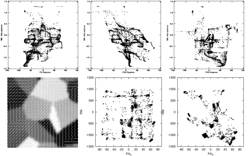
Figure 1: Upper left panel: Uncorrected PA-RM scatter plot of PKS 1246-410 (similar to Figure 4 of RB). The underlying maps were smoothed by a median weight filter in the same way as RB smoothed the data in order to amplify the clustering. Upper middle panel: Similar to the upper left panel, but now corrected PA₀-RM scatter plot of PKS 1246-410. Note the appearance of diagonal stripes, which are artificial correlations due to errors in the RM maps, which imprint themselves onto the PA₀ in the Faraday de-rotation step. If they were true correlations, no specific direction within the scatter plot should be favored. The decreasing trend from left to right indicates actually an anti-correlation, as predicted in Appendix B as a signature of observational noise which propagates through the map making process. Upper right panel: PA₀-RM scatter plot of PKS 1246-410, but with the RM maps of the Eastern and Western radio lobe exchanged as a null-experiment. The clustering remains despite the fact that PA₀ and RM maps are now independent by construction. Lower left panel: Simulated PA₀ (white lines) and RM (greyscale) maps with independent coherence patches. Lower middle panel: PA₀-RM scatter plot of the simulated independent PA₀ and RM maps shown on the left. Lower right panel: PA₀-RM scatter plot of simulated maps with co-aligned PA₀ and RM coherence patches. Note the horizontal and vertical patches in the plot of independent PA₀ and RM. Similar structures are clearly visible in the scatter plots of PKS 1246-410 but are absent in the scatter plots of co-aligned PA₀ and RM. We note that these qualitative impressions about the bridges between clusters in the scatter plot are reflected in the results of our two gradient statistics introduced in Sects. 5 and 6: The gradient vector product statistic $V$ is sensitive to an imbalance between the diagonally elongated features (increasing versus decreasing diagonals which correspond to correlated versus anti-correlated changes in RM and PA₀). The gradient alignment statistic $A$ measures if both variables RM and PA₀ change simultaneously as one moves in the maps from patch to patch (and therefore in the scatter plot from one cluster to another, as in the lower right panel), or if these changes happen sequentially (e.g. first RM changes rapidly, and later PA₀ changes rapidly, as in all upper and in the lower middle panels).

The strength of the clustering in the scatter plot is indeed strongest if the PA₀ and RM structures are correlated. However, the clustering does not disappear if the RM and PA₀ patches have independent distributions, since every PA₀ patch is still overlaid by a small number of RM patches, so that the associated clustering in the scatter plot only gets split into a corresponding number of smaller clusters. These clusters happen to be co-aligned on a vertical constant PA₀ line in the plot, since they all belong to the same PA₀ coherence patch. A corresponding effect splits the pixels of an RM cell into a horizontal line of clusters. Such horizontal and vertical structures are indeed visible in the scatter plot of PKS 1246-410 (Fig. 1, also Fig. 4 of RB).

We note that a proper null-experiment, which would maintain the higher-order correlations, can also be constructed empirically by exchanging subregions of the observed RM image from one radio lobe to the other. This should keep the same RM correlation functions, but will destroy any real PA₀-RM alignment since the different regions of the source are independent. We have performed this lobe switching by simply dividing the source in roughly two equal regions about the center and shifting the coordinates in right ascension such that the two subregions overlap. We have then plotted the PA₀ of the east (west) lobe against the RM of the west (east) lobe. This source division is preferable to a reflection about the declination axis through the core as our lobe shifting results in a correlation of central source region PA₀ with the outer lobe region of RM thus eliminating possible radial influences on the correlation. The results of such an experiment are also presented in Fig.  1. Clustering of points in the PA₀-RM scatter plots are clearly seen in both plots in contrast to RB’s claim that clustering results from a relation between PA₀ and RM.

While RB noted that higher order correlations in independent RM and PA₀ maps can systematically produce spurious signals in their statistic. It seems to follow that this implies that their statistic does not allow any conclusions about the existence of PA₀-RM co-alignment. They argue that the presentation of a counter example, as we provide in the next section, does not invalidate their approach, since it cannot be demonstrated that the example used is realized in nature. However, we note that RBs approach will not be useful if patchiness is important. Already an inspection by eye of the maps of PKS 1246-410 in comparison to RB’s random phase maps shows that nature (or the map making software) produces patchy maps which must exhibit clustering in PA₀-RM scatter plots, independent of whether PA₀-RM alignment is present or not.

In the next section, we provide a patchy map generating algorithm, which illustrates our general argument. More importantly, it allows us to test the gradient alignment statistic, introduced in Sect. 5.

3 Synthetic patchy maps

For illustration purposes we construct a simple example, which captures the main effects, but is not meant to be exact in all respects. We construct patchy RM and PA₀ maps, which are statistically independent from each other. For both maps we use a similar recipe.

First a number $N$ of random seed points $\vec{X}_{i}$ ($i\in\{1...N\}$) within a square area is drawn, and then the area is split into cells around the seed points by means of a Voronoi-tessellation: Each point $\vec{x}$ of the area belongs to the cell of its nearest seed $\vec{X}_{i}$. Then each seed is attributed a random value $\psi_{i}$ ($\psi$ stands in the following for both RM and PA₀) and a small two-dimensional random vector $\vec{\nabla}\psi_{i}$ (= auxiliary RM or PA₀ gradients within the patches, only used for the map construction). Each pixel $\vec{x}$ within the cell of seed $i$ gets a value

$$\psi(\vec{x})=\psi_{i}+\vec{\nabla}\psi_{i}\cdot(\vec{x}-\vec{X}_{i})+\sigma(\vec{x})\,,$$ (1)

where $\sigma(\vec{x})$ is a small random noise term. The resulting map consists of patches with nearly constant values, but which exhibit some internal trends and noise. The adopted parameters are described in Appendix A.

The PA₀ and RM maps are slightly smoothed, a $20\%$ border region is cut away in order to suppress edge effects, and a PA₀-RM scatter plot is generated. A typical realization of such a scatter plot is shown in Fig. 1. A strongly clustered distribution is visible even though the individual PA₀ and RM maps were completely independent. Furthermore, nearly horizontal and vertical chains of clusters are visible for the reason given in Sect. 2. The map smoothing produces bridges between these clusters, since it gives intermediate values to pixels which are at boundaries of PA₀ or RM cells.

The deviations from the strict horizontal and vertical directions visible in the scatter plot of PKS 1246-410 should be caused by trends within the coherence cells. We note that such structures are also visible in the simulated scatter plots of RB, although the smooth realizations of their RM maps has smeared them out (see their Fig. 2 for a comparison of the patchiness of observed and simulated RM maps).

We therefore conclude that the data of PKS 1246-410 favors statistically independent PA₀ and RM maps. The occurrence of vertical and horizontal lines in the scatter plot of the observational data demonstrates that the PA₀ and RM patches are indeed misaligned.

In order to further investigate this, we construct a model in which the PA₀ and RM patch positions are absolutely identical. We construct this by moving the Voronoi-tessellation seed points of the RM map to the locations of nearby seed points of the PA₀ map, thereby assuring that there is a one-to-one mapping. All other variables (RM_i, PA_0,i etc) were kept as before. The recomputed RM map has therefore exactly the same patch locations as the PA₀ map. The horizontal and vertical cluster alignments and stripes are absent there (see Fig. 1). There are now several stripes with diagonal orientations due to pixels at the PA₀-RM cell boundaries which received simultaneously intermediate values in PA₀ and RM by the smoothing.

4 Requirements for suitable statistics

In order to quantitatively investigate the location of the Faraday rotation measure screen we must develop a statistical basis for distinguishing local and foreground effects. Therefore, we have to construct a statistic which allows us to search for local correlations between ${\rm PA}_{0}$ and RM without requiring a global relation between these quantities. In order to design a proper statistic one should first specify mathematical requirements in order to avoid potential pitfalls. We require any suitable statistic $A$ to fulfill the following conditions:

1. The statistic should be sensitive to the presence of correlated spatial changes of PA₀ and RM, independent of the local values of these quantities. Correlations in PA₀ and RM maps can not be expected to follow a functional form like ${\rm RM}(\vec{x})=f({\rm PA}_{0}(\vec{x}))+\delta f(\vec{x})$.

2. The statistic $A$ should not require a null experiment, which is always problematic since the construction of a synthetic dataset with all the important statistical properties of the real data reproduced is very difficult.

3. The statistic has to provide unique expectation values in case of uncorrelated ($A=0$) and in case of fully correlated ($A=1$) maps.

4. The statistic should be analytic and sufficiently simple, allowing that basic properties can be derived and understood analytically.

5. The significance of the statistic should increase monotonically with the map size.

The approach of RB to calculate the autocorrelation of PA₀-RM scatter plots fulfills our requirement No. 1, or – more exactly – requirement No. 1 is inspired by their work. However, their approach requires a null experiment (violating No. 2), since it is not clear a-priori what the meaning of the derived correlation in the scatter plot is (violating No. 3). Although it is possible to derive analytic equations describing the autocorrelation of a scatter plot of two quantities, RB’s application of a median weight filter to the RM and PA maps is a strongly non-linear operation which makes it very hard to understand the mathematical properties of their data treatment (violating No. 4). Finally, if one imagines the map size growing to infinity, one easily realizes that the scatter plot will be smoothly filled with points, independent if there were local correlations between PA₀-RM or not. Therefore the significance of the method of RB starts to decrease when the clumps are so densely spaced that they start to merge, and vanishes in the limit of an infinitely large map (violating No. 5). Applying a median weight filter to maps – as RB did – sharpens the clumps in the scatter plot considerably, thus suppresses the clump merging and therefore enhances the autocorrelation signal.

5 Gradient alignment statistics

In order to construct a statistic which fulfills our requirements, we introduce the gradient alignment statistic $A$ of different maps by comparing the gradient $\vec{p}=\vec{\nabla}\,$RM and $\vec{q}=\vec{\nabla}\,$PA₀. The idea is to check for alignment of $\vec{p}$ and $\vec{q}$, indicating correlated changes in PA₀ and RM, thus fulfilling condition No. 1. Since the absolute values of RM and PA₀ are not of any significance for the question of co-alignment, the comparison should give the same signal for parallel and anti-parallel gradients. Therefore, instead of the scalar product

$$\vec{p}\cdot\vec{q}=p\,q\,(\cos\phi_{p}\,\cos\phi_{q}\,+\sin\phi_{p}\,\sin\phi_{q})=p_{x}\,q_{x}+p_{y}\,q_{y}$$ (2)

of $\vec{p}=(p_{x},p_{y})=p\,(\cos\phi_{p},\sin\phi_{p})$ and $\vec{q}=(q_{x},q_{y})=q\,(\cos\phi_{q},\sin\phi_{q})$ we construct an alignment product

$$\langle\vec{p},\vec{q}\rangle = p\,q\,(\cos 2\phi_{p}\,\cos 2\phi_{q}\,+\sin 2\phi_{p}\,\sin 2\phi_{q})$$ (3)

$$= \frac{(p_{x}^{2}-p_{y}^{2})(q_{x}^{2}-q_{y}^{2})+4\,p_{x}\,p_{y}\,q_{x}\,q_{y}}{\sqrt{p_{x}^{2}+p_{y}^{2}}\sqrt{q_{x}^{2}+q_{y}^{2}}}.$$

The alignment product has the properties $\langle\vec{p},\alpha\,\vec{p}\rangle=|\alpha|\,p^{2}$ for $\alpha$ being any real (positive or negative) number, and $\langle\vec{p},\vec{q}\rangle=-p\,q$ if $\vec{p}\perp\vec{q}$. An isotropic average of the alignment product of two 2-dimensional vectors leads to a zero signal, since the positive (aligned) and negative (orthogonal) contributions cancel each other exactly. Therefore our requirement No. 2 for suitable statistics can be guaranteed by the usage of the alignment product.

We then define the alignment statistics of the vector fields $\vec{p}(\vec{x})=\vec{\nabla}\,$RM$(\vec{x})$ and $\vec{q}=\vec{\nabla}\,$PA${}_{0}(\vec{x})$ as

$$A=A[\vec{p},\vec{q}]=\frac{\int\!d^{2}x\,\langle\vec{p}(\vec{x}),\vec{q}(\vec{x})\rangle}{\int\!d^{2}x\,|\vec{p}(\vec{x})|\,|\vec{q}(\vec{x})|}\,,$$ (4)

which has all required properties:

No. 1: The statistic does not depend on any global relation between PA₀ and RM. This can be demonstrated by changing a potential functional dependence using non-linear data transformations. Any non-pathological, piecewise continuous and piecewise monotonic pair of transformations ${\rm RM}^{*}=S({\rm RM})$ and ${\rm PA}_{0}^{*}=T({\rm PA}_{0})$ do not destroy the alignment signal due to the identity

$$\langle\vec{\nabla}{{\rm RM}}^{*},\vec{\nabla}{{\rm PA}_{0}}^{*}\rangle=\left|S^{\prime}({\rm RM})\,T^{\prime}({\rm PA}_{0})\right|\langle\vec{\nabla}{\rm RM},\vec{\nabla}{\rm PA}_{0}\rangle.$$ (5)

Inserted in Eq. 4 one finds that the weights of the different contributions to the alignment signal might be changed by the transformation, but except for pathological cases any existing alignment signal survives the transformation and no spurious signal is produced in the case of the null hypothesis of uncorrelated maps.

No. 2 & 3: A simple calculation shows that the expectation value for $A$ is zero for independent maps and it is unity for aligned maps. For illustration, the simulated pair of independent maps has $A=-0.03$, which can be regarded as a null-experiment testing our statistic with a case where RB’s statistic incorrectly detects co-alignment. The simulated pair of co-aligned maps has $A=0.89$ illustrating $A$’s ability to detect correlations. Property No. 3 implies requirement No. 2.

No. 4: From the discussion so far it should be obvious that many essential properties of the alignment statistics can be derived analytically. However, as an additional useful example we estimate the effect of a small amount of noise present in both maps. Each noise component is assumed to be uncorrelated with RM, to PA₀, and also to the other noise component. We find for small noise levels

$$A[\vec{p}+\delta\vec{p},\vec{q}+\delta\vec{q}]\approx\frac{A[\vec{p},\vec{q}]}{(1+{\overline{\delta p^{2}}}/{\overline{p^{2}}})\,(1+{\overline{\delta q^{2}}}/{\overline{q^{2}}})},$$ (6)

where the bar denotes the statistical average. This relation holds only approximatively, since the non-linearity of $A$ prevents exact estimates without specifying the full probability distribution of the fluctuations. As can be seen from Eq. 6, uncorrelated noise reduces the alignment signal, but does not produce a spurious alignment signal, in contrast to correlated noise, which usually does.

No. 5: If the RM and PA₀ maps are enlarged by an additional region with the same statistical properties the expectation value of $A$ is unchanged, due to the averaging property of Eq. 4, and fluctuations in $A$ decrease due to the central limit theorem.

6 Detecting map-making artifacts

Before the gradient alignment statistic can be applied to real datasets, it has to be noted that it is very sensitive to correlations on small scales, since it is a gradient square statistic. Observed RM and PA₀ maps will always have some correlated fluctuations on small scales, since they are both derived from the same set of radio maps, so that any imperfection in the map making process leads to correlated fluctuations in both maps. Therefore the strength of signal contamination by such correlated errors has to be estimated, and – if possible – minimized before any reliable statement about possible intrinsic correlations of PA₀ and RM can be made. This point can not be overemphasized!

The level of expected correlated noise is investigated in Appendix B. Fortunately, the noise correlation is of known functional shape, which is a linear anti-correlation of the ${\rm PA}_{0}$ and RM errors. This allows us to detect this noise via a gradient vector-product statistics.

$$V=V[\vec{p},\vec{q}]=\frac{\int\!d^{2}x\,\,\vec{p}(\vec{x})\cdot\vec{q}(\vec{x})}{\int\!d^{2}x\,|\vec{p}(\vec{x})|\,|\vec{q}(\vec{x})|}\,.$$ (7)

This statistic is insensitive to any existing astrophysical PA₀-RM correlation, since the latter should produce parallel and anti-parallel pairs of gradient vectors with equal frequency, thereby leading to $V=0$. A map pair without any astrophysical signal, which was constructed from a set of independent random PA maps, will give $V=r\mathrel{\hbox{\hbox to0.0pt{\hbox{\lower 4.0pt\hbox{$\sim$}}\hss}\hbox{$>$}}}-1$, where $-1\leq r\leq 0$ is the correlation coefficient of the noise calculated in Appendix B. The statistic $V$ as a test for correlated noise fulfills therefore requirements similar to the ones formulated for $A$, with the only difference that a requirement like No. 1 is not necessary, since the functional shape of noise correlations is known. We expect that correlated noise leads to a spurious PA₀-RM co-alignment signal of the order $A\approx|V|$, since for perfectly anti-parallel gradients these quantities are identical. Therefore, we propose to use the quantity $A+V$ as a suitable statistic to search for a source intrinsic PA₀-RM correlation: The spurious signal in $A$ caused by the map making process should be roughly compensated by the negative value of $V$, whereas any astrophysical co-alignment PA₀-RM signal only affects $A$, and not $V$, since there should be no preference between parallel and anti-parallel RM and PA₀ gradients, leading to cancellation in the scalar-product average of $V$.

We want to apply our statistics to the RM and PA₀ maps of PKS 1246-410 from Taylor, Fabian & Allen (2002), Cygnus A from Dreher et al. (1987) and Perley & Carilli (1996), Hydra A from Taylor & Perley (1993), and 3C465 from Eilek & Owen (2002). Ignoring our considerations about correlated noise, an application of our alignment statistic reveals co-spatial structures in our set of observed maps. We find $A=0.34,$ $0.56,$ $0.64,$ and $0.8$, which have to be regarded as significant co-alignment signals. If we use the uncorrected PA maps instead of PA₀, we get only $A=0.24,$ $0.35,$ and $0.36$ for the three sources for which we have PA maps. These lower values indicates that the correlation signal is mostly due to noise in the RM maps, which imprints itself to the PA₀ map during the PA to PA${}_{0}=$PA$\,-$RM$\,\lambda^{2}$ correction. This is verified by the gradient vector-product statistics, which leads to $V=-0.32,$ $-0.36,$ $-0.58,$ and $-0.69$ for our set of maps, which clearly reveals a preferred anti-correlation of RM and PA₀ fluctuations. Visual evidence for this can be seen in the upper middle panel of Fig. 1, where diagonal stripes decreasing from left to right exhibit the presence of such anti-correlated noise. As argued above, any real astrophysical PA₀-RM correlation should be best detectable in $A+V$, for which we get values of $A+V=-0.02,$ $-0.02,$ $0.11,$ and 0.32. This indicates that at most in one case there could be an astrophysical correlation, however, its significance has to be investigated since we cannot always expect exact cancellation of $V$ and $A$ for correlated noise.

In order to suppress the spurious signal, which should be mostly located on small spatial scales of the order of the observational beam, in the following analysis we smooth the RM maps with a Gaussian, leaving hopefully only the astrophysical signal carrying large-scale fluctuations.

7 Results

Applying our statistics, we get for PKS1246-410 $A=0.07$, $V=-0.17$, $A+V=-0.10$ (after smoothing to a $4^{\prime\prime}$ FWHM beam), for Cygnus A we get $A=0.07$, $V=-0.07$, $A+V=0.00$ (FWHM $=2^{\prime\prime}$), for Hydra A $A=0.05$, $V=-0.03$, $A+V=0.02$ (FWHM $=1^{\prime\prime}$), and for 3C465 $A=0.13$, $V=0.03$, $A+V=0.16$ (FWHM $=9.5^{\prime\prime}$). Only 3C465 shows a marginal signature of source intrinsic co-alignment. However, its map size in terms of resolution elements is significantly smaller than e.g. the maps of Hydra A and Cygnus A, therefore a larger statistical variance of the alignment measurement is plausible.

In contrast to the observed maps, our synthetic maps are free of correlated noise. This is clearly revealed by our statistics, which give for the independent pair of maps $A=0.06$, $V=0.05$, $A+V=0.11$, and for the co-aligned pair of maps $A=0.89$, $V=-0.03$, $A+V=0.86$. This illustrates the ability of our statistics to discriminate between spurious and astrophysical signals.

In order to have an estimate of the statistical uncertainties, we also apply our approach to the swapped RM map of PKS 1246-410. We get for the PA${}_{0\,{\rm East}}$-RM_West comparison $A=-0.02$, $V=-0.19$, $A+V=-0.21$, and for the PA${}_{0\,{\rm West}}$-RM_East comparison $A=0.10$, $V=-0.30$, $A+V=-0.20$. This indicates that the statistical error is of the order $\delta A\sim 0.1$ and $\delta V\sim 0.2$ for this dataset, taking into account that the swapped maps have less corresponding pixel pairs compared to the original pair of maps.

We note that an inspection by eye reveals several sharp steps in the RM map of PKS 1246-410, which are on length-scales below the beam size and therefore very likely map making artifacts (see Appendix B). Thus it is uncertain if this dataset has sufficiently high signal-to-noise to make it suitable for a PA₀-RM alignment analysis.

In summary, we do not find any evidence for a significant large-scale co-alignment of PA₀ and RM maps of polarized radio sources in galaxy clusters.

8 Summary

We investigated if there is evidence for co-aligned structures in RM and PA₀ maps of extended radio sources in galaxy clusters as claimed by RB in order to argue for source-local RM generating magnetic fields.

First, we have demonstrated that the null-experiment performed by RB was poorly designed for testing the correlation between PA₀ and RM in PKS 1246-410. The lack of phase coherence in the simulated data resulted in less clustering in the simulated PA₀-RM scatter plots compared to the observational scatter plots. Using independent, patchy distributions of PA₀ and RM we show that the correlations due to the mutual overlap of the RM and PA₀ patches produce horizontal and vertical chains of clusters as seen in the PKS 1246-410 data, whereas co-aligned PA₀ and RM patches produce diagonal stripes. The observed clustering therefore favors independent PA₀ and RM maps as expected from foreground intracluster magnetic fields.

Second, we introduce and apply a novel gradient alignment statistic $A$. This statistic reveals PA₀ and RM correlations regardless of whether they are source intrinsic or due to artifacts in the observation or RM map making process. Applying this statistic to a number of radio galaxies (PKS 1246-410, Cygnus A, Hydra A, and 3C465) does not reveal any significant large-scale co-alignment of PA₀ and RM maps. We find significant small-scale co-alignment in all observed map pairs, but we are able to fully identify these with map making artifacts by another new suitable statistical test, the gradient vector product statistic $V$. Thus, we introduced two new tools to analyze data of Faraday rotation studies of extended radio sources. They are powerful in revealing and discriminating observational or map making artifacts (by $V$), and source-intrinsic PA₀-RM correlations (by $A+V$), both indicators of potential problems for RM based ICM magnetic field estimates.

Future, sensitive searches for potential, weak source-intrinsic PA₀-RM correlations with our, or similar statistics would require observational datasets with a much higher signal to noise ratio, and a very well defined observational (dirty) beam. We add that such datasets would also be crucial for detailed measurements of the magnetic power spectra of the ICM, as proposed by Enßlin & Vogt (2003).

We conclude that the observed RM signals of radio galaxies embedded in galaxy clusters seems to be dominated by $\sim 1-10\mu$G ICM magnetic fields in accordance with independent evidence.

Appendix A Parameters used for the artificial RM and PA₀ maps

The parameters to generate the artificial RM and ${\rm PA}_{0}$ maps are: $N=22$ for both the RM and the PA₀ maps. The final map size is $N_{\rm pxl}\times N_{\rm pxl}=50\times 50$ pixels. The seed points are distributed by assigning $\vec{x}^{{}_{{}_{{\rm RM}/{\rm PA}}}}_{i}=([-1.25,1.25],[-1.25,1.25])\,{\rm L}$, where $[a,b]$ denotes a random number, uniformly drawn from the interval from $a$ to $b$, and $L$ denotes some arbitrary length unit so that the final map has coordinates running from $-L$ to $+L$. Further, ${\rm RM}_{i}=[-1600,1600]\,[0,1]^{1/4}\,{\rm rad\,m^{-2}}$, $\vec{\nabla}{\rm RM}_{i}=320\,[0,1]^{1/2}\,(\cos\theta^{\rm RM}_{i},\sin\theta^{\rm RM}_{i})\,{\rm rad\,m^{-2}\,L^{-1}}$, with $\theta^{\rm RM}_{i}=[0,2\,\pi]$, and $\sigma_{\rm RM}(\vec{x})=[-48,48]\,{\rm rad\,m^{-2}}$. Similarly, ${\rm PA}_{i}=[-90,90]\,{\rm deg}$, $\vec{\nabla}{\rm PA}_{i}=18\,[0,1]^{1/2}\,(\cos\theta^{\rm PA}_{i},\sin\theta^{\rm PA}_{i})\,{\rm deg\,L^{-1}}$, with $\theta^{\rm PA}_{i}=[0,2\,\pi]$, and $\sigma_{\rm PA}(\vec{x})=[-2.7,2.7]\,{\rm deg}$. Terms like $[0,1]^{\alpha}$ lead to non-uniform distributions between 0 and 1, which for $0<\alpha<1$ are biased towards smaller values.

Appendix B Avoidable and unavoidable correlated noise in RM and PA₀ maps

RM and PA₀ maps are generated from the same set of radio maps being subject to observational noise. Therefore the noise of the RM and PA₀ maps should be expected to be correlated. In order to understand this correlation one has to investigate the map making procedure.

In order to derive the RM maps, one requires a number $n$ of PA maps at different wavelength $\lambda_{i}$, which we denote by ${\rm PA}_{i}(\vec{x})$. The first crucial step is to solve the so called ‘n-$\pi$’ ambiguity, which arises from the fact that the PA is only defined modulo $\pi$, whereas the determination of RM requires absolute PA values, since

$${\rm PA}_{i}(\vec{x})={\rm PA}_{0}(\vec{x})+{\rm RM}(\vec{x})\,\lambda_{i}^{2}$$ (B1)

allows ${\rm PA}_{i}$ values which deviate more than $\pi$ from ${\rm PA}_{0}$. Any mistake in solving this ambiguity leads to strong step-function like artifacts in RM, and correlated with these, steps in PA₀ maps. The impact of such steps on any sensitive correlation statistics can be disastrous. Fortunately, such n-$\pi$ ambiguities can be strongly suppressed by using map-global algorithms to assign absolute PAs (Dolag et al., in prep.).

However, even if the $n$-$\pi$ ambiguity is solved, observational noise $\delta{\rm PA}_{i}$ in the individual maps, which we assume to be independent from map to map, leads to correlated noise in RM and PA₀, as we see in the following analysis. Typical RM mapping algorithms use a $\chi^{2}$ statistic, giving

$${\rm RM}^{\rm obs}=({\overline{\lambda^{2}\,{\rm PA}}-\overline{\lambda^{2}}\;\overline{{\rm PA}}})/({\overline{\lambda^{4}}-\overline{\lambda^{2}}^{2}})\;,\;\;\mbox{and}\;\;{\rm PA}_{0}^{\rm obs}=\overline{{\rm PA}}-{\rm RM}\,\overline{\lambda^{2}}\,,$$ (B2)

where we used $\overline{Y}=\sum_{i=1}^{n}\,Y_{i}/n$ to denote an average of a quantity $Y$ over the different observed wavelengths. For simplicity only, we assume similar noise levels in all maps: $\langle\delta{\rm PA}_{i}^{2}\rangle=\langle\delta{\rm PA}^{2}\rangle\,$. Here the brackets denote the statistical average and should not be confused with the alignment product. One finds for the errors $\delta{\rm RM}={\rm RM}^{\rm obs}-{\rm RM}$ and $\delta{\rm PA}_{0}={\rm PA}_{0}^{\rm obs}-{\rm PA}_{0}$

$$\langle\delta{\rm RM}^{2}\rangle={\langle\delta{\rm PA}^{2}\rangle}/({n\,(\overline{\lambda^{4}}-\overline{\lambda^{2}}^{2})})\,,\;\;\langle\delta{\rm PA}_{0}^{2}\rangle=\overline{\lambda^{4}}\,\langle\delta{\rm RM}^{2}\rangle\,,\;\;\mbox{and}\;\;\langle\delta{\rm RM}\,\delta{\rm PA}_{0}\rangle=-\overline{\lambda^{2}}\,\langle\delta{\rm RM}^{2}\rangle\,,$$ (B3)

which implies an anti-correlation between ${\rm PA}_{0}$ and RM noise, with a correlation coefficient of

$$r={\langle\delta{\rm RM}\,\delta{\rm PA}_{0}\rangle}/{\sqrt{\langle\delta{\rm RM}^{2}\rangle\,\langle\delta{\rm RM}^{2}\rangle}}=-{\overline{\lambda^{2}}}/{\sqrt{\overline{\lambda^{4}}}}\,.$$ (B4)

For the set of frequencies used to derive the RM map of PKS 1246-410 one finds $r=-0.89$, therefore we expect the noise in the RM and PA₀ maps of PKS 1246-410 to be highly anti-correlated. The scalar product of the gradients, which enter the gradient scalar-product statistic $V$, have expectation values of

$$\langle\vec{\nabla}{\rm RM}^{\rm obs}\cdot\vec{\nabla}{\rm PA}_{0}^{\rm obs}\rangle=\langle\vec{\nabla}\delta{\rm RM}\cdot\vec{\nabla}\delta{\rm PA}_{0}\rangle=-\langle|\vec{\nabla}\delta{\rm PA}|^{2}\rangle\overline{\lambda^{2}}/(n(\overline{\lambda^{4}}-\overline{\lambda^{2}}^{2})).$$ (B5)

Similarly, one finds

$$\langle|\vec{\nabla}\delta{\rm RM}|^{2}\rangle=\langle|\vec{\nabla}\delta{\rm PA}|^{2}\rangle/(n(\overline{\lambda^{4}}-\overline{\lambda^{2}}^{2}))\;,\;\;\mbox{and}\;\;\langle|\vec{\nabla}\delta{\rm PA}_{0}|^{2}\rangle=\langle|\vec{\nabla}\delta{\rm PA}|^{2}\rangle\,\overline{\lambda^{4}}/(n(\overline{\lambda^{4}}-\overline{\lambda^{2}}^{2}))$$ (B6)

so that for noise dominated maps there is a strong signal in the gradient scalar-product statistic $V=r=-{\overline{\lambda^{2}}}/{\sqrt{\overline{\lambda^{4}}}}$. In the case of non-constant astrophysical RM and PA₀ values, $|V|$ will be smaller. However, since noise is usually strongest on the smallest scales, the gradient of the noise can easily be stronger than the gradient of the astrophysical signal, leading to $V\sim r$.

References

- Bacchi et al. (2003) Bacchi, M., Feretti, L., Giovannini, G. & Govoni, F. 2003, A&A, 400, 465
- Bicknell et al. (1990) Bicknell, G. V., Cameron, R. A., Gingold, R. A., 1990, ApJ, 357, 373
- Carilli & Taylor (2002) Carilli, C.L. & Taylor, G.B. 2002, ARA&A, 40, 319
- Clarke, Kronberg, & Böhringer (2001) Clarke, T. E., Kronberg, P. P., & Böhringer, H. 2001, ApJ, 547, L111
- Dolag, Vogt, & Enßlin (in prep.) Dolag, K., Vogt, C., Enßlin, T. A., in preparation
- Dreher, Carilli, & Perley (1987) Dreher, J. W., Carilli, C. L., & Perley, R. A. 1987, ApJ, 316, 611
- Eilek & Owen (2002) Eilek, J. A. & Owen, F. N. 2002, ApJ, 567, 202
- Enßlin & Vogt (2003) Enßlin, T.A., & Vogt, C. 2003, A&A , 401, 835
- Enßlin et al. (1998) Enßlin, T.A., Biermann, P.L., Klein, U. & Kohle, S. 1998, A&A , 332, 395
- Feretti (1999) Feretti, L. 1999, in Diffuse Thermal and Relativistic Plasma in Galaxy Clusters, eds. H. Böhringer, L. Feretti, P. Schuecker, MPE Report 271, 3
- Garrington et al. (1988) Garrington, S. T., Leahy, J. P., Conway, R. G., Laing, R. A., 1988, Nature, 331, 147
- Giovannini,& Feretti (2000) Giovannini, G. & Feretti, L. 2000, New Astronomy, 5, 335
- Giovannini, Tordi, & Feretti (1999) Giovannini, G., Tordi, M. & Feretti, L. 1999, New Astronomy, 4, 141
- Harris & Grindlay (1979) Harris, D. E. & Grindlay, J. E. 1979, MNRAS, 188, 25
- Kempner & Sarazin (2001) Kempner, J.C. & Sarazin, C.L. 2001, ApJ, 548, 639
- Kim, Kronberg, & Tribble (1991) Kim, K.-T., Kronberg, P. P., & Tribble, P. C. 1991, ApJ, 379, 80
- Laing (1988) Laing, R. A., 1988, Nature, 331, 149
- Perley & Carilli (1996) Perley, R. A. & Carilli, C. L. 1996, Cygnus A – Study of a Radio Galaxy, p. 168
- Taylor & Perley (1993) Taylor, G. B. & Perley, R. A. 1993, ApJ, 416, 554
- Taylor et al. (2002) Taylor, G.B., Fabian, A.C., & Allen, S.W. 2002, MNRAS, 334, 769
- Rudnick & Blundell (2002) Rudnick, L. & Blundell, K. M., ApJ, 588, 143
- Rephaeli, Gruber, & Rothschild (1987) Rephaeli, Y., Gruber, D. E., & Rothschild, R. E. 1987, ApJ, 320, 139
- Widrow (2002) Widrow, L.M. 2002, Reviews of Modern Physics, 74, 775
- Willson (1970) Willson, M. A. G., 1970, MNRAS, 151, 1