LISA data analysis: Source identification and subtraction

Abstract

The Laser Interferometer Space Antenna (LISA) will operate as an AM/FM receiver for gravitational waves. For binary systems, the source location, orientation and orbital phase are encoded in the amplitude and frequency modulation. The same modulations spread a monochromatic signal over a range of frequencies, making it difficult to identify individual sources. We present a method for detecting and subtracting individual binary signals from a data stream with many overlapping signals.

I Introduction

Estimates of the low frequency gravitational wave background below $\sim 3$ mHz HilsBender ; HBW have suggested that the profusion of binary stars in the galaxy will be a significant source of noise for space based gravitational wave observatories like LISA LPPA . Most of these binary sources are expected to be monochromatic, evolving very little over the lifetime of the LISA mission; they will thus be ever present in the data stream, and data analysis techniques will need to be developed to deal with them.

Below $\sim 3$ mHz, it is expected that there will be more than one binary contributing to the gravitational wave background in a given frequency resolution bin. Predictions suggest that the population of binaries will be so large as to produce a confusion limited background which will effectively limit the performance of the instrument. In this regime, it is likely that time delay interferometry techniques can be employed to characterize the background HoganBender . At higher frequencies, open bins appear and individual galactic binaries (in principle) become resolvable as single monochromatic lines in the Fourier record (a “binary forest”). Complications arise, however, from the orbital motion of the LISA detector, which will modulate the signal from an individual source, spreading the signal over many frequency bins. A quick method for demodulating the effect of the orbital motion on continuous gravitational wave sources has recently been demonstrated CLdemod .

Unlike sources for ground based observatories, the gravitational waves from low frequency galactic binaries are expected to be well understood. In principle, it should be possible to use knowledge about the expected gravitational wave signals to “subtract” individual sources out of the LISA data stream, both at high frequencies where individual sources are resolvable and at lower frequencies where single bright sources will stand out above the rms level of the confusion background. The ability to perform binary subtraction in LISA data analysis is particularly important in the regime of the LISA floor (from $\sim 3$ mHz to the LISA transfer frequency, $f_{*}=c/(2\pi L)\sim 10$ mHz), where an overlapping population of galactic binaries will severely limit our ability to detect and study gravitational waves from other sources, such as the extreme mass ratio inspiral of compact objects into supermassive black holes HughesEMR ; GHK .

As will be seen, the problem of subtracting a binary out of the data stream is intimately tied to the problem of source identification, which is complicated by the motion of the LISA detector. Several authors Cutler98 ; MooreHellings have previously examined the angular resolution of the observatory as a function of the time dependent orientation. The binary subtraction problem has received some attention in the pasttuck , but the work was not published.

This paper examines the problem of binary subtraction using a variant of the CLEAN algorithm Hoegbom from electromagnetic astronomy as a model for the subtraction procedure. The CLEAN algorithm may be concisely described in a few steps:

• Identify the brightest source in the data.

• Using a model of the instrument’s response function, subtract a small portion of signal out of the data, centered on the bright source.

• Remember how much was subtracted and where.

• Iterate the first three steps until some prescribed level in the data is reached.

• From the stored record of subtractions, rebuild individual sources.

The implementation of the CLEAN algorithm in this paper is built around a search through a multidimensional template space which covers a binary source’s frequency and amplitude, sky position, inclination, polarization and orbital phase.

The format of this paper will be as follows: Section II describes the modulation of gravitational wave signals by the motion of the LISA detector with respect to the sky. Sections III and IV outline the description of the binaries used in this work, and the effect of the detector motion on their signals. Section V describes the template space used to implement the gravitational wave CLEAN (“gCLEAN”) algorithm. Section VI reviews the expected contributions of instrumental noise and the effects on the data analysis procedure. Section VII describes and demonstrates the gCLEAN procedure in detail. Lastly, a discussion of outstanding problems and future work is given in Section VIII.

II Signal Modulation

LISA’s orbital motion around the Sun introduces amplitude, frequency and phase modulation into the observed gravitational wave signal. The amplitude modulation results from the detector’s antenna pattern being swept across the sky, the frequency modulation is due to the Doppler shift from the relative motion of the detector and source, and the phase modulation results from the detector’s varying response to the two gravitational wave polarizations. The general expression describing the strain measured by the LISA detector is quite complicatedcr , but we need only consider low frequency, monochromatic plane waves. Here low frequency is defined relative to the transfer frequencycl of the LISA detector, $f_{*}\approx 10$ mHz. The low frequency LISA response function was first derived by CutlerCutler98 , but we shall use the simpler description given in Ref. cr .

A monochromatic plane wave propagating in the $\widehat{\Omega}$ direction can be decomposed:

$${\bf h}(t,f)=A_{+}\cos(2\pi ft+\varphi_{0}){\mbox{\boldmath$\epsilon$}}^{+}+A_{\times}\sin(2\pi ft+\varphi_{0}){\mbox{\boldmath$\epsilon$}}^{\times},$$ (1)

where $A_{+}$ and $A_{\times}$ are the amplitudes of the two polarization states and

$${\mbox{\boldmath$\epsilon$}}^{+} = \hat{p}\otimes\hat{p}-\hat{q}\otimes\hat{q},$$

$${\mbox{\boldmath$\epsilon$}}^{\times} = \hat{p}\otimes\hat{q}+\hat{q}\otimes\hat{p}\,,$$ (2)

are polarization tensors. Here $\hat{p}$ and $\hat{q}$ are vectors that point along the principal axes of the gravitational wave. For a source located in the $\hat{n}=-\widehat{\Omega}$ direction described by the ecliptic coordinates $(\theta,\phi)$ we can construct the orthogonal triad

$$\hat{u}=\cos\theta\cos\phi\,\hat{x}+\cos\theta\sin\phi\,\hat{y}-\sin\theta\,\hat{z}$$

$$\hat{v}=\sin\phi\,\hat{x}-\cos\phi\,\hat{y}$$

$$\hat{n}=\sin\theta\cos\phi\,\hat{x}+\sin\theta\sin\phi\,\hat{y}+\cos\theta\,\hat{z}\,.$$ (3)

This allows us to write

$${\mbox{\boldmath$\epsilon$}}^{+} = \cos 2\psi\,{\bf e}^{+}-\sin 2\psi\,{\bf e}^{\times},$$

$${\mbox{\boldmath$\epsilon$}}^{\times} = \sin 2\psi\,{\bf e}^{+}+\cos 2\psi\,{\bf e}^{\times},$$ (4)

where

$${\bf e}^{+} = \hat{u}\otimes\hat{u}-\hat{v}\otimes\hat{v},$$

$${\bf e}^{\times} = \hat{u}\otimes\hat{v}+\hat{v}\otimes\hat{u},$$ (5)

and the polarization angle $\psi$ is defined by

$$\tan\psi=-\frac{\hat{v}\cdot\hat{p}}{\hat{u}\cdot\hat{p}}.$$ (6)

The strain produced in the detector is given by

$$s(t)=A_{+}F^{+}(t)\cos\Phi(t)+A_{\times}F^{\times}(t)\sin\Phi(t)\,,$$ (7)

where

$$\Phi(t)=2\pi ft+\varphi_{0}+\phi_{D}(t)\,.$$ (8)

Here $\phi_{D}(t)$ describes the Doppler modulation and $F^{+}(t)$, $F^{\times}(t)$ are the detector beam patterns

$$F^{+}(t) = \frac{1}{2}\left[\cos 2\psi\,D^{+}(t)-\sin 2\psi\,D^{\times}(t)\right]$$

$$F^{\times}(t) = \frac{1}{2}\left[\sin 2\psi\,D^{+}(t)+\cos 2\psi\,D^{\times}(t)\right],$$ (9)

where

$$D^{+}(t)=\frac{\sqrt{3}}{64}\Big{[}-36\sin^{2}\theta\sin(2\alpha(t)-2\lambda)$$

$$\quad+(3+\cos 2\theta)\Big{(}\cos 2\phi(9\sin 2\lambda-\sin(4\alpha(t)-2\lambda))$$

$$\hskip 57.81621pt+\sin 2\phi(\cos(4\alpha(t)-2\lambda)-9\cos 2\lambda)\Big{)}$$

$$\quad-4\sqrt{3}\sin 2\theta\Big{(}\sin(3\alpha(t)-2\lambda-\phi)$$

$$\hskip 57.81621pt-3\sin(\alpha(t)-2\lambda+\phi)\Big{)}\Big{]},$$ (10)

and

$$D^{\times}(t) = \frac{1}{16}\Big{[}\sqrt{3}\cos\theta\Big{(}9\cos(2\lambda-2\phi)$$ (11)

$$\quad-\cos(4\alpha(t)-2\lambda-2\phi)\Big{)}$$

$$- 6\sin\theta\Big{(}\cos(3\alpha(t)-2\lambda-\phi)$$

$$\quad+3\cos(\alpha(t)-2\lambda+\phi)\Big{)}\Big{]}.$$

The quantity $\alpha(t)=2\pi f_{m}t+\kappa$ describes the orbital phase of the LISA constellation, which orbits the Sun with frequency $f_{m}={\rm year}^{-1}$. The constants $\kappa$ and $\lambda$ specify the initial orbital phase and orientation of the detectorcr . We set $\kappa=0$ and $\lambda=3\pi/4$ in order to reproduce the initial conditions chosen by CutlerCutler98 . The Doppler modulation depends on the source location and frequency, and on the velocity of the guiding center of the detector:

$$\phi_{D}(t)=2\pi f\frac{R}{c}\sin\theta\cos(2\pi f_{m}t-\phi)$$ (12)

Here $R$ is the separation of the detector from the barycenter, so $R/c$ is the light travel time from the guiding center of the detector to the barycenter.

The expression for the strain in the detector can be re-arranged using double angle identities to read:

$$s(t)=A(t)\cos\Psi(t)$$ (13)

where

$$\Psi(t)=2\pi ft+\varphi_{0}+\phi_{D}(t)+\phi_{P}(t)\,.$$ (14)

The amplitude modulation $A(t)$ and phase modulation $\phi_{P}(t)$ are given by

$$A(t) = \left[(A_{+}F^{+}(t))^{2}+(A_{\times}F^{\times}(t))^{2}\right]^{1/2}$$ (15)

$$\phi_{P}(t) = -{\rm arctan}\left(\frac{A_{\times}F^{\times}(t)}{A_{+}F^{+}(t)}\right)\,.$$ (16)

Each of the modulation functions are periodic in harmonics of $f_{m}$. To get a feel for how each modulation affects the signal, we begin by turning off all but one modulation at a time and look at how each individual term affects the signal.

II.1 Amplitude modulation

Amplitude modulation derives from the sweep of the detector’s antenna pattern across the sky due to the observatory’s orbital motion, which for LISA gives a modulation frequency, $f_{m}=1/{\rm year}$. Pure amplitude modulation takes the form

$$s(t)=A(t)\cos(2\pi ft+\varphi_{0})\,.$$ (17)

The amplitude, $A(t)$ is modulated by the orbital motion, and may be expanded in a Fourier series:

$$A(t)=\sum_{n=-\infty}^{\infty}a_{n}e^{2\pi if_{m}nt}$$ (18)

which allows the signal in Eq. (17) to be written

$$s(t)=\Re\left(\sum_{n=-\infty}^{\infty}a_{n}e^{2\pi i(f+f_{m}n)t}e^{i\varphi_{0}}\right)\,.$$ (19)

Thus, the Fourier power spectrum of $s(t)$ will have sidebands about the carrier frequency $f$ of the signal, spaced by the modulating frequency $f_{m}$. The bandwidth, $B$, of the signal is defined to be the frequency interval which contains 98% of the total power:

$$B=2Nf_{m}\,,$$ (20)

where $N$ is determined empirically by

$$\sum_{n=-N}^{N}|a_{n}|^{2}\geq 0.98\sum_{n=-\infty}^{\infty}|a_{n}|^{2}\,.$$ (21)

Typical LISA sources give rise to an amplitude modulation with $N=2$ and using Eq. (20) a bandwidth of $B=4f_{m}=1.3\times 10^{-4}$ mHz.

II.2 Frequency modulation

Doppler (frequency) modulation of signals occurs because of relative motion between the detector and the source, and depends on the angle between the wave propagation direction $\widehat{\Omega}$ and the velocity vector of the guiding center. Pure Doppler modulation takes the form

$$s(t)=A\cos\left[2\pi ft+\beta\cos(2\pi f_{m}t+\delta)+\varphi_{0}\right]\,,$$ (22)

where $\beta$ and $\delta$ are constants. Using the Jacobi-Anger identity to write the Fourier expansion as

$$e^{i\beta\sin(2\pi f_{m}t)}=\sum_{n=-\infty}^{\infty}J_{n}(\beta)e^{2\pi if_{m}nt}$$ (23)

allows the signal in Eq. (22) to be written

$$s(t)=\Re\left(A\sum_{n=-\infty}^{\infty}J_{n}(\beta)e^{2\pi i(f+f_{m}n)t}e^{i\varphi_{0}}e^{in(\delta+\pi/2)}\right)\,.$$ (24)

Once again, the Fourier power spectrum of $s(t)$ will have sidebands about the carrier frequency $f$, spaced by the modulating frequency $f_{m}$. The bandwidth of the signal is given by

$$B=2(1+\beta)f_{m}$$ (25)

For LISA, the parameter $\beta$ (called the modulation index), which encodes the description of the detector motion relative to the source, is given by

$$\beta=2\pi f\frac{R}{c}\sin\theta\,.$$ (26)

Sources in the equatorial plane have bandwidths ranging from $B=2.6\times 10^{-4}$ mHz at $f=1$ mHz to $B=2.1\times 10^{-3}$ mHz at $f=10$ mHz.

II.3 Phase modulation

Phase modulation is a consequence of the fact that the detector has different sensitivities to the two gravitational wave polarization states, $+$ and $\times$, characterized by the two detector beam patterns, $F^{+}(t)$ and $F^{\times}(t)$. The variation of these beam patterns is a function of the detector motion (see Eq. (II)), and modulates the phase. Phase modulation takes a similar form to the frequency modulation. Expanding $\phi_{P}(t)$ in a Fourier sine series yields a signal

$$s(t)=A\cos(2\pi ft+\varphi_{0}+\sum_{n}\beta_{n}\sin(2\pi f_{m}nt+\delta_{n}))\,.$$ (27)

Again, the the Fourier power spectrum of $s(t)$ has sidebands about the carrier frequency $f$, spaced by the modulating frequency $f_{m}$. The main difference is that the Fourier amplitude of the $k^{\rm th}$ sideband (located at $f+kf_{m}$) is given by

$$c_{k}=A\prod_{n}\sum_{l_{n}}J_{l_{n}}(\beta_{n})e^{il_{n}\delta_{n}}e^{i\varphi_{0}}\quad{\rm where}\quad k=\sum_{n}l_{n}\,.$$ (28)

Since the $\beta_{n}$’s for LISA are independent of frequency (at least in the low frequency approximation used here), the bandpass of the phase modulated signal is independent of the carrier frequency. Empirically we find the bandwidth $B\approx 10^{-4}$ mHz.

II.4 Total modulation

It is possible to combine the amplitude, frequency and phase modulations together to arrive at an analytic expression for the full signal modulation. The carrier frequency $f$ develops sidebands spaced by the modulation frequency $f_{m}$. The total modulation is most easily computed beginning from (7). One can write

$$F^{+} = \sum_{n=-4}^{4}p_{n}e^{2\pi if_{m}nt}$$

$$F^{\times} = \sum_{n=-4}^{4}c_{n}e^{2\pi if_{m}nt}\,,$$ (29)

where the small number of non-zero Fourier coefficients can be attributed to the quadrupole approximation for the beam pattern. The coefficients $p_{n}$ and $c_{n}$ can be read off from (II) in terms of $(\theta,\,\phi)$ and $\psi$.

Our next task is to Fourier expand $\cos\Phi(t)$ and $\sin\Phi(t)$, being careful to take into account the fact that we are doing finite time Fourier transforms, so $f$ will not be an integer multiple of $f_{m}$. In other words, writing

$$e^{2\pi ift}=\sum_{n=-N}^{N}a_{n}e^{2\pi if_{m}nt}\,,$$ (30)

we find in the limit $N\gg 1$ that

$$a_{n}\simeq{\rm sinc}(\pi x_{n})e^{i\pi x_{n}}\quad{\rm where}\quad x_{n}=\frac{f}{f_{m}}-n\,.$$ (31)

The coefficients are highly peaked about $n={\rm int}(f/f_{m})$, where the function “int” returns the nearest integer to its argument. The maximum bandwidth occurs when the remainder $f/f_{m}-n$ equals $1/2$; the max bandwidth is equal to $20f_{m}$ for 98% power ($36f_{m}$ for 99% power). Putting everything together we find

$$F^{+}\cos\Phi(t) = \Re\biggl{(}\left[\sum_{k}J_{k}(\beta)e^{2\pi if_{m}kt}e^{ik(\pi/2-\phi)}\right]$$ (32)

$$\times e^{i\varphi_{0}}\left[\sum_{l}p_{l}e^{2\pi if_{m}lt}\right]\left[\sum_{n}a_{n}e^{2\pi if_{m}nt}\right]\biggr{)}.$$

and

$$F^{\times}\sin\Phi(t) = \Im\biggl{(}\left[\sum_{k}J_{k}(\beta)e^{2\pi if_{m}kt}e^{ik(\pi/2-\phi)}\right]$$ (33)

$$\times e^{i\varphi_{0}}\left[\sum_{l}c_{l}e^{2\pi if_{m}lt}\right]\left[\sum_{n}a_{n}e^{2\pi if_{m}nt}\right]\biggr{)}.$$

It follows that the Fourier expansion of $s(t)$ is described by the triple sum

$$s_{q}=\frac{1}{2}e^{i\varphi_{0}}\sum_{l}(A_{+}p_{l}+e^{i3\pi/2}A_{\times}c_{l})\sum_{n}a_{n}\sum_{k}J_{k}(\beta)\,,$$ (34)

where $q=k+l+n$. The limited bandwidth of the various modulations allows us to restrict the sums: $-(1+\beta)\leq k\leq(1+\beta)$, $-4\leq l\leq 4$ and $-10<n-{\rm int}(f/f_{m})<10$. Using (34) we can compute the discrete Fourier transform of $s(t)$ very efficiently.

The source identification and subtraction scheme used in this work depends on the development and use of a template bank covering a large parameter space. As such, issues related to efficient computing are of interest in order to make the problem tractable in a reasonable amount of time. A number of simplifying factors allow the problem to be compactified significantly, with great savings in computational efficiency.

The quantities $p_{n}$ and $c_{n}$ only depend on $\theta,\,\phi,$ and $\psi$, so they can be pre-computed and stored. The complete template bank can then be built using (34) by stepping through a grid in $f$, $\varphi_{0}$ and the ratio $A_{\times}/A_{+}$. The computational saving as compared to directly generating $s(t)$ for each of the six search parameters is a factor of $\sim 10^{5}$ in computer time.

Another big saving in computer time is based on the following observation: The Fourier expansions of sources $a$ and $b$ with all parameters equal save their frequencies, which differ by an integer multiple, $m$, of the modulation frequency $f_{m}$, are related:

$$s^{a}_{q}-s^{b}_{q+m}\simeq\pi mf_{m}\frac{R}{c}\sin\theta(s^{a}_{q+1}-s^{a}_{q-1})\,.$$ (35)

Thus, so long as $m\mathrel{\hbox to0.0pt{\lower 3.0pt\hbox{$\mathchar 536\relax$}\hss}\raise 2.0pt\hbox{$\mathchar 316\relax$}}10^{4}$, we have $s^{a}_{q}\approx s^{b}_{q+m}$. This allows us to use a set of templates generated at a frequency $f$ to cover frequencies between $f\pm 10^{4}f_{m}$. These savings mean that our Fourier space approach to calculating the template bank are a factor of $10^{9}$ times faster than a direct computation in the time domain!

III Binary Sources

With the exception of systems that involve supermassive black holes, all of the binary systems that can be detected by LISA are well described by the post-Newtonian approximation to general relativity. Most of these sources can be adequately described as circular Newtonian binaries, and the gravitational waves they produce can be calculated using the quadrupole approximation. In terms of these approximations, a circular Newtonian binary produces waves propagating in the $\widehat{\Omega}$ direction with amplitudes

$$A_{+} = {\cal A}\left(1+(\widehat{L}\cdot\widehat{\Omega})^{2}\right)$$

$$A_{\times} = 2{\cal A}\,\widehat{L}\cdot\widehat{\Omega}$$ (36)

where

$${\cal A}=\frac{2M_{1}M_{2}}{rd}.$$ (37)

Here $r$ is the distance between mass $M_{1}$ and $M_{2}$, $d$ is the distance between the source and the observer, and $\widehat{L}$ is a unit vector parallel to the binary’s angular momentum vector. The gravitational waves have frequency

$$f=2f_{\rm orb}=\frac{1}{\pi}\sqrt{\frac{M_{1}+M_{2}}{r^{3}}}\,.$$ (38)

The generalization to elliptical Newtonian binaries is given in Peters and Mathewspm . They found that elliptical binaries produce gravitational waves at harmonics of the orbital frequency $f_{\rm orb}$. For small eccentricities, most of the power is radiated into the second harmonic, with the portion of the power radiated into higher harmonics increasing with increasing eccentricity. From a data analysis perspective, an eccentric binary looks like a collection of circular binaries located at the same position on the sky, with frequencies separated by multiples of $f_{\rm orb}$. One strategy to search for eccentric binaries would be to conduct a search for individual circular binaries, then check to see if binaries at a certain location form part of a harmonic series. If they do, the relative amplitude of the harmonics can be used to determine the eccentricity.

The polarization angle of a circular binary is related to its angular momentum vector orientation, $\widehat{L}\rightarrow(\theta_{L},\phi_{L})$, by cr

$$\tan\psi=\frac{\cos\theta\cos(\phi-\phi_{L})\sin\theta_{L}-\cos\theta_{L}\sin\theta}{\sin\theta_{L}\sin(\phi-\phi_{L})}\,,$$ (39)

The inclination of a circular binary, $\imath$ is given by

$$\cos\imath = -\widehat{L}\cdot\widehat{\Omega}$$ (40)

$$= \cos\theta_{L}\cos\theta+\sin\theta_{L}\sin\theta\cos(\phi_{L}-\phi)$$

It follows that the amplitude and phase modulation depend on four parameters. Two are the sky position $(\theta,\phi)$ and the other two are either the the angular momentum direction $(\theta_{L},\phi_{L})$, or the polarization angle $\psi$ and the inclination $\imath$. We found $(\imath,\psi)$ to be easier to work with as the quadrupole degeneracy between sources with parameters $(\psi,\varphi_{0})$ and $(\psi+\pi/2,\varphi_{0}+\pi)$ is explicit in these coordinates. The total gravitational wave signal from a Newtonian binary depends on seven parameters: $\vec{\lambda}\rightarrow(\theta,\,\phi,\,\imath,\,\psi,\,\varphi_{0},\,f,\,{\cal A})$. The parameter space has topology $S^{2}\times T^{3}\times R^{2}$. The parameters $\theta$ and $\phi$ range over their usual intervals: $\theta\in[0,\pi]$ and $\phi\in[0,2\pi]$. The inclination and polarization have ranges: $\imath\in[0,\pi]$ and $\psi\in[0,\pi]$. Because of the quadrupole degeneracy discussed above, we restrict the range of the orbital phase: $\varphi_{0}\in[0,\pi)$.

IV Binary Signal Modulation

The effects of amplitude, frequency and phase modulation on two binary sources with barycenter frequencies of 10 and 1 mHz are shown in Figures 1 and 2 respectively. The sources have all parameters equal save their frequencies, and are located close to the galactic center. We see that frequency modulation dominates at 10 mHz, while frequency and phase modulation become comparable at 1 mHz.

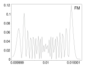
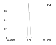
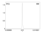
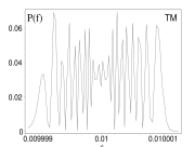
Figure 1: Power spectra showing the effects of frequency (FM), phase (PM) and amplitude (AM) modulation separately and all together (TM). The gravitational wave has frequency $10$ mHz.

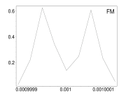
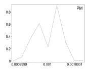
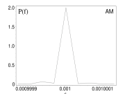
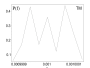
Figure 2: Power spectra showing the effects of frequency (FM), phase (PM) and amplitude (AM) modulation separately and all together (TM). The gravitational wave has frequency $1$ mHz.

One of the main effects of the modulations is to spread the power across a bandwidth $B\simeq 2(1+2\pi f\frac{R}{c}\sin\theta)f_{m}$. This, combined with LISA’s antenna pattern, means that the strain in the detector is often considerably less than the strain of the wave. The effect can be quantified in terms of the amplitude of the detector response, $A$, and the intrinsic amplitude of the source $\cal{A}$. Suppose that a source is responsible for a strain in the detector $s(t)$. Defining $A$ as the orbit-averaged response:

$$A^{2}=\frac{1}{T}\int_{0}^{T}s^{2}(t)\,dt,$$ (41)

we find from (7) that

$$A^{2}=\frac{1}{2}{\cal A}^{2}\left((1+\cos^{2}\imath)^{2}\langle F_{+}^{2}\rangle+4\cos^{2}\imath\langle F_{\times}^{2}\rangle\right),$$ (42)

where the orbit-averaged detector responses are given by

$$\langle F_{+}^{2}\rangle=\frac{1}{4}\left(\cos^{2}2\psi\langle D_{+}^{2}\rangle-\sin 4\psi\langle D_{+}D_{\times}\rangle+\sin^{2}2\psi\langle D_{\times}^{2}\rangle\right)$$

$$\langle F_{\times}^{2}\rangle=\frac{1}{4}\left(\cos^{2}2\psi\langle D_{\times}^{2}\rangle+\sin 4\psi\langle D_{+}D_{\times}\rangle+\sin^{2}2\psi\langle D_{+}^{2}\rangle\right)$$

$$\langle F_{+}F_{\times}\rangle=\frac{1}{8}\left(\sin 4\psi(\langle D_{+}^{2}\rangle-\langle D_{\times}^{2}\rangle)+2\cos 4\psi\langle D_{+}D_{\times}\rangle\right)$$

and

$$\langle D_{+}D_{\times}\rangle = \frac{243}{512}\cos\theta\sin 2\phi(2\cos^{2}\phi-1)(1+\cos^{2}\theta)$$

$$\langle D_{\times}^{2}\rangle = \frac{3}{512}\left(120\sin^{2}\theta+\cos^{2}\theta+162\sin^{2}2\phi\cos^{2}\theta\right)$$

$$\langle D_{+}^{2}\rangle = \frac{3}{2048}\left(487+158\cos^{2}\theta+7\cos^{4}\theta\right.$$ (44)

$$\left.\quad-162\sin^{2}2\phi(1+\cos^{2}\theta)^{2}\right)\,.$$

The relative amplitude $A/{\cal A}$ depends on the source declination $\theta$, right ascension $\phi$, inclination $\imath$ and polarization angle $\psi$.

Table 1: Properties of the six nearest interacting white dwarf binaries. Physical data from Hellier Hellier , periods taken from NSSDC catalog 5509NSSDC . Spectral amplitudes are computed using the methods of this paper for one year of observations. The masses quoted in units of the solar mass $M_{\odot}$, the orbital periods are in seconds, the distances are in parsecs and the strain spectral densities are in units of $10^{-19}$ Hz^-1/2.

Name	$\;m_{1}\;$	$\;m_{2}\;$	$\;P_{orb}\;$	$\;d\;$	$h_{f}^{B}$	$h_{f}^{D}$	$h_{f}^{D}/h_{f}^{B}$
AM CVn	$0.5$	$0.033$	$1028.76$	$100$	$21.2$	$2.34$	0.111
CP Eri	$0.6$	$0.02$	$1723.68$	$200$	$5.19$	$1.06$	0.205
CR Boo	$0.6$	$0.02$	$1471.31$	$100$	$11.5$	$1.63$	0.141
GP Com	$0.5$	$0.02$	$2791.58$	$200$	$3.32$	$0.44$	0.133
HP Lib	$0.6$	$0.03$	$1118.88$	$100$	$20.7$	$4.53$	0.219
V803 Cen	$0.6$	$0.02$	$1611.36$	$100$	$10.9$	$1.89$	0.174

Table 1 illustrates the power spreading effect for the six nearest interacting white dwarf binaries. Random numbers were used for the unknown parameters $\imath$ and $\psi$. The average strain spectral density in the detector, $h_{f}^{D}$, is between 5 and ten times below the strain spectral density at the barycenter $h_{f}^{B}$. The effect is more significant at higher frequencies since the bandwidth increases with frequency.

The signals from three of these binaries, averaged over their bandwidths, are plotted against the standard LISA noise curve in Figure 3. The complete signals for all six binaries are shown in Figure 4. The strain spectra appear as nearly vertical lines of dots due to the highly compressed frequency scale.

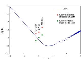
Figure 3: The strain spectral densities of three nearby interacting white dwarf binaries plotted against the standard LISA noise curve.

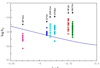
Figure 4: The modulated strain spectral densities of the six nearest interacting white dwarf binaries plotted against the standard LISA noise curve. Crosses mark standard estimates for the known binaries, while alternate symbols mark modulated Fourier components.

V Template Overlap

V.1 Template metric

The templates are constructed by choosing the six parameters $\vec{\lambda}\rightarrow(f,\theta,\phi,\imath,\psi,\varphi_{0})$ and forming the noise-free detector response corresponding to a source with those parameters:

$$s(t,\vec{\lambda})=A(t,\vec{\lambda})\cos\Psi(t,\vec{\lambda})$$ (45)

We need to determine how closely the templates need to be spaced to give a desired level of overlap. The overlap of templates with parameters $\vec{\lambda}_{1}$ and $\vec{\lambda}_{2}$ is defined:

$$R(\vec{\lambda}_{1},\vec{\lambda}_{2})=\frac{\langle s(t,\vec{\lambda}_{1})|s(t,\vec{\lambda}_{2})\rangle}{\langle s(t,\vec{\lambda}_{1})|s(t,\vec{\lambda}_{1})\rangle^{1/2}\langle s(t,\vec{\lambda}_{2})|s(t,\vec{\lambda}_{2})\rangle^{1/2}}\,,$$ (46)

with the inner product

$$\langle a(t)|b(t)\rangle=\int_{0}^{T}a(t)b(t)\,dt.$$ (47)

Suppose we have two templates, one with parameters $\vec{\lambda}$ and the other with parameters $\vec{\lambda}+\delta\vec{\lambda}$. To leading order in $\delta\vec{\lambda}$ the overlap is given by ben

$$R(\vec{\lambda},\vec{\lambda}+\delta\vec{\lambda})=1-g_{ij}(\vec{\lambda})\Delta\lambda^{i}\Delta\lambda^{j}$$ (48)

where $g_{ij}$ is the template space metric

$$g_{ij}(\vec{\lambda}) = \frac{\langle\partial_{i}s(t,\vec{\lambda})|\partial_{j}s(t,\vec{\lambda})\rangle}{2\langle s(t,\vec{\lambda})|s(t,\vec{\lambda})\rangle}$$ (49)

$$-\frac{\langle s(t,\vec{\lambda})|\partial_{i}s(t,\vec{\lambda})\rangle\langle s(t,\vec{\lambda})|\partial_{j}s(t,\vec{\lambda})\rangle}{2\langle s(t,\vec{\lambda})|s(t,\vec{\lambda})\rangle^{2}}\,.$$

Using the fact that $\Psi(t,\vec{\lambda})$ varies much faster than $A(t,\vec{\lambda})$ we find

$$g_{ij}(\vec{\lambda}) = \frac{\langle\partial_{i}A|\partial_{j}A\rangle+\langle A\partial_{i}\Psi|A\partial_{j}\Psi\rangle}{2\langle A|A\rangle}$$ (50)

$$-\frac{\langle A|\partial_{i}A\rangle\langle A|\partial_{j}A\rangle}{2\langle A|A\rangle^{2}}\,.$$

Ignoring the sub-dominant amplitude and phase modulation allows us to analytically compute the “Doppler metric”

$$ds^{2} = g_{ij}(\vec{\lambda})\Delta\lambda^{i}\Delta\lambda^{j}$$ (51)

$$= \frac{2\pi^{2}}{3}T^{2}df^{2}+\pi Tdfd\varphi_{0}+\frac{1}{2}d\varphi_{0}^{2}$$

$$-2\pi f\frac{R}{c}Tdf\left(\cos\theta\sin\phi d\theta+\sin\theta\cos\phi d\phi\right)$$

$$+\pi^{2}f^{2}\left(\frac{R}{c}\right)^{2}\left(\cos^{2}\theta d\theta^{2}+\sin^{2}\theta d\phi^{2}\right).$$

Here $T=1$ year is the observation time. We have to go beyond the Doppler approximation to find metric components that involve $\imath$ and $\psi$. The computations are considerably more involved, as are the resulting expression. For example, including all modulations we find

$$g_{\imath\imath}=\frac{2\langle F_{+}^{2}\rangle\langle F_{\times}^{2}\rangle\sin^{2}\imath\left(\sin^{2}\imath+2\cos^{4}\imath\right)}{\left((1+\cos^{2}\imath)^{2}\langle F_{+}^{2}\rangle+4\cos^{2}\imath\langle F_{\times}^{2}\rangle\right)^{2}}$$ (52)

and

$$g_{\psi\psi} = \frac{2(1+\cos^{2}\imath)^{2}\langle F_{\times}^{2}\rangle+4\cos^{2}\imath\langle F_{+}^{2}\rangle}{(1+\cos^{2}\imath)^{2}\langle F_{+}^{2}\rangle+4\cos^{2}\imath\langle F_{\times}^{2}\rangle}$$ (53)

$$-\frac{2\sin^{4}\imath\,\langle F_{+}F_{\times}\rangle}{\left((1+\cos^{2}\imath)^{2}\langle F_{+}^{2}\rangle+4\cos^{2}\imath\langle F_{\times}^{2}\rangle\right)^{2}}$$

We have been able to derived exact expressions for all the metric components, but they are cumbersome and not very informative. For most purposes the simple Doppler metric is sufficient.

V.2 Overlap of parameters

An important application of the Doppler metric in Eq. (51) is the determination of parameter overlap, which has great bearing on the placement of templates. In regions where large variations of the overlap can be seen for small changes in parameters, templates must be spaced closely to distinguish between different realizable physical situations. In regions where the change in overlap is small for small changes in parameters, the templates can be spaced more widely. The Doppler metric depends on only four parameters. Taking constant slices through the parameter space for any two of the four will produce a metric which can be used to plot level curves of the overlap function $R(\vec{\lambda}_{1},\vec{\lambda}_{2})$ as a function of two parameters.

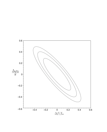
Figure 5: The template overlap contours on the $(f,\varphi_{0})$ cylinder.

Setting $d\theta=d\phi=0$ leaves the two dimensional metric on the $(f,\varphi_{0})$ cylinder:

$$ds^{2}_{2}=\frac{2}{3}\left(\frac{\pi}{f_{m}}df+\frac{3}{4}d\varphi_{0}\right)^{2}+\frac{1}{8}d\varphi_{0}^{2}\,.$$ (54)

Using this metric to plot the level sets of the overlap function, the contours for 90%, 80% and 70% overlap are shown in Figure 5. One rather surprising result is that the template overlap drops very quickly with $\Delta f$. According to Nyquist’s theorem, the frequency resolution observations of time $T$ should equal $f_{N}=1/T$. But we see from Figure 5 that the overlap drops to 90% for $\Delta f\sim f_{N}/10$. (Since we are using $T=1$ year, it so happens that the Nyquist frequency $f_{N}$ equals the modulation frequency $f_{m}$.)

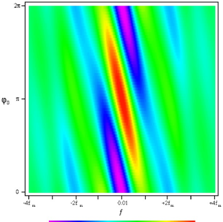
Figure 6: The overlap of templates with all parameters equal save frequency and orbital phase. The reference template has $(f,\varphi_{0})=(0.01,\pi)$. The frequency resolution was found to be independent of the reference frequency.

Since the metric (51) was derived by neglecting amplitude and phase modulation, it only gives an approximate determination of the template overlap. Moreover, the approximate metric neglects the $(\imath,\psi)$ dependence completely. In order to have a more reliable determination of the template overlap we generated a large template bank and studied the template overlap directly. We see that the template overlap shown in Figure 6 for $f$ vs. $\varphi_{0}$ agrees with what was found in Figure 5.

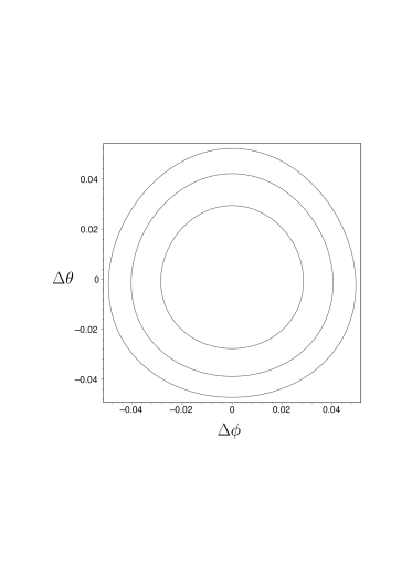
Figure 7: The template overlap contours on the sky 2-sphere in the neighborhood of $\theta=\pi/4$.

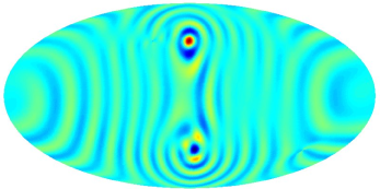
Figure 8: The overlap of templates with all parameters equal save sky position. The reference template has a frequency of $f=10$ mHz and a sky location of $(\theta,\phi)=(\pi/4,0)$.

Setting $df=d\varphi_{0}=0$ gives us the metric on the sky 2-sphere:

$$ds^{2}_{2}=\pi^{2}f^{2}\left(\frac{R}{c}\right)^{2}\left(\cos^{2}\theta d\theta^{2}+\sin^{2}\theta d\phi^{2}\right).$$ (55)

It is clear from this form of the metric that the angular resolution improves at higher frequencies, and that the metric is not that of a round 2-sphere. The $\cos^{2}\theta$ factor in front of $d\theta$ tells us that the $\theta$ resolution drops as we near the equator. This is might seem counter-intuitive since the Doppler modulation is maximal at the equator (it depends on $\sin\theta$). But, the $\theta$ resolution depends on the rate of change of the Doppler modulation with $\theta$, which goes as $\cos\theta$. Setting $f=10$ mHz, we plot the template overlap contours in the neighborhood of $\theta=\pi/4$ and $\theta=\pi/2$ in Figures 7 and 9 respectively.

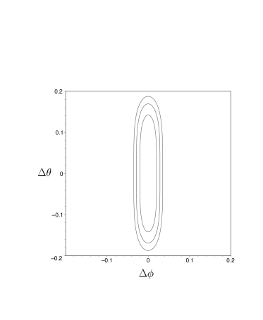
Figure 9: The template overlap contours on the sky 2-sphere in the neighborhood of $\theta=\pi/2$.

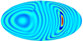
Figure 10: The overlap of templates with all parameters equal save sky position. The reference template has a frequency of $f=10$ mHz and is close to the galactic center, $(\theta,\phi)=(1.66742,4.65723)$.

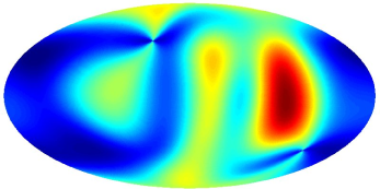
Figure 11: The overlap of templates with all parameters equal save sky position. The reference template has a frequency of $f=1$ mHz and is close to the galactic center, $(\theta,\phi)=(1.66742,4.65723)$.

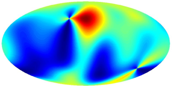
Figure 12: The overlap of templates with all parameters equal save sky position. The reference template has a frequency of $f=1$ mHz and a sky location of $(\theta,\phi)=(\pi/4,0)$.

The template overlaps shown in Figures 8 and 10 ($\theta$ vs. $\phi$) agree with those in found in Figures 7 and 9. The overlaps shown in Figures 11 and 12 (also $\theta$ vs. $\phi$) confirm our expectation that the angular resolution decreases with decreasing frequency.

The template overlap as a function of inclination and polarization angle turns out to be a very sensitive function of location in parameter space. While independent of frequency and orbital phase, the metric functions $g_{\imath\imath}$ and $g_{\psi\psi}$ range between 0 and 326 as $(\theta,\phi,\imath,\psi)$ are varied. Taking a uniform sample of $1.6\times 10^{9}$ points in $(\theta,\phi,\imath,\psi)$, we found that $g_{\imath\imath}$ had a mean value of $0.4664$, a median value of $0.043$, and that 90% of all points had $g_{\imath\imath}<1.273$. Similarly, $g_{\psi\psi}$ had a mean value of $2.101$, a median value of $2.0$, and that 90% of all points had $g_{\psi\psi}<2.251$. The analytic expressions for $g_{\psi\psi}$, $g_{\imath\imath}$ and $g_{\psi\imath}$ were found to agree with direct numerical calculations of the template overlap.

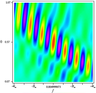
Figure 13: An example of non-local parameter degeneracies in the $f$, $\theta$ plane.

V.3 Degeneracies

What the metric can not tell us about are the non-local degeneracies that occur in parameter space. A mild example of a non-local degeneracy can be seen in Figure 8, where there are secondary maxima in the template overlap in the southern hemisphere. Physically this occurs because the dominant Doppler modulation is unable to distinguish between sources above and below the equator. This strong degeneracy is ameliorated by the amplitude and phase modulations, which are sensitive to which hemisphere the source is located in. In the course of applying the gCLEAN procedure we discovered several other much stronger non-local parameter degeneracies. By far the worst were those that involved frequency and sky location. The secondary maxima sometimes had overlaps as high as 90%. An example of a non-local parameter degeneracy in the $f$ - $\theta$ plane is shown in Figure 13. The reference template has $f=4.999873$ mHz, $\theta=0.5690$, $\phi=0.643$, $\imath=1.57$, $\psi=0.314$, and $\varphi_{0}=0.50$. The strongest of the secondary maxima is located at $f=4.999910$ mHz, $\theta=0.4615$, and has an overlap of 90% with the reference template. In principle, a sufficiently fine template grid should always find the global maxima, but in practice, detector noise and interference from other sources can cause gCLEAN to use templates from secondary maxima. We will return to this issue when discussing the source identification and reconstruction procedure.

V.4 Counting templates

Deciding what level of template spacing is acceptable depends on two factors: the signal-to-noise level and computing resources. Given a signal-to-noise level of SNR, there is no point having the template overlap exceeding $\sim(1-1/{\rm SNR})\times 100$%. For the searches described in the next section we made a trade-off between coverage and speed, and chose template spacings that gave a minimum template overlap of $\sim 75\%$ in each parameter direction (i.e. with all parameters equal save the one that is varied). We chose to study sources with frequencies near 5 mHz, and used a uniform template grid with spacings $\Delta f=f_{m}/5$, $\Delta\varphi_{0}=\pi/4$, $\Delta\theta=\Delta\phi=3.7^{o}$, $\Delta\imath=\pi/7$ and $\Delta\psi=\pi/9$. A better approach would be to vary the template spacing according to where the templates lie in parameter space. As explained earlier, each set of $5\times 4\times 3072\times 7\times 9=3,870,720$ templates can be used to cover a frequency range of $10^{4}f_{m}$. At worst, a source may lie half way between two templates, so a $\sim 75\%$ template overlap translates into a $\sim 92\%$ source overlap. After the coarse template bank has been used to find a best match with the data, we refine the search in the neighborhood of the best match using templates that are spaced twice as finely in each parameter direction.

To implement the gCLEAN procedure, a template bank was constructed by gridding the sky using the HEALPIX hierarchical, equal area pixelization scheme HEALpix . The HEALPIX centers provide sky locations $(\theta,\phi)$ to build up families of templates distributed across the parameters $(f,\imath,\psi,\varphi_{0})$.

VI Instrument Noise

In order to construct a demonstration of the gCLEAN method, it is necessary not only to characterize the binary signals themselves, but also the noise in the detector. Instrumental noise can have important consequences for the gCLEAN process, particularly in low signal to noise ratio situations, where random features in the noise spectrum of the instrument could conspire to approximate the modulated signal from a binary.

The total output of the interferometer is given by the sum of the signal and the noise:

$$h(t)=s(t)+n(t)\,.$$ (56)

Assuming the noise is Gaussian, it can be fully characterized by the expectation values

$$\langle\tilde{n}(f)\rangle=0\,,\quad{\rm and}\quad\langle\tilde{n}^{*}(f)\tilde{n}(f^{\prime})\rangle=\frac{1}{2}\delta(f-f^{\prime})S_{n}(f)\,,$$ (57)

where $S_{n}(f)$ is the one-sided noise power spectral density. It is defined by

$$\langle n^{2}(t)\rangle=\int_{0}^{\infty}dfS_{n}(f)\ ,$$ (58)

where the angle brackets denote an ensemble average. The one-sided power spectral density is related to the strain spectral density by $S_{n}(f)=|\tilde{h}_{n}(f)|^{2}$.

Expressing the noise as a discrete Fourier transform:

$$n(t)=\sum_{j}n_{j}e^{2\pi if_{m}jt},$$ (59)

a realization of the noise can be made by drawing the real and imaginary parts of $n_{j}$ from a Gaussian distribution with zero mean and standard deviation

$$\sigma_{j}=\frac{\tilde{h}_{n}(f_{m}j)}{\sqrt{2}}\,.$$ (60)

The signal-to-noise ratio in a gravitational wave detector is traditionally defined as

$${\rm SNR}(f)=\sqrt{\frac{S_{s}(f)}{S_{n}(f)}}\,,$$ (61)

where $S_{s}(f)$ is the one-sided power spectral density of the instrumental signal. Given a particular set of sources, each with their own modulation pattern, and a particular realization of the noise, the quantity ${\rm SNR}(f)$ will vary wildly from bin to bin. A more useful quantity is obtained by comparing the signal to noise over some frequency interval of width $\Delta f$ centered at $f$:

$${\rm SNR}(f,\Delta f)=\sqrt{\frac{\{S_{s}(f)\}}{\{S_{n}(f)\}}}\,,$$ (62)

where

$$\{S(f)\}=\int_{f-\Delta f/2}^{f+\Delta f/2}S(x)\,dx\,.$$ (63)

A good choice is to set $\Delta f$ equal to the typical bandwidth of a source.

VII Source identification and subtraction

The procedure for subtraction is intimately tied to the task of source identification, as sources with overlapping bandwidths interfere with each other. Overlapping sources have to be identified and removed in a simultaneous, iterative procedure called the gCLEAN algorithm.

The task of gCLEAN can be understood by thinking of the LISA data stream as an $N$ dimensional vector $\vec{S}$ which represents the sum of all the sources the algorithm is seeking to subtract. $\vec{S}$ is called the total source vector. The ideal output of the gCLEAN algorithm is a set of basis vectors and their amplitudes (i.e., sources $\vec{s}_{i}$) which contribute to $\vec{S}$:

$$\vec{S}=\vec{s}_{1}+\vec{s}_{2}+\dots\ .$$ (64)

The basis vectors which contribute to individual sources $\vec{s}_{i}$ are the unit-normed templates on the parameter space, ${\hat{t}}_{j}$, built from Eq. (34). In principle, the vector space of templates will be quite large, where the number of basis vectors $M$ is much greater than the dimensionality $N$ of the source vector.

A typical application may attempt to CLEAN a frequency window of width $\Delta f$. The source vector $\vec{S}$ has dimension $N=2\Delta f/f_{N}$, where the factor of two accounts for the real and imaginary parts of the Fourier signal. We typically considered frequency windows of size $\Delta f\approx 1\;\mu{\rm Hz}$ and observation times of $T=1$ year, so $N\approx 60$. By contrast, the number of templates used in a search over that data stream is of order $10^{8}$. This discrepancy in size naturally leads to the possibility of multiple solutions, implying that the problem is ill posed. What gCLEAN does is return a best-fit solution in much the same vein as a singular value decomposition.

VII.1 CLEANing

The first step in the gCLEAN procedure is to consider the inner product of each template ${\hat{t}}_{i}$ with the source vector $\vec{S}$, which represents the data stream from the interferometer. The “best fit” template, ${\hat{t}}_{j}$, is identified as the template with the largest overlap with $\vec{S}$, and a small amount $\epsilon$ is subtracted off:

$$\vec{S}^{\prime}=\vec{S}-\epsilon(\vec{S}\cdot\hat{t}_{j})\hat{t}_{j}\,,$$ (65)

where $(\vec{S}\cdot\hat{t}_{j})\hat{t}_{j}$ is gCLEAN’s best estimate of $\vec{S}$. The template ${\hat{t}}_{j}$ and amount removed are recorded for later reconstruction.

The procedure is iterated until only a small fraction of the original power remains (for the simulations presented below, the fraction was chosen to be $1\%$). It should be emphasized that the data stream that remains after this process is not the CLEANed data stream. By design gCLEAN will remove a pre-set fraction of the original power, no matter what the original signal is composed of. It is only after reconstructing the sources from the gCLEAN record that we can meaningfully attempt to remove a source from the data stream.

The pieces which are subtracted off in the gCLEAN procedure are assumed to be portions of individual sources $\vec{s}_{i}$, the ensemble of which form the total signal $\vec{S}$; during reconstruction these pieces are resummed into representations of the individual sources.

VII.2 Reconstruction

The gCLEAN procedure cannot produce a perfect match with a raw data stream from LISA, due to the discrete griding of parameter space, the interference between the frequency components of different sources and instrument noise. These effects serve to generate subtracted elements which are close, but not identical to each other. The task during reconstruction is to identify which combination of subtracted elements are close enough together that they are considered to be manifestations of a single source.

Reconstruction is implemented by finding the brightest element in the list of saved matches produced by gCLEAN, and computing the overlap of this element with all other saved elements. For a given overlap threshold, all sources with strong overlap are considered to be “close”, and are summed together to represent a single source. The procedure is iterated over the remaining saved elements until every element in the gCLEAN record has contributed to a source. The frequency and source location parameters for the reconstructed sources are taken to be a weighted average of all the matches contributing to that source, where the weighting is given by the individual match amplitudes.

The procedure is complicated by the non-local parameter degeneracies discussed in section V.2. The reconstruction may combine contributions that are close in terms of template overlap, but far apart in terms of the template metric. It makes no sense to average the parameters of metrically distant templates. For this reason we only use contributions that are metrically close when calculating the weighted averages of the source parameters. This can lead to several different best fit values for the reconstructed source.

We encounter an additional difficulty when trying to reconstruct the source amplitudes $A$ and ${\cal A}$. Consider a source with amplitude $A$. If gCLEAN performs $n$ subtractions from this source the remaining amplitude will be

$$A_{n}\approx A(1-\epsilon)^{n}\,.$$ (66)

The equation is only approximate as other reconstructed sources may have added or subtracted from the source in question during the course of the gCLEAN procedure. If we simply add together the $n$ contributions identified by gCLEAN, the amplitude of the reconstructed source will equal

$$A_{r}\approx A\left(1-(1-\epsilon)^{n}\right)\,.$$ (67)

In other words, gCLEAN will tend to under estimate the amplitude of a source. To compensate, we multiply the initial reconstruction by a factor of $1/\left(1-(1-\epsilon)^{n}\right)$ to arrive at the final reconstruction which gives a better estimate of $A$. Using this estimate, along with the weighted averages for $(\theta,\phi,\imath,\psi)$, we can use Equation 42 to calculate ${\cal A}$. Unfortunately, any errors in the determination of $(A,\theta,\phi,\imath,\psi)$ adversely affect our determination of ${\cal A}$. Because of this, the intrinsic amplitude of a source, ${\cal A}$, is usually the worst determined quantity.

The reconstruction procedure usually produces more reconstructed sources than there were sources in the input data stream. Most of these additional “sources” have very small amplitudes, and their existence can be attributed to detector noise or the formation of a blended version of two or more real sources. For this reason, we only consider reconstructed sources with an amplitude that exceeds the noise in the detector. Occasionally gCLEAN gets confused and produces two fits to a single source that are nearby in parameter space, but not close enough to have been identified as one source. We discuss some ideas for getting around this problem in Section VIII.

VII.3 Isolated Sources

Figure 14 shows the result of a gCLEAN run carried out for an isolated source. The source parameters are listed in table 2. The strain spectral density of the source and detector noise are shown in Figure 14, along with the composite source built by gCLEAN. The signal to noise ratio was $9.75$ across the bandwidth of the signal.

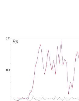
Figure 14: The solid line is the strain spectral density of the source, the dotted line is that of the noise and the dashed line indicates the strain spectral density of the composite source created by gCLEAN.

The output from gCLEAN was then fed through the reconstruction procedure using an overlap threshold of $0.7$. The source parameters were estimated by taking a weighted average of the template parameters used to create the composite source. These estimates are listed in table 2. The reconstruction procedure was able to fit all of the source parameters very well save for the intrinsic amplitude ${\cal A}$. The error in ${\cal A}$ is primarily due to the error in the inclination. The large error in ${\cal A}$ translates into a large error in the distance to the source $d$. The reconstructed parameter values for the source can be fed into our detector response model, and the resulting strain can be subtracted from the data stream. The CLEANed data stream is shown in Figure 15. The residual is comparable to the noise in the detector.

Table 2: The parameters for the isolated source example. The first row lists the input values while the second row list the reconstructed values.

$f$ (mHz)	${\cal A}$	$A$	$\theta$	$\phi$	$\imath$	$\psi$	$\varphi_{0}$
5.000281	0.556	0.648	0.79	2.21	2.45	1.62	0.71
5.000280	0.786	0.646	0.79	2.21	2.11	1.63	0.81

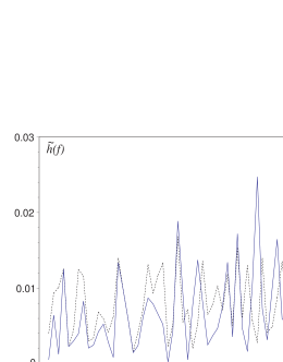
Figure 15: The solid line is the CLEANed strain spectral density and the dotted line is the original detector noise.

What we have shown is that the gCLEAN procedure is able to successfully remove isolated sources from the LISA data stream. The procedure works equally well if there are one or one million isolated sources. The key is that the sources are isolated, i.e. the signals do not overlap in Fourier space. When the sources are overlapping they interfere with each other and the CLEANing is more difficult.

VII.4 Overlapping Sources

Table 3: The source parameters used to generate the overlapping signals.

$\#$	$f$ (mHz)	SNR	${\cal A}$	$A$	$\theta$	$\phi$	$\imath$	$\psi$	$\varphi_{0}$
1	4.999729	14.3	0.514	0.741	0.66	3.32	2.86	1.42	1.84
2	4.999904	7.7	0.322	0.399	2.87	0.26	2.64	0.26	2.00
3	5.000216	8.8	0.829	0.457	1.40	4.35	1.57	1.10	1.18

To get a feel for how the gCLEAN procedure copes with overlapping sources, we considered three sources with barycenter frequencies near 5 mHz that are within $\sim 5$ frequency bins of each other. The total signal to noise in the simulation was equal to ${\rm SNR}=19.5$. Table 3 list the randomly generated source parameters and the signal-to-noise ratio for each source. The modulations described in Section II cause the measured strains to overlap in frequency space. The composite strain spectral density produced by the three sources is shown in Figure 16, along with the detector noise used in the simulation. Also shown is the residual strain after the three reconstructed sources have been subtracted from the original data stream.

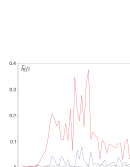
Figure 16: The strain spectral density for the overlapping source example. The solid line is the signal, the dashed line is the residual strain (i.e. the CLEANed signal), and the dotted line is the detector noise.

The usual procedure was followed: The simulated LISA data stream was fed into the gCLEAN algorithm, and the output from the gCLEAN run was used to reconstruct the sources. An overlap threshold of $0.7$ was used in the reconstruction. The reconstruction produced five reconstructed sources with signal to noise ratios greater than one. The reconstructed source parameters are listed in Table 4. The first three reconstructed sources are fair reproductions of the input sources. The frequencies and sky locations are well determined, but there are larger errors in the determination of the inclination, polarization angle, and orbital phase. The strain amplitude in the detector, $A$, is fairly well determined for sources 1 and 2, but poorly determined for source 3. Once again, the intrinsic amplitude of each source, ${\cal A}$, is the least well determined parameter.

Table 4: The reconstructed sources

$\#$	$f$ (mHz)	$A_{r}$	${\cal A}$	$A$	$\theta$	$\phi$	$\imath$	$\psi$	$\varphi_{0}$
1	4.999729	0.646	0.942	0.731	0.67	3.33	1.98	1.10	1.22
2	4.999910	0.204	0.477	0.343	2.85	0.42	1.79	0.44	1.10
3	5.000214	0.163	0.543	0.314	1.50	4.37	1.57	1.04	1.49
4	5.000089	0.061	0.868	0.320	2.63	5.33	1.42	2.88	1.67
5	5.000336	0.050	0.217	0.177	2.36	4.12	1.98	0.98	1.78

In addition to recovering the three input sources, the reconstruction procedure produced two spurious sources. The degree to which these sources were used by the gCLEAN procedure is measured by the amplitude $A_{r}$. It is clear from the $A_{r}$ values that the first three reconstructed sources played a much more significant role in the gCLEAN procedure than the two spurious sources. In terms of the amount of signal removed during the the gCLEAN procedure, the reconstructed sources had signal to noise ratios of $12.1$, $3.9$, $4.3$, $1.6$, and $1.1$ respectively. This suggests that we should only consider sources with signal to noise ratios above ${\rm SNR}\sim 2$ when performing the reconstruction. Our hope is that, when we implement some of the improvements described in Section VIII, the CLEANing procedure will produce fewer and weaker spurious reconstructions.

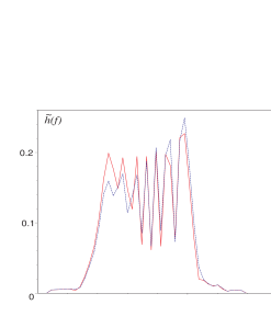
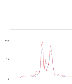
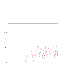
Figure 17: The strain spectral densities of the three sources (solid lines) and their reconstructions (dashed lines).

The strain spectral densities for the sources and their reconstructions are shown in Figure 17. The reconstruction procedure underestimates the amplitudes of sources 2 and 3. This can be attributed to the power lost to spurious sources in the gCLEAN procedure. The CLEANed strain spectral density shown in Figure 16 was produced by subtracting the three reconstructed sources shown in Figure 17 from the input data stream. The residual strain is down by a factor of $\sim 10$ from the input level, but is still considerably larger than the detector noise. The goal of future work will be to improve the source identification and subtraction procedure to the point where multiple sources with overlapping signals can be removed from the LISA data stream leaving a residual that is comparable to the instrument noise.

VIII Future Work

The gCLEAN algorithm described here is only the first step in a program to understand how to remove binaries from the LISA data stream. In particular, the limitation of the simulations presented here are for small numbers of binaries, and at frequencies above the expected regime where multiple overlapping binaries contribute power in every bin of the power spectrum (this occurs at $f\simeq 3$ mHz, for an assumed bin width of $f_{N}\simeq 1/{\rm year}$).

A key question is how effectively can gCLEAN identify binaries which have merged together to form a confusion limited background? While gCLEAN will subtract any signal out of the data stream down to a prescribed level in total power, using as many templates as necessary to remove the “signal”, the real question is how well can it identify individual sources for later removal? Information theory predicts an ultimate bound on the number of binaries which can be fit out of the LISA data stream sterl , and an important question is how closely can gCLEAN approach this optimal limit.

A great deal of work has yet to be done in the area of optimizing the gCLEAN procedure and making it an effective tool in the LISA data analysis arsenal; many of them are obvious extensions to the initial foray presented in this work. Of particular interest is extending gCLEAN to work with multiple data streams. The design of the LISA observatory provides three different data streams, which can be combined in various ways . As currently implemented, gCLEAN only uses a single data stream. We are in the process of upgrading the algorithm so that all data streams are used. It is our hope that some of the parameter degeneracies described in Section V.3 will be broken when more than one interferometer signal is used. At the very least, we expect the parameter estimation to be improved. It would also be interesting to see how much better the algorithm performs if we use more than one year of observations.

The placement of templates in parameter space is an area where improvements in efficiency can be implemented. Templates now are spaced for convenience (e.g., points on the sky are spaced on the HEALPIX centers, which are effective for visualization), but efficient template spacing should be developed based on the local values of the metric on the template space.

There are also several unresolved questions about the gCLEAN algorithm and the ultimate limits of its performance on real scientific data. Of particular interest is how will gCLEAN perform when other signals, such as those from supermassive black hole binaries, are present in the data? The research presented here has been for the case where only circular Newtonian binaries are present in the data stream. It is clear from the way gCLEAN is designed to work that it will indiscriminately remove signals from a data stream; this has important implications for how gCLEAN should be included in the approach to LISA data analysis. How will gCLEAN deal with chirping binaries, or signals from extreme-mass ratio inspirals? Can gCLEAN be used in a sequential analysis strategy, where it is used to first subtract out monochromatic binaries before looking for other gravitational wave events, or do all signals have to be simultaneously gCLEANed using templates for each individual type of source?

There may be better ways to extract the best fit parameter values for the reconstructed sources. Currently we use a weighted average of the parameters that describe the templates used to build up the reconstructed source. A better approach may be to take each reconstructed source and use a hierarchical search through parameter space to find which set of parameters give the best match to the reconstructed source.

Another avenue of research is devising better strategies for accurately fitting sources. One idea is to attempt multi-fitting, where gCLEAN removes more than one source at a time. The parameter space scales as $6^{n}$, where $n$ is the number of sources which the algorithm is attempting to subtract out at once. With this in mind, it is obvious that one would have to establish initial estimates of the parameters from a standard gCLEAN pass in order to narrow the search area of the parameter space used in the multi-fitting. An aspect of the subtraction enterprise which might benefit from such a procedure is what to do with orphaned sources which are generated during reconstruction but do not meet the threshold requirements to be included in the final list of identified sources. These orphans represent subtractions on the part of gCLEAN which arise from either fluctuations in the detector noise which produces a close match with templates, or more commonly, interference between the signals of multiple sources which produced a strong match during the gCLEAN iterations. This type of subtraction is inevitable, as gCLEAN has no a priori way of distinguishing interfering sources from isolated sources; it relies only on its ability to match the current version of the data stream to its space of templates.

There are many obvious avenues of refinement which should be pursued in future work to develop the gCLEAN algorithm. We are working on several of the issues described above, and we encourage others to pursue aspects of the problem which are of interest to them. To aid in the exploration of the strengths and weaknesses of the gCLEAN algorithm, the analysis codes used to produce the results in this paper will be made available to the scientific community through the Working Groups of the LISA project.

References

- (1) P. L. Bender & D. Hils, Class. Quantum Grav. 14, 1439 (1997).
- (2) D. Hils, P. Bender, & R. F. Webbink, Astrophys. J. 360, 75 (1990).
- (3) P. Bender et al., LISA Pre-Phase A Report (Second Edition)(1998)(unpublished).
- (4) C. J. Hogan & P. L. Bender, Phys. Rev. D 64, 062002 (2001).
- (5) N. J. Cornish & S. Larson, preprint gr-qc/0206017, accepted in Class. Quant. Grav. (2002).
- (6) S. A. Hughes, Phys. Rev. D 64, 064004 (2001).
- (7) K. Glampedakis, S. A. Hughes & D. Kennefick, preprint gr-qc/0205033, submitted to Phys. Rev. D (2002).
- (8) C. Cutler, Phys. Rev. D 57, 7089 (1998).
- (9) T. Moore & R. W. Hellings, Phys. Rev. D 65, 06201 (2002).
- (10) R. T. Stebbins, D. Hils, B. K. Bender & P. L. Bender, Talk given at the Third International LISA Symposium, July (2000).
- (11) J. Högbom, Astr. J. Suppl. 15, 417 (1974).
- (12) N. J. Cornish & L. J. Rubbo, Phys. Rev. D 67, 022001 (2003).
- (13) N. J. Cornish & S. Larson, Class. Quantum Grav. 18, 3473 (2001).
- (14) P. C. Peters & J. Mathews, Phys. Rev. 131, 435 (1963).
- (15) C. Hellier, Cataclysmic variable stars, Springer-Praxis, London (2001).
- (16) National Space Science Data Center http://nssdc.gsfc.nasa.gov/.
- (17) B. Owen, Phys. Rev. D 53, 6749 (1996).
- (18) K. M. Gorski, B. D. Wandelt, E. Hivon, F. K. Hansen & A. J. Banday, astro-ph/9905275 (1999) and http://www.eso.org/science/healpix/.
- (19) S. Phinney, Talk given at the Fourth International LISA Symposium, July (2002).