A weakly non-adiabatic one-zone model of stellar pulsations: application to Mira stars

Abstract

There is growing observational evidence that the irregular changes in the light curves of certain variable stars might be due to deterministic chaos. Supporting these conclusions, several simple models of non-linear oscillators have been shown to be capable of reproducing the observed complex behaviour. In this work, we introduce a non-linear, non-adiabatic one-zone model intended to reveal the factors leading to irregular luminosity variations in some pulsating stars. We have studied and characterized the dynamical behaviour of the oscillator as the input parameters are varied. The parametric study implied values corresponding to stellar models in the family of Long Period Variables and in particular of Mira-type stars. We draw the attention on certain solutions that reproduce with reasonable accuracy the observed behaviour of some peculiar Mira variables.

1 Introduction

The region in the Hertzsprung–Russell diagram which provides the majority and, probably, the most interesting classes of pulsating stars is the Asymptotic Giant Branch (AGB). As the stars of low and intermediate mass (from say $\sim 1$ to $11\,M_{\odot}$) evolve along the AGB phase, they experience recurrent thermal instabilities and substantial mass loss. Depending on the phase in the thermal pulse cycle, they may spend intermittent time intervals as pulsating stars (Groenewegen & Jong 1994). As a consequence, they eject freshly synthesized material into the interstellar medium. Thus, they also play a crucial role for our understanding of the chemical evolution of galaxies. Last but not least, the corresponding stellar models are basic tools to study how planetary nebulae and their central objects form — see Habbing (1996) and Willson (2000) for reviews on the subject.

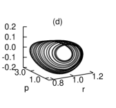
Figure 1: Period-doubling route to chaos represented in the space $(r,v,p)$. In all panels, $\alpha=0.1$, $\omega=20.1$, and $a=20$ have been adopted. (a) $\xi=0.08$: Period-1; (b) $\xi=0.09$: Period-2; (c) $\xi=0.108$: Period:4; (d) $\xi=0.12$: Chaos.

A substantial number of pulsating stars in the Galaxy show irregular behaviour and have the characteristics of AGB stars (Wood 2003). This makes them an interesting research target for theoretical modeling. The work done so far on non-linear stellar pulsations can be grouped into two different categories: the full numerical hydrodynamical approach and the more straightforward approach of the theory of dynamical systems. The former is directly based on an extensive knowledge of the physical processes in the star — equation of state, opacities, and many more — and requires the implementation of a hydrodynamical code coupled with a detailed treatment of the transfer of radiation. Hence, this approach definitely provides the most detailed and accurate description of pulsations. However, within this framework it is sometimes difficult to interpret the origin and shapes of the resulting light curves as the stellar parameters are varied. On its hand, the second approach is complementary to the former in the sense that it gives a qualitative framework in which the general features of the pulsations are easily understood and, consequently, allows to develop intuitive explanations in terms of a few very basic and relatively simple physical processes (Buchler 1993).

The hydrodynamic simulations of pulsating stars succeeded in reproducing the phenomenon of period-doubling (Buchler & Kóvacs 1987; Kóvacs & Buchler 1988; Aikawa 1990) and tangent bifurcations (Buchler, Goupil & Kóvacs 1987; Aikawa 1987) found in the light curves of some specific stars by changing the surface temperature or surface gravity. In particular, it has been found that there is strong evidence of underlying low-dimensional chaos from the non-linear analysis of the light curves of the irregular stars R Sct, AC Her, and SX Her (Buchler, Kolláth & Cadmus 2001). This paved the road to construct simple models within the framework of the theory of dynamical systems which turned out to be capable of reproducing the complex behaviour. Within this approach perhaps the simplest models of stellar pulsations are the so-called one-zone models. In this family of models the star is treated as a rigid core surrounded by a homogeneous gas shell. The one-zone models are not intended to be a substitute for fully hydrodynamical and sophisticated models. Instead, they merely seek a global and qualitative explanation of what process might be at the root of the chaotic behaviour. In the present paper, we propose a one-zone model of non-linear non-adiabatic stellar oscillations. We present the parametric study of the system and draw the attention on a particular set of numerical solutions which may have implications in the study of the variability of Long Period Variables (LPVs).

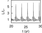
Figure 2: The birth of a knot-like structure for increasing values of $Q$. Top panels: Stroboscopic sampling of the orbit ($r,v,p$) with the characteristic frequency $\omega$: (a) $Q=1.02$, (b) $Q=1.04$, (c) $Q=1.08$ and (d) $Q=1.16$. Bottom panels: The light curves corresponding to the cases shown in the upper panels.

2 The one-zone model

Baker et al. (1966) were the first to introduce the one-zone model as tool to study the nonlinear behaviour of stellar pulsations. Buchler & Regev (1982) and Auvergne & Baglin (1985) later studied one-zone models under the assumption that the nonlinearity of the adiabatic coefficient $\Gamma_{1}$ is the main trigger for nonlinear pulsations, whereas Tanaka & Takeuti (1988) pointed out that dynamical stability might be necessary for realistic models of pulsating stars, which is the approach followed here.

The one-zone model approach is especially suited for the AGB stars as the density difference between the central core and the outer layers is so large that these two regions can be considered as effectively decoupled. Following Icke et al. (1992) and Munteanu et al. (2002), we consider the stellar pulsation to be simulated by a variable inner boundary located well beneath the photosphere and moving with constant frequency (piston approximation). This sinusoidal driving consists of pressure waves originating in the interior and propagating through a transition zone until they dissipate in the outer layers. We denominate the driving oscillator “the interior” and the driven oscillator “the mantle”. While the radius of the former region, $R_{0}$, can be estimated as the radius of the hydrogen burning shell, the radius of the latter, $R$ is determined by the dissipation of the aforementioned pressure waves.

The variation of the interior radius, $R_{\rm c}$, around the equilibrium value, $R_{0}$, is given by $R_{\rm c}=R_{0}+\alpha R_{0}~{}\sin~{}\omega_{\rm c}\tau$, where $\alpha$ and $\omega_{\rm c}$ are, respectively, the fractional amplitude and the frequency of the driving. As in Stellingwerf (1972), we use the equation of motion and the energy equation without energy sources and in absence of any driving force in order to determine the final equation of motion describing the dynamics of the mantle. In the present work, we will study the particular case in which the luminosity at the base of the mantle equals the (constant) equilibrium luminosity of the star, $L_{\star}$. For convenience, we use as variables the non-dimensional radius $r\equiv R/R_{\star}$, pressure $p\equiv P/P_{\star}$ and time $t\equiv\omega_{\rm m}\tau$, where the stellar radius and pressure were normalized to their equilibrium values, while

$$\omega_{\rm m}\equiv\sqrt{\frac{GM}{R_{\star}^{3}}}$$ (1)

is the characteristic frequency of the star.

Considering that the additional perturbative acceleration is proportional to the driving acceleration with a transmission coefficient $Q$ as in Icke et al. (1992) and following the reasoning of Saitou, Takeuti & Tanaka (1989) for the energy equation, we obtain the following equation of motion

$$\frac{dr}{dt} = v$$

$$\frac{dv}{dt} = p\,r^{2}-r^{-2}-$$

$$~{}~{}~{}~{}~{}-Q\alpha\omega^{4/3}\sin(\omega r-\omega t-\alpha\omega^{1/3}\sin\omega t)$$ (2)

$$\frac{dp}{dt} = -3\Gamma_{1}r^{-1}vp-\xi r^{-3}(r^{\beta}p^{\delta}-1),$$

where

$$\beta=a(r^{3}p-1.2)+21.6~{}~{},~{}~{}\delta=3.6r^{3}p(r^{3}p-0.2)$$ (3)

are the coefficients introduced in Saitou et al. (1989) as a saturation effect of the $\kappa$-mechanism with $a$ being the control parameter. The characteristic frequency of the perturbation, $\omega$ results from the use of the dimensionless time unit and from the assumption that $R_{0}$ encompasses almost the entire stellar mass. It is defined as

$$\omega\equiv\frac{\omega_{\rm c}}{\omega_{\rm m}}=\left(\frac{R_{0}}{R_{\star}}\right)^{-3/2}.$$ (4)

In its simplest form, the study of stellar pulsations can be considered as a thermo-mechanical, coupled oscillator problem (Gautschy & Glatzel 1990). The coupling constant is given by the ratio of the dynamical to the thermal time scale in the outer layers of the star. Whenever the thermal time scale ($\tau_{\rm th}\sim 4\pi r^{2}\rho\Delta rc_{\rm V}T/L_{\rm r}$) of an outer region of the star of radial extension $\Delta r$ happens to become comparable to the sound-traveling time through that region ($\tau_{\rm dyn}\sim\Delta r/c_{\rm s}$), non-adiabatic effects are relevant. This implies that there is an efficient exchange of mechanical and thermal energies in that region. The ratio of the time scales is much smaller than one throughout most of the envelope and is close to unity only in the outermost regions. Significant non-adiabatic effects are relevant for helium stars, very massive AGB stars, some post-AGB stars and in the ionization zones of hot stars (Stellingwerf 1986; Gautschy & Saio 1995). In the context of our system, the parameter $\xi$ in Eq.(2) is a measure of the non-adiabaticity and is given by the ratio of the dynamical timescale to the thermal timescale of the shell

$$\xi~{}=~{}\frac{L_{\star}}{\omega_{m}c_{\rm V}mT}.$$ (5)

The system of Eq.(2) constitutes the final set of relations for the unknowns $r$, $v$ and $p$. The parameters that must be specified are $Q$, $\alpha$, $\omega$, $\Gamma_{1}$, $a$ and $\xi$. We consider an ideal gas with an adiabatic coefficient $\Gamma_{1}=5/3$. The parameter fixing the evolutionary status of the star is $\omega$ as it provides a measure of the contrast between the core and the envelope. For AGB stars, $R_{0}/R_{\star}$ is of the order of 15%. This led Icke et al. (1992) to consider a value of $\omega=20.1$ which is the value adopted here. We have performed a parametric study involving the parameters of the perturbation, $Q$ and $\alpha$. The results of the numerical integrations show that the pair $(Q,\alpha)$ — and not the individual specific values of $Q$ and $\alpha$ — determines the dynamics of the system. In other words, given a fixed value of $\alpha$, a certain range of values of $Q$ can be found for which the same peculiar dynamics discussed below develops. Therefore, we present here only the case of small internal perturbation ($\alpha\approx 3-4\%$) and amplified transmission through the envelope $(Q>1)$. It is worth noticing that for higher (lower) values of the parameter $\alpha$, the same behaviour is encountered if lower (higher) values of the coupling coefficient $Q$ are chosen.

3 Numerical results

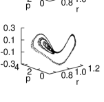
Figure 3: Comparison between regular and irregular dynamics. The light curves and the corresponding stroboscopic maps for the cases $\alpha=0.037$, $\omega=20.1$ and (top panels) $Q=0.8$, (middle panels) $Q=1.0$ and (bottom panels) $Q=1.048$.

3.1 Zero perturbation

The system studied by Saitou et al. (1989) can be obtained from the system given in (2) by considering the case of zero perturbation ($Q=0$). In spite of the inexistence of internal perturbation, this system is the prototype of non-linear self-excited oscillators due the $\kappa$-mechanism provided that $\xi\neq 0$. The behaviour of any dynamical system $\mbox{\boldmath$\dot{x}$}=\mbox{\boldmath$F$}(\mbox{\boldmath$x$})$, with $\mbox{\boldmath$x$}=(x_{1},x_{2},...,x_{n})$ and $\mbox{\boldmath$F$}=(F_{1},F_{2},...,F_{n})$ is critically determined by its fixed points $\mbox{\boldmath$x$}_{0}$ given by $\mbox{\boldmath$F$}(\mbox{\boldmath$x$}_{0})=0$. The associated eigenvalues of the Jacobian matrix $(J_{\mbox{\boldmath$x$}_{0}})_{ij}=(\partial F_{i}/\partial x_{j})_{\mbox{\boldmath$x$}_{0}}$ determine the nature of these fixed points. For instance, for a fixed point to be stable, it is required that all eigenvalues have negative real parts. In our case, the system has three fixed points: a trivial one, $(r_{0},v_{0},p_{0})=(1,0,1)$, with mainly adiabatic origin and two other fixed points, $(r_{0}^{+},v_{0}^{+},p_{0}^{+})\approx(0.68,0,4.75)$ and $(r_{0}^{-},v_{0}^{-},p_{0}^{-})\approx(8.8558,0,0002)$, entirely due to non-adiabatic effects (that is, they exist only for $\xi\neq 0$). For initial conditions close to the trivial fixed point, the period-doubling route to chaos was obtained by Saitou et al. (1989) by decreasing the surface temperature, more precisely by varying the control parameter $a$ in the range $a\in[14,20]$, while $\xi$ was kept constant. No investigation of an equivalent effect produced by varying $\xi$ was carried on. Concerning the dynamics near the trivial fixed point, our analysis of the dependence of the Jacobian matrix on $a$ and $\xi$ reveals that for $a\la 36$, either the increase of $\xi$ or the decrease of $a$ leads to the same effect on the eigenvalues consisting in chaotic behaviour through the increase of pulsational instability. In order to prove the importance of $\xi$ in the dynamics of the system and to complete the study of Saitou et al. (1989), in Figure 1 we present a period-doubling route to chaos with the increase of the parameter $\xi$ as it appears in the space $(r,v,p)$. In order to ease the exploration of the dynamic details, we use mainly the Poincaré map. As we deal with a periodically driven system, the Poincaré map reduces to a stroboscopic sampling of the $r$, $v$, and $p$ values at multiples of $T=2\pi/\omega$.

3.2 Non-zero perturbation

We present now the properties of the non-linear oscillator that are due to the presence of the time-dependent perturbation. We fix $a=20$ as corresponding to the regular pulsation found by Saitou et al. (1989) and, moreover, we choose $\xi=0.06$ in order to compare with their work. Additionally we fix $\omega=20.1$ and $\alpha\simeq 0.037$. Our study considers the coupling coefficient $Q$ as the primary control parameter for the strength of the perturbation, while $\omega$ and $\alpha$ are kept constant at the values previously mentioned. In the top panels of Figure 2 we present the stroboscopic map of the system for increasing values of $Q$. We notice the successive creation of loops, finally leading to a knot-like structure for strong perturbation ($Q=1.16$). For the sake of comparison with real astronomical data, we also plot in the bottom panels of Figure 2 the light curves for the corresponding cases. The luminosity $L$ is obtained from the condition of radiative transfer together with the perfect gas law (Stellingwerf 1972):

$$\frac{L}{L_{\star}}=r^{\beta}p^{\delta},$$ (6)

where the normalizing constant $L_{\star}$ is the equilibrium stellar luminosity. The temporal scale is expressed in years and for this task we have used the stellar parameters associated to a typical Mira of $1M_{\odot}$ as they result from the work of Vassiliadis & Wood (1993).

The most noticeable feature of the light curves of Figure 2 consists in a highly energetic sporadic burst followed by a series of smaller peaks. The number of small peaks which appear between the major ones depends on $Q$. Moreover, the creation of every new inward loop in the stroboscopic map is equivalent to the appearance of a new small peak in the light curve. We also found that each change in the number of loops is accompanied by a chaotic regime. That is, the transition from a regular regime to a chaotic one occurs through a sequence of period-doubling bifurcations similar to Figure 1.

For a clear exemplification of the chaotic regimes, in Figure 3 we show the light curves and the associated stroboscopic maps for a case of regular dynamics and for two cases of different degrees of irregularity. The central panels correspond to the case of regular dynamics prior to the development of the successive loops in the stroboscopic map. For a slightly lower value of the parameter $Q$ (top panels), a completely irregular light curve results and the stroboscopic map clearly shows it. Finally, in the lower panels, we illustrate the dynamics of the system when $Q$ takes a value corresponding to the accumulation of a sequence of period-doubling bifurcations.

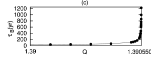
Figure 4: Time interval between bursting oscillations. In all cases, $\alpha=0.037$, $\omega=20.1$, $a=20$. (a) Time between major peaks as a function of the strength coefficient $Q$ for the case of $\xi=0.06$; (b) Variation of the time between major peaks as a function of $Q$ and for different values of $\xi$ from 0.06 to 0.11; (c) The extension to higher values of $Q$ leads to larger time intervals between major peaks for $\xi=0.06$.

Another important feature of the dynamics is the fact that the time interval $\tau_{\rm B}$ between major bursts increases with the strength of the perturbation, as it can be seen in the bottom panels of Figure 2. This is illustrated in Figure 4a, where the time interval between the successive major bursts is shown as a function of the coupling coefficient $Q$. As a visual guide we also plot the shape of the stroboscopic map at the fixed values of $Q$ where an additional inner loop appears. As it can be seen in this panel and in panel 4b, $\tau_{\rm B}$ significantly increases for $Q\in[1.32,1.39]$ whereas for $Q>1.39$ (Figure 4c) the separation between successive bursts increases drammatically. Also, in Figure 4b we show that the above mentioned increase of $\tau_{\rm B}$ can also be obtained by decreasing the non-adiabaticity of the system (that is, decreasing $\xi$). Nevertheless the main parameter for tuning the time interval between major bursts turns out to be $Q$. Note as well that these major bursts favor mass loss at exceptionally high rates and, moreover, the time intervals between them are long. Hence, it is tantalizing to directly connect them with the periodicities observed in the circumstellar shells that can be found surrounding some planetary nebulae (Van Horn et al. 2002).

3.3 Mathematical interpretation of the results

In order to validate the numerical results discussed above, we briefly present the mathematical characteristics of our system. Given that our system is non-autonomous — that is, the Hamiltonian is explicitly time-dependent — the typical methods of analysis of the theory dynamic systems cannot be used. To overcome this drawback, we used an averaging method (Sanders & Verhulst 1985) to transform our system into an autonomous one. The high value of the characteristic frequency ($\omega\gg 1$) assures us that this method is applicable to our case. In the time-averaged framework, the time-dependent perturbation from Eq. (2) becomes $F(r)=-Q\alpha\omega^{4/3}~{}A~{}\sin\omega r$, where $A=-0.04993$ is a constant evaluated numerically. The fixed points of the averaged system in the case of nonzero perturbation must satisfy the conditions:

$$p_{0}=r_{0}^{-4}+Q\alpha\omega^{4/3}A~{}r_{0}^{-2}~{}\sin~{}\omega r_{0}$$ (7)

$$r_{0}^{\beta}p_{0}^{\delta}-1=0~{}.$$ (8)

or, equivalently,

$$G(r)\equiv r^{\beta}(r^{-4}+Q\alpha\omega^{4/3}r^{-2}A~{}\sin~{}\omega r)^{\delta}-1=0.$$ (9)

The roots of Eq. (9) are to be found numerically. The new fixed points of interest are $r_{0}\approx 0.65$ and $r_{0}\approx 1.03$ and represent only slight displacements of the fixed points mentioned before in the case of zero perturbation. Moreover, their associated eigenvalues maintain the form from the previous case (unstable fixed points of saddle-focus type). Increasing the parameter $Q$, a new fixed point is created at about $Q_{0}\approx 1.3855$ at $r\approx 0.86$. This new fixed point is stable as the associated eigenvalues have all negative real parts. With the creation of this fixed point, the looping behaviour dissappears. For higher values of $Q$, the fixed point is replaced by two unstable fixed points again of saddle-focus type. The distance between them increases with $(Q-Q_{0})^{1/2}$. Note, however, that these very high values of $Q$ result in transmissions through the mantle which are not very realistic and, moreover, the time intervals between successive bursts for larger values of $Q$ become very large.

3.4 The role of  $\omega$

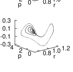
Figure 5: The role of $\omega$. The light curves and the corresponding stroboscopic maps for the cases $\alpha=0.037$, $Q=1.2$ and (top panels) $\omega=10$ ($M=5M_{\odot}$), (middle panels) $\omega=15$ ($M=3M_{\odot}$) and (bottom panels) $\omega=20.1$ ($M=1M_{\odot}$).

Before interpreting the behaviour of the system in the context of real data of stellar variability, we consider worth of interest to explore the role of the parameter $\omega$ and to justify the particular value we have used throughout this work. Icke et al. (1992) concluded that in the case of complete adiabaticity ($\xi=0$), a decrease of $\omega$ leads to stronger chaotic pulsations. The values of $\omega$ used in their work were equivalent to adopting stellar models in the family of low-mass stars ($M\leq 5-8M_{\odot}$) reaching the AGB. In a recent publication (Munteanu et al., 2002), we extended their conclusion to intermediate-mass stars ($8M_{\odot}\leq M\leq 11M_{\odot}$) also in the AGB phase, more precisely to values of $\omega$ around 3. In the previous sections, we have shown that in the case of $\omega=20.1$ a peculiar behaviour is born from the interplay between non-adiabaticity and internal perturbation. Our analysis of the system corresponding to the parametric interval $5\leq\omega\leq 25$ has revealed that such a behaviour is found for values of $\omega$ close to 20, that is for low-mass stars. Mathematically, we attribute this fact entirely to the creation of new fixed points mentioned in the previous section which critically alter the dynamics of the system. They exist for values of $\omega$ higher than about 18. For values slightly lower than 18, the dynamics resembles the one encountered for $\omega=20.1$ (middle panels of Figure 5), but it does not present the successive creation of new loops. Instead, the change of the control parameter $Q$ leads to a mixture of chaotic regimes and uncorrelated creation and dissapearance of new loops. For completeness, we present in Figure 5 the light curves and the stroboscopic maps for three values of $\omega$. For each case, the temporal scaling factor was computed according to the work of Vassiliadis & Wood (1993) which provides a complete set of stellar parameters for AGB stars with initial masses in the range $0.89\leq M/M_{\odot}\leq 5.0$. Due to the richness of the dynamics in the case of $\omega=20.1$, we use it for a comparison with observations.

4 Comparison with observations

The values of the parameters used throughout the numerical integrations were intended to locate the stellar models we are dealing with in the family of Long Period Variables (LPVs) and, specifically, in the families of semiregular and Mira variables. Perhaps the most important of the Mira stars is $o$ Ceti. Its light curve shows a peculiar variability consisting in an exceptional peak occurring every two, three or five “cycles” (Barthés & Mattei 1997). Our simple model naturally recovers this behaviour by tuning the strength of the perturbation or the coupling coefficient. Moreover, we have shown that within our simple model large peaks in the light curve are associated to large inter-pulse intervals.

The Mira stars belonging to the Large Magellanic Cloud constitute the best sample of Miras concerning both periodicities and luminosities. In Figure 6a we show the observational data for some Mira stars in the LMC (Feast 1989) and the best fit to the observational data. Among them, the ones having periods longer than about 400 days clearly appear to be over-luminous with respect to the period-luminosity relationship found for Miras with relatively short periods (Zijlstra et al. 1996; Bedding et al. 1998). With this in mind we have obtained a period-luminosity relationship from our theoretical models using the time interval $\tau_{\rm B}$ and averaged values of the major peaks in luminosity. More precisely, we have varied the parameter $Q$ in the range $[1,1.26]$ resulting in light curves whose major peaks have periodicities (in days) within the range $2.4\la\log\tau_{\rm B}\la 3.0$. The corresponding bolometric magnitudes were computed using a reference value for the equilibrium stellar luminosity of $\log(L_{\star}/L_{\odot})=3.5$ (Vassiliadis & Wood 1993) which is typical for Mira stars. Our theoretical period-luminosity relationship is shown in Figure 6b. For the sake of comparison we also show in this panel all those Miras with $\log P>2.4$ and $M_{\rm bol}<-5.0$, that is all the stars which are found to be over-luminous in Figure 6a. We have also included two other interesting Miras: R Hya and V Hya. As it can be seen our theoretical period-luminosity relationship fits very well the observational data. Moreover, note as well that the observations tend to cluster around fixed regions of the period-luminosity relationship. These regions are coincident with the regions where we find regular oscillations with a fixed number of loops in the stroboscopic map and its sequence of period-doubling cascade leading to chaos. The gaps between the theoretical data are the consequence of the drastic change in the characteristics of our light curves when a new loop is created, and correspond to a very small change of the coupling coefficient. Hence, according to our analysis we should not find almost any star in these regions, which is exactly what it is found.

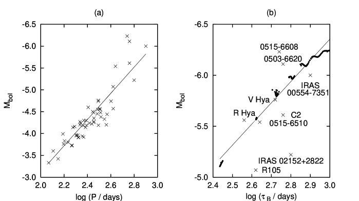
Figure 6: Period-Luminosity relation for Mira stars. (a) PL relation for Mira stars in the LMC and the data on which the relationship is based (Feast 1989). (b) The PL relation using the data furnished by our model (filled circles): the equivalent $M_{\rm bol}$ of the major peaks and the time interval $\tau_{\rm B}$ between them. The values for the parameters used here are $\alpha=0.037$, $\xi=0.06$ and $Q\in[1,1.26]$. The crosses represent a sample of over-luminous Mira stars in the LMC. See text for additional details.

Another peculiarity of Mira stars is that some of them show alternating deep and shallow minima, giving the appearance of double maxima. Some examples are R Cen, R Nor, U CMi, RZ Cyg and RU Cyg — see Hawkins (2001) and references therein. Among these, R Cen has the most persistent and stable double maxima in the light curve while for the rest of the cases the second maximum is often weak and the light curve sometimes reverts to that of a normal Mira. Our simplistic model provides such light curves for small values of the parameter $Q$. As for the general “chaotic connection” for the Mira variables, the first (and unique) case of evidence of chaotic pulsation in a Mira star (R Cyg) comes from the study by Kiss & Szatmáry (2002). They associate the long sub-segments of alternating maxima in R Cyg to a period-doubling event, supporting therefore the well-known scenario of period-doubling to chaos, which we also find in our model. Buchler et al. (2001) present an overview of observational examples of chaotic behaviour in some semiregular variables (SX Her, R UMi, RS Cyg, and V CVn). They argue that AGB stars are prone to chaotic pulsations due to the fact that relative growth rates of the lowest frequency modes are of the order of unity. Higher relative growth rates are a consequence of higher luminosity–mass ratios, that is more non-adiabatic stars. Hence, not only semiregular variables, but also Mira stars should also be candidates for chaotic pulsators. In spite of its simplicity, our toy-model presents chaotic pulsations for certain intervals of the parameters characterizing the strength of the internal driving and, thus, could provide some support to the conjecture that the evolution of semiregulars and of Mira stars is strongly connected.

5 Conclusions and caveats

We have introduced a weakly non-adiabatic one-zone model driven by sinusoidal pressure waves intended to reproduce the irregular pulsations of Mira-like variables for which other simple models already exist (Buchler & Regev 1982; Auvergne & Baglin 1985; Reid & Goldston 2002). Our model extends the works of Icke et al. (1992) and Saitou et al. (1989). In particular, Icke et al. (1992) proposed an adiabatic model driven by pressure waves (the piston approximation) whereas Saitou et al. (1989) studied a simple non-adiabatic model without driving (the self-excited pulsation model). Our approach is justified by the large density contrast between the interior and the outer layers. One-zone models have limitations since some Mira stars are suspected to have at least two frequencies (Mantegazza 1996) which may vary independently, suggesting that more than one mode is involved. Clearly, one-zone models are unable to reproduce this behaviour. Nevertheless, the majority of Miras do not show this behaviour. Another interesting approach would have been to use the modal coupling. However, although this approach has been used to model the pulsation of Miras (Buchler & Goupil 1988), it is more appropriate for classical Cepheids, RR Lyrae and W Vir stars — see Buchler et al. (1993) and references therein. It is also worth noting here that the piston approximation — first introduced by Bowen (1988) — used in this paper has been used since then by several authors (Fleischer et al. 1995; Höfner et al. 2003) even if it has never been deeply scrutinized for validity. Nevertheless this approximation appears to correctly reproduce the velocities and mass loss rates typical of AGB stars. Hence, this approximation can be regarded as a reasonable first-order approximation of the dynamical effect of the pulsation on the atmosphere. To summarize, our model should be considered as a toy model that qualitatively reproduces the general features of the light curves.

We have thoroughly explored the interesting particularities of the system from both the astrophysical and from the mathematical points of view. We have found that the degree of non-adiabaticity turns out to be a determining factor in the development of the period-doubling route to chaos. As far as the transition to chaos is concerned, an increase in the degree of non-adiabaticity plays the same role as a decrease of the effective temperature in the model studied by Saitou et al. (1989). Moreover, due to the time-dependent perturbation, a knot-like structure is created in the phase space when varying the transmission coefficient ($Q$) while the strength of the perturbation is kept fixed. The resulting periodic light curves are characterized by a repetitive pattern consisting in a major peak followed by $n$ minor peaks, where $n$ is given by the number of loops in the phase space. Our theoretical light curves are in qualitative agreement with those of several well-known Mira stars. In particular the prototype of Mira stars, $o$ Ceti, shows this pattern of alternating major peaks followed by several minor peaks. Furthermore, for a given choice of our input parameters the resulting light curves also resemble those of some peculiar Miras (R Cen, R Nor, U CMi, RZ Cyg, or RU Cyg) which appear to have double maxima due to alternating deep and shallow minima. We have found as well that our dynamical system presents both chaotic regimes and patterns of periodicity. The chaotic regions occur for ranges of $Q$ between those corresponding to the creation of a new luminosity peak between major bursts. We have also noticed that for increasing strengths of the perturbation the time interval between major bursts increases. This interval increases with $Q$ as well. At high values of the strength of the perturbation within the range yielding the knot-like structure, we obtained a peculiar behaviour: the creation of new loops stops and the resulting light curves show a time interval during which the luminosity preceeding every major peak remains constant.

We have also obtained a theoretical period-luminosity relationship and compared it with the observational data of Miras in the LMC. In particular, we have focused on those peculiar Miras with long periods which are known to be over-luminous with respect to the best fit of Feast (1989). We have found that our model provides a reasonable fit to the period-luminosity relationship of these stars and also to the observed clustering of the over-luminous stars around certain regions in the period-luminosity diagram. The ultimate reason for this fact is closely related to the creation of a new loop in the stroboscopic map, and, consequently, of a new luminosity peak in the corresponding time series.

Finally, we would like to stress that although our simple model succeeds in furnishing reasonable comparisons with real data, a detailed quantitative interpretation is beyond its capabilities because of its crude physical assumptions. In particular, next steps towards improving the one-zone approach could eventually include the treatment of convection which is supposed to play an important role in the envelopes of these stars. This improvement will affect also the functional form of the luminosity which was rather simplified in the present work.

Acknowledgements. This work has been supported by the MCYT grant AYA2000–1785, by the MCYT/DAAD grant HA2000–0038 and by the CIRIT grants 1995SGR-0602 and 2000ACES-00017. We would also like to acknowledge our anonymous referee for valuable criticisms and suggestions.

References

- [1] Aikawa, T., 1987, Ap. & Space Sci., 139, 281
- [2] Aikawa, T., 1990, Ap. & Space Sci., 164, 295
- [3] Auvergne, M., Baglin, A., 1985, A&A, 142, 388
- [4] Baker, N.H., Moore, D.W., Spiegel, E.A., 1966, AJ, 71, 844
- [5] Barthès, D., Mattei, J.A., 1997, AJ, 113, 373
- [6] Bedding, T.R., Zijlstra, A.A., Jones, A., Foster, G., 1998, MNRAS, 301, 1073
- [7] Buchler, J.R., Goupil, M.J., Kóvacs, G., 1987, Phys. Lett. A, 126, 177
- [8] Buchler, J.R., 1993, Ap. & Space Sci., 210, 9
- [9] Buchler, J.R., Kóvacs, G.,1987, ApJ, 320, L57
- [10] Buchler,J.R., Kolláth, Z., Cadmus, R., 2001, in Experimental Chaos, AIP Conference Proc. 622, 61
- [11] Buchler, J.R., Regev, O., 1982, ApJ, 263, 312
- [12] Buchler, J.R., Goupil, M.J., 1988, A&A, 190, 137
- [13] Feast, M.W., 1989, MNRAS, 241, 375
- [14] Fleischer, A.J., Gauger, A., Sedlmayr, E.,1995, A&A, 297, 543
- [15] Gautschy, A., Glatzel, W., 1990, MNRAS, 245, 597
- [16] Gautschy, A., Saio, H., 1995, ARA&A, 33, 113
- [17] Groenewegen, M.A.T., de Jong,T., 1994, A&A, 288, 782
- [18] Habing, H.J., 1996, A&AR, 7, 97
- [19] Hawkins, G., Mattei, J.A., Foster, G., 2001, PASP, 113, 501
- [20] Höfner, S., Gautschy-Loidl, R., Aringer, B., 2003, A&A, in press
- [21] Icke, V., Frank, A., Heske, A., 1992, A&A, 258, 341
- [22] Kiss, L.L., Szatmáry, K., 2002, A&A, 390, 585
- [23] Kóvacs, G., Buchler, J.R., 1988, ApJ, 334, 971
- [24] Mantegazza, L., 1996, A&A, 315, 481
- [25] Munteanu, A., García–Berro, E., José, J., Petrisor, E., 2002, Chaos, 12, 332
- [26] Reid, M.J., Goldston, J.E., 2002, ApJ, 568, 931
- [27] Saitou, M., Takeuti, M., Tanaka, Y., 1989, PASP, 41, 297
- [28] Stellingwerf, R.F., 1972, A&A, 21, 91
- [29] Stellingwerf, R.F., 1986, ApJ, 303, 119
- [30] Tanaka, Y., Takeuti, M., 1988, Ap. & Space Sci., 148, 229
- [31] Vassiliadis, E., Wood, P.R., 1993, ApJ, 413, 641
- [32] Willson, L.A., 2000, ARA&A, 38, 573
- [33] Wood, P.R., 2003, in press, in Mass-losing Pulsating Stars and their Circumstellar Matter, Eds.: Y. Nakada & M. Honma (Kluwer: Dordrecht)
- [34] Zijlstra, A.A., Loup, C., Walters, L.B., Whitelock, F.M., van Loon, J.T., Gugliemo, F., 1996, MNRAS, 279, 32