The Formation of a Disk Galaxy
within a Growing Dark Halo

We present a dynamical model for the formation and evolution of a massive disk galaxy, within a growing dark halo whose mass evolves according to cosmological simulations of structure formation. The galactic evolution is simulated with a new three-dimensional chemo-dynamical code, including dark matter, stars and a multi-phase ISM. The simulations start at redshift $z=4.85$ with a small dark halo in a $\Lambda$CDM universe and we follow the evolution until the present epoch. The energy release by massive stars and supernovae prevents a rapid collapse of the baryonic matter and delays the maximum star formation until redshift $z\approx 1$. The metal enrichment history in this model is broadly consistent with the evolution of [Zn/H] in damped Ly$\alpha$ systems. The galaxy forms radially from inside-out and vertically from halo to disk. As a function of metallicity, we have described a sequence of populations, reminiscent of the extreme halo, inner halo, metal-poor thick disk, thick disk, thin disk and inner bulge in the Milky Way. The first galactic component that forms is the halo, followed by the bulge, the disk-halo transition region, and the disk. At redshift $z\approx 1$, a bar begins to form which later turns into a triaxial bulge. Despite the still idealized model, the final galaxy resembles present-day disk galaxies in many aspects. The bulge in the model consists of at least two stellar subpopulations, an early collapse population and a population that formed later in the bar. The initial metallicity gradients in the disk are later smoothed out by large scale gas motions induced by the bar. There is a pronounced deficiency of low-metallicity disk stars due to pre-enrichment of the disk ISM with metal-rich gas from the bulge and inner disk (”G-dwarf problem”). The mean rotation and the distribution of orbital eccentricities for all stars as a function of metallicity are not very different from those observed in the solar neighbourhood, showing that early homogeneous collapse models are oversimplified. The approach presented here provides a detailed description of the formation and evolution of an isolated disk galaxy in a $\Lambda$CDM universe, yielding new information about the kinematical and chemical history of the stars and the interstellar medium, but also about the evolution of the luminosity, the colours and the morphology of disk galaxies with redshift.

1 Introduction

During the last decade, significant progress has been made in understanding cosmic structure formation and galactic evolution. With high-resolution cosmological simulations, the formation of dark halos in different cosmologies has been studied in detail (e.g.  Navarro et al., 1996; Moore et al., 1998; Colín et al., 2000; Yoshida et al., 2000; Avila-Reese et al., 2001; Jenkins et al., 2001; Klypin et al., 2001) to determine the large-scale mass distribution, the halo merging histories, the structural parameters of the dark halos, and finally the formation of galaxies inside these dark halos (Steinmetz & Müller, 1995; Kay et al., 2000; Navarro & Steinmetz, 2000b; Mosconi et al., 2001; Pearce et al., 2001).

In many respects, these simulations are in agreement with observations, but there remain a number of difficulties. Firstly, the universal cuspy halo density profiles (Navarro et al., 1997; Moore et al., 1999; Fukushige & Makino, 2001), while in agreement with observations of galaxy clusters, are in apparent disagreement with the flat dark matter density distributions inferred from observations in the centres of galaxies (Salucci & Burkert, 2000; Blais-Ouellette et al., 2001; Borriello & Salucci, 2001; de Blok et al., 2001). Secondly, the specific angular momenta and scale lengths of the disk galaxies in the cosmological simulations are too small compared to real galaxies (Navarro & Steinmetz, 2000b). This may be partially a numerical problem of SPH simulations, but is more likely due to overly efficient cooling and strong angular momentum transport from the baryons to the dark halos during merger events (Navarro & Benz, 1991). Thacker & Couchman (2001) and also Sommer-Larsen et al. (1999) showed the angular momentum problem in CDM simulations may be resolved by the inclusion of feedback processes. Thirdly, the cold dark matter (CDM) simulations predict a large number of satellite galaxies in the neighbourhood of giant galaxies like the Milky Way Galaxy, but this is not observed (Moore et al., 1999).

The cosmological simulations are used to describe the large-scale evolution of the dark matter distribution from the primordial density fluctuations to the time when the dark halos form. It is inevitable in such simulations that structures on galactic and sub-galactic scales are not well-resolved. Furthermore, it is difficult to incorporate the detailed physics of the baryonic component, that is of the multi-phase interstellar medium (ISM), and the feedback processes between stars and ISM. These are serious drawbacks, because feedback from stars can prevent a proto-galactic cloud from rapid collapse and it can trigger large scale gas motions (Samland et al., 1997). Both alter the galactic formation process significantly.

Complementary ways to circumvent at least some of these problems are (i) to combine the large-scale simulations with semi-analytical galaxy models (Guiderdoni et al., 1998; Somerville & Primack, 1999; Boissier & Prantzos, 2000; Cole et al., 2000; Kauffmann & Haehnelt, 2000), or (ii) to simulate the formation of only single galaxies or small galactic groups using either cosmological initial conditions or a simplified, but cosmologically motivated model of the dark matter background (Navarro & Steinmetz, 1997; Berczik, 1999; Hultman & Pharasyn, 1999; Sommer-Larsen et al., 1999; Bekki & Chiba, 2001; Thacker & Couchman, 2001; Williams & Nelson, 2001). While the semi-analytical models are advantageous for investigating the global properties of galaxy samples, the small-scale dynamical models provide information about the detailed structure of galaxies, the kinematics of the stellar populations and the ISM, and the star formation histories. The dynamical models are called chemo-dynamical (Theis et al., 1992; Samland et al., 1997; Bekki & Shioya, 1998; Berczik, 1999; Williams & Nelson, 2001), if they include different stellar populations, a multi-phase ISM, and an interaction network that describes the mass, momentum and energy transfer between these components.

The aim of the present work is to investigate how a large disk galaxy forms inside a growing dark halo in a realistic $\Lambda$CDM cosmogony. We present the results of a new three-dimensional model, including dark matter, stars, and a multi-phase ISM. The mass infall at the boundaries of the simulated volume is taken from cosmological simulations (see VIRGO-GIF-project; Kauffmann et al., 1999). We use a total dark matter mass of $1.5\times 10^{12}\mathrm{\,M}_{\sun}$, a total baryonic mass of $3\times 10^{11}\mathrm{\,M}_{\sun}$, a spin parameter $\lambda=0.05$, and an angular momentum profile similar to the universal profile found by Bullock et al. (2001). Different from Bekki & Shioya (1998); Berczik (1999) and Williams & Nelson (2001), we use an Eulerian grid-code for the ISM, which we believe is better suited to describe the multi-phase structure of the ISM and the feedback processes, especially in low-density regions. The final galaxy model provides densities, velocities, velocity dispersions, chemical abundances, and ages for 614 500 stellar particles, and temperatures, chemical abundances, densities, velocities, and pressures of the ISM. The goal of the project is a self-consistent model for the formation and evolution of large disk galaxies, which can be used to understand observations of young galaxies as well as data on stellar populations in the Milky Way.

The paper is organized as follows. Section 2 summarizes some observational material relating to the formation and evolution of galaxies. Section 3 describes our multi-phase ISM model and the underlying dark matter halo model. In Section 4 we outline the formation history of the model disk galaxy. The properties of the galactic halo, bulge and disk components are discussed in Section 5. A summary and a short outlook conclude the paper (Section 6).

2 Observations of the galaxy formation process

Galaxy evolution models can give a simplified description of the evolution of real galaxies and can make predictions that can be tested by observations. The high redshift observations show that the first proto-galactic structures form at redshift $z>3$ (e.g.  Clements & Couch, 1996; Dey et al., 1998; Steidel et al., 1999; Manning et al., 2000). Surveys of high redshift galaxies reveal a wide range of galactic morphologies with considerable substructure and clumpiness (Pentericci et al., 2001). At redshift $z\approx 1-2$, the formation of galactic components (spheroids, halos, bulges and disks) seems to take place (Lilly et al., 1998; Kajisawa & Yamada, 2001). However, the spatial resolution of these high and intermediate redshift surveys (e.g.  Abraham et al., 1999; van den Bergh et al., 2000; Ellis et al., 2001; Menanteau et al., 2001) is still too low to measure more than global galactic properties (e.g.  asymmetry and concentration parameters). There are indications that most of the massive galaxies form before or around $z=1$ (Brinchmann & Ellis, 2000), and especially that the giant ellipticals form at redshifts $z>1$ (Best et al., 1998), (but see van Dokkum et al., 1999), but not before $z=2.4$ (Pentericci et al., 2001). There is a general trend of early type galaxies being older and having higher peak star formation rates than late type galaxies (Sandage, 1986). These general star formation histories seem to be overlapped with star formation bursts, triggered by infalling material or interactions with other galaxies.

Since we can observe galactic sub-structures down to the stellar scale only in our Galaxy, the Milky Way observations are a cornerstone for the understanding of the formation and evolution of all spiral galaxies. From studies of Galactic stars we know that the halo is old and that the disk and bulge contain a mixture of old and young stars. This raises the question in what sequence the galactic components halo, bulge and disk formed, and what was the star formation history. Determinations of the star formation history of the Milky Way and other nearby galaxies were attempted by Bell et al. (2000); Hernandez et al. (2000) and Rocha-Pinto et al. (2000), based on star counts, broad band colours, or chemical compositions of stars.

The chemical and kinematical data from galactic halo stars have been one of the starting points for different scenarios for the formation and evolution of galaxies. Eggen et al. (1962) were the first to propose a monolithic collapse galactic formation model in which the Milky Way forms rapidly out of a collapsing proto-galactic cloud. This was based on data for galactic halo stars which are now known to have been plagued by selection effects (Chiba & Beers, 2000). Later, based on observations of halo globular clusters, Searle & Zinn (1978) proposed a new model in which the Milky Way forms out of merging lumps and fragments which all have their individual star formation histories. The contrasting nature of these two models and the proposed observable differences (e.g.  existence or non-existence of metallicity gradients, the expected age spread for halo objects) seemed to offer a simple way to deduce the formation history of disk galaxies from Milky Way observations. However, new data especially from proper motion catalogues, lead to the conclusion that at least the halo of the Milky Way formed neither by a monolithic collapse nor by a pure merging process (Sandage, 1990; Unavane et al., 1996; Chiba & Beers, 2000). In the modern hybrid scenarios, a part of the Galactic halo formed during a dissipative process (collapse) and another part shows signatures of merging events. For example, Chiba & Beers (2000) proposed a scenario in which “the outer halo is made up from merging and/or accretion of sub-galactic objects, such as dwarf-type satellite galaxies, whereas the inner part of the halo has undergone a dissipative contraction on relatively short time scales”. This is consistent with the findings of Helmi et al. (1999), who found that 10% of the metal-poor stars in the outer halo of the Milky Way are aligned in a single coherent structure, which they identify as the remnant of a disrupted dwarf galaxy. These hybrid scenarios are, in the general outline, also consistent with the formation of galaxies in a hierarchical universe (Chiba & Beers, 2000).

3 The model

The formation and evolution of a galaxy is influenced by the cosmological initial conditions and the environment, but also by internal feedback processes. Heating by supernovae (SNe), dissipation, radiative cooling, as well as in- and outflows influence the evolution both locally and globally. Our new three-dimensional galactic model takes into account the dynamics of stars and the different phases of the ISM, as well as the processes (“chemistry”) which connect the ISM and the stars. These baryonic components are embedded in a collision-free dark matter halo taken from simulations of cosmological structure formation. The description of the ISM is based on that used in the two-dimensional chemo-dynamical models of Samland & Hensler (1996); Samland et al. (1997). The following subsections contain a brief outline of our model.

3.1 The dark halo

Cosmological simulations (e.g.  Navarro et al., 1995; Moore et al., 1999; Pearce et al., 1999) show that in a hierarchical universe galaxies form out of a few large fragments with an additional slow accretion of mass. Thus each galaxy has its own formation history and characteristic shape, depending on the masses, angular momenta and merging histories of the fragments. Yet the formation of the CDM halos can be described by some simple ”universal” formulae. Wechsler et al. (2002) and van den Bosch (2002) calculated the mass accretion history, Bullock et al. (2001) the angular momentum distribution, Navarro et al. (1997) and others the density profiles and Del Popolo (2001) and Wechsler et al. (2002) the evolution of the concentration parameter.

3.1.1 The dark matter halo formation history

In the hierarchical formation scenario, a dark halo may form early and rapidly or grow slowly with time. For the model described in this paper we take an average halo formation history, because at present we cannot simulate the evolution of a galaxy for a large number of different halo formation histories. We choose a $\Lambda$CDM universe with $\Lambda=0.7$, $\Omega=0.3$, a Hubble constant $h_{0}=0.7$ and a baryonic-to-dark matter ratio of 1:5. From the cosmological N-body simulations of the VIRGO-GIF-project (Kauffmann et al., 1999), we extracted the merging trees of 96 halos, all with a final mass of $1.8\times 10^{12}\mathrm{\,M}_{\sun}$. Figure 1 shows the average halo mass growth, which is in agreement with the universal mass accretion histories found by van den Bosch (2002) and Wechsler et al. (2002). The individual merging histories can be quite different; two extreme cases with early and late mass growth are shown in the small panels at the top left and right of Fig. 1.

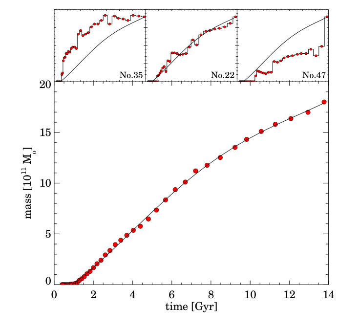
Figure 1: The dots shows the average mass from 96 different halo merging trees, which all result in a $1.8\times 10^{12}\mathrm{\,M}_{\sun}$ halo. The smooth line shows the approximation which is used in our numerical model. The most extreme halo merging trees and that which shows the smallest deviations from the average are shown in the smaller upper panels. Data from the VIRGO-GIF-project (Kauffmann et al., 1999)

We assume that the growing dark halo has the universal density profile as proposed by Navarro et al. (1997), and that its mass is accreted in spherical shells. Given the current halo mass and the evolution of the critical density, we can determine the outer halo radius $r_{200}$ (see Mo et al., 1998). A free parameter that remains is the mass concentration $c$, which in the present simulation is assumed to be $c=9.2$. At redshift $z=0$, this leads to a circular velocity of $v_{\mathrm{circ}}=179\mathrm{\,km\,s^{-1}}$ at the $r_{200}=250\mathrm{\,kpc}$ radius. Inside a galactocentric radius of $8.5\mathrm{\,kpc}$, the final mass of dark matter is $4\times 10^{10}\mathrm{\,M}_{\sun}$, comparable to the upper limit of the dark matter content inside the solar circle ($5.2\times 10^{10}\mathrm{\,M}_{\sun}$; Navarro & Steinmetz, 2000a).

Treating the growing dark matter halo as a spherical background potential that does not respond to the baryonic component minimizes gravitational torques during the collapse and thereby circumvents the well-known angular momentum problem (Navarro & Steinmetz, 2000b). The accretion in this model is smoother as compared to hierarchical models, where a fraction of the mass accretion takes place through merging dark matter fragments, unless the gas in these hierarchical fragments is dispersed by early star formation and feedback.

3.1.2 The angular momentum of the dark matter

During the hierarchical clustering, tidal torques induce shear flows which lead to rotating proto-galactic systems. N-body simulations show that, independent of the initial perturbation spectrum and the cosmological model, the spin parameter of the dark halos is in the range $\lambda=L|E|^{0.5}G^{-1}M^{-2.5}=0.02-0.11$ with an average value of $\lambda=0.04-0.05$ (Barnes & Efstathiou, 1987; Steinmetz & Bartelmann, 1995; Cole & Lacey, 1996; van den Bosch, 1998; Gardner, 2001).

Bullock et al. (2001) studied the angular momentum profiles of dark halos in a $\Lambda$CDM cosmology. They found that the spatial distribution of the angular momentum in most of the halos show a certain degree of cylindrical symmetry, but that a spherically symmetric angular momentum distribution with a power-law $j(r)\propto r^{1.1\pm 0.3}$ is also a good approximation. We consider the following two rotation fields for the halo:

$$v_{rot}^{halo}=v_{0}{\sqrt{x^{2}+y^{2}}\over\sqrt{x^{2}+y^{2}+z^{2}}+d_{0}}\equiv v_{0}{|r|\over|d|+d_{0}}$$ (1)

$$v_{rot}^{halo}=v_{0}{\sqrt{x^{2}+y^{2}}\over\sqrt{x^{2}+y^{2}}+d_{0}}\equiv v_{0}{|r|\over|r|+d_{0}}$$ (2)

$v_{0}$ and $d_{0}$ are constants which determine the total amount of angular momentum and the rotation curve near the rotation axis, respectively.

Assuming that initially the mass and velocity distributions of the baryonic matter coincide with those of the dark matter, and that baryonic mass and specific angular momentum is conserved during the collapse to a disk (Mestel, 1963; Fall & Efstathiou, 1980), we can estimate the disk surface density profiles corresponding to these rotation fields. Figure 2 shows the results, calculated for collapse in the pure NFW potential. As already pointed out by Fall & Efstathiou (1980), disks with exponential surface density profiles are found when the halo has a rising rotation curve at small radii and a nearly constant rotation velocity in the outer parts. In the present case, the cylindrical halo rotation model (eqn. 2) also produces an exponential disk, at least in the inner $20\mathrm{\,kpc}$. The spherical rotation model (eqn.1) instead leads to higher surface densities near the galactic centre which favours the formation of a bulge. In the following we use the spherical rotation model with a spin parameter $\lambda=0.05$, to fix the initial angular momentum distribution of the baryonic matter.

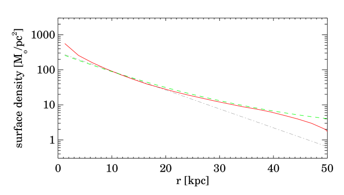
Figure 2: Surface density of the galactic disk if the specific angular momentum is conserved during the proto-galactic collapse in our NFW halo model. The cylindrical rotation leads to an exponential disk in the inner $20\mathrm{\,kpc}$ (dashed curve), while the spherical rotation produces an exponential disk with an additional mass at the centre (full line). The thin dash-dotted line shows an exponential disk with a scale length of $8\mathrm{\,kpc}$.

3.2 The Stars

The stellar motions have a considerable influence on the galactic evolution, since the time-delayed stellar mass loss and energy release connect different regions and also different galactic evolution phases. The approximately $10^{11}$ stars in a large galaxy form a collision-less system. Each star moves on its own orbit, which is determined by the conditions under which the star formed and the evolution of the galactic gravitational potential. We use a particle-mesh method (Hockney & Eastwood, 1988), in which the passing of the stellar particles to the mesh and also the interpolation of the gravitational forces at the particle positions is done with a cloud-in-cell method. This method is fast and second order accurate, but it is limited by the spatial resolution of the underlying grid, which at present is $370\mathrm{\,pc}$.

Each stellar particle represents an ensemble of stars with a stellar mass function. In the present model, we assume a Salpeter initial mass function (IMF) with lower and upper mass limits of $0.8\mathrm{\,M}_{\sun}$ and $50\mathrm{\,M}_{\sun}$, and with an additional lock-up mass fraction of 60%. The lock-up mass equals the mass of all stars below $0.8\mathrm{\,M}_{\sun}$. During a simulation the star formation rate is calculated on the spatial grid, and in timesteps of $10\mathrm{\,Myr}$ representative samples of 500 new stellar particles are created. This yields 614 500 particles at the end of the simulation. Depending on the star formation rate a single particle represents $10^{4}$ to $10^{7}$ stars. The initial chemical composition and velocity of a stellar particle is derived from the chemical composition, velocity and velocity dispersion of the parent molecular cloud medium.

We assume that the evolution of the stars is determined only by their initial mass and metallicity, neglecting effects of stellar rotation or star-star interactions. From the stellar evolution models of Maeder & Meynet (1989); Schaller et al. (1992) and Schaerer et al. (1993) we get the lifetimes, energy releases and mass losses on the main sequence. We can subdivide stars into three main classes.

First, the low mass stars which stay on the main sequence during the whole galactic evolution. These stars become noticeable only by their gravitational forces and because they lock-up a major fraction of the galactic mass. The total lock-up mass has influence on the galactic gas content and therefore on the sequence of stellar generations. It is important in smaller galaxies where SN-driven winds reduce the mass in gas, but not the mass locked up in low mass stars.

The second class of stars are intermediate in mass. When they leave the main sequence, they loose a substantial fraction of the initial mass (asymptotic giant branch and planetary nebula phase); however, the energy release of these stars is small compared to other energy sources.

The third class of stars are the massive stars, typically with masses in excess of $8-10\mathrm{\,M}_{\sun}$. These stars are a major source of both energy and mass return in a galaxy. The UV-radiation and the kinetic energy release during the final explosion (SN type II) ionize and accelerate the ISM. This can trigger large-scale gas flows and star formation which both influence the galactic evolution.

A rare but important galactic event is the explosion of SNe of type Ia. The most probable progenitor candidates are close binary stars consisting of a white dwarf and a main sequence star. We include this process, since it is a major source of iron peak elements (Nomoto et al., 1984).

3.3 The Interstellar Medium

The ISM in galaxies exists at different densities and temperatures, and it shows phase transitions on short timescales compared to the age of a galaxy. In the present galactic model we use a simplified ISM description based on the three-phase model of McKee & Ostriker (1977). The three phases are a cold, a warm and a hot phase, with typical temperatures of $80\mathrm{\,K}$, $8000\mathrm{\,K}$ and $10^{6}\mathrm{\,K}$, respectively. The cold phase is found in the dense cores of molecular clouds. These cores are embedded in warm neutral or ionized gas envelopes. Outside the clouds the space is filled with hot, dilute gas. The three-phase model is a simplification, but it is realistic enough to use it in a global galactic model. A critical discussion of the weak and strong points of the three-phase model can be found in McKee (1990).

Essentially, the temperatures and densities of the ISM phases determine most of the physical processes in the ISM. However, the geometry of the clouds is also important for processes that take place in the phase transition regions (e.g. evaporation and condensation) or that depend on the sizes of the clouds explicitly (e.g. cloud-cloud collisions and star formation). In our model, we assume spherical clouds which follow the mass-radius relation of Elmegreen (1989)

$${M\over R^{2}}=190\left({\mathrm{\,M}_{\sun}\over\mathrm{\,pc}^{2}}\right)\sqrt{P_{4}}.$$ (3)

$P_{4}={P_{\mathrm{e}}/\mathrm{k}\over 10^{4}\mathrm{K}/\mathrm{cm}^{3}}$ is the pressure in the ambient ISM. The mean cloud mass is $10^{5}\mathrm{\,M}_{\sun}$; this is derived from the cloud mass spectrum of Dame et al. (1986) for star forming giant molecular clouds in the mass range of $10^{4}\mathrm{\,M}_{\sun}$ to $10^{6}\mathrm{\,M}_{\sun}$.

In the present dynamical description, we use only a two-phase model for the ISM, containing hot gas with embedded (cold+warm) clouds. The motions of both components are described by the time-dependent hydrodynamical equations (mass, momentum and energy conservation). Similar as in the two-dimensional chemo-dynamical models (Samland et al., 1997) we use a fractional step method to split the problem into source, sink and transport steps. The problem of the three-dimensional transport is broken down into a number of one-dimensional problems for the densities, metallicities, momenta and energies (dimensional splitting). Using the van Leer advection scheme (van Leer, 1977) combined with the consistent advection method (Norman et al., 1980) and the Strang splitting (Strang, 1968), the advection is second order accurate. In the Strang splitting the three-dimensional transport is split into a sequence of five one-dimensional transport steps:

$$\Delta t\@vec{A}=({\Delta t\over 2}\@vec{A_{x}})({\Delta t\over 2}\@vec{A_{y}})(\Delta t\@vec{A_{z}})({\Delta t\over 2}\@vec{A_{y}})({\Delta t\over 2}\@vec{A_{x}})$$ (4)

where $\Delta t$ is the time step length, $\@vec{A_{x}}$, $\@vec{A_{y}}$, $\@vec{A_{z}}$ are the differential operators which describe the transport in $x$, $y$, $z$ direction, and $\@vec{A}$ is the operator for the three-dimensional problem. Approximately the same accuracy can be achieved by a simpler splitting scheme which uses an alternating sequence of only three one-dimensional transport steps:

$$(\Delta t\@vec{A})(\Delta t\@vec{A})=\left[(\Delta t\@vec{A_{x}})(\Delta t\@vec{A_{y}})(\Delta t\@vec{A_{z}})\right]$$

$$\left[(\Delta t\@vec{A_{z}})(\Delta t\@vec{A_{y}})(\Delta t\@vec{A_{x}})\right]$$ (5)

For the $\sim 10^{6}$ transport steps in our galactic evolution simulations, both splitting schemes lead to identical results. However, the second method is faster by a factor of 1.6.

3.4 The interaction network

The interactions between stars and ISM are very important for the galactic evolution. They determine the evolution timescale of a galaxy to a large extent. In the following subsections we give a short overview about the processes which we take into account, and discuss the influence of the free parameters in the parametrization of these processes.

3.4.1 Star formation

Star formation is obviously one of the most important processes during the galactic evolution, but it is one of the least understood. Early on, Schmidt (1959) found that the star formation rate in the solar neighbourhood varies with the square of the surface gas density $\Sigma_{\mathrm{gas}}$ of the ISM. More recently, Kennicutt (1998) found a star formation rate for disk and starburst galaxies which is proportional to $\Sigma_{\mathrm{gas}}^{1.4\pm 0.15}$, with a sharp decline below a critical surface density threshold ($\approx 3$-$13\mathrm{\,M_{\odot}\,pc^{-2}}$). Remarkably, this simple law describes star formation in galaxies for which the average gas consumption time can vary from $3\cdot 10^{8}\mathrm{\,yr}$ (starbursts) to $2\cdot 10^{9}\mathrm{\,yr}$ (normal disks).

Motivated by these findings we use the following star formation law:

$$\dot{\rho}_{\mathrm{sf}}={\rho_{\mathrm{cld}}\over t_{\mathrm{sf}}}={\rho_{\mathrm{cld}}\over c_{\mathrm{sf}}t_{\mathrm{dyn}}}$$ (6)

Here $\rho_{\mathrm{cld}}$ is the average density of the cloudy medium, $t_{\mathrm{sf}}$ the star formation timescale, and $t_{\mathrm{dyn}}$ the dynamical timescale for the average star forming cloud mass. For the cloud model described in Section 3.3 the dynamical timescale of the average star forming cloud is

$$t_{\mathrm{dyn}}=\sqrt{3\pi\over 32G\hat{\rho}_{\mathrm{cld}}}=16.2\cdot P_{4}^{-3/8}.$$ (7)

Molecular clouds do not collapse and form stars on a single dynamical timescale, because magnetic fields or turbulent motions stabilize the clouds. To account for these processes, we include the factor $c_{\mathrm{sf}}$. If we take into account that a part of the clouds is only confined by pressure and that the timescales for ambipolar diffusion and dissipation of turbulent energy are much longer than the dynamical timescale, we expect $c_{\mathrm{sf}}\gg 1$. $c_{\mathrm{sf}}$ can be estimated from the observed number of OB stars in the solar neighbourhood (Reed, 2001). Assuming that the stellar mass function follows a Salpeter law with lower and upper mass limits of $0.1\mathrm{\,M}_{\sun}$ and $50\mathrm{\,M}_{\sun}$, we derive a local star formation rate of $1.8\times 10^{-5}\mathrm{\,M_{\odot}\,pc^{-3}\,Myr^{-1}}$. From the local ISM density and pressure ($\rho\approx 0.035\mathrm{\,M_{\odot}\,pc^{-3}}\approx 1\mathrm{\,cm^{-3}}$, $P_{4}\approx 1$), we find $c_{\mathrm{sf}}=120$, which means that the on average the star formation timescale exceeds the dynamical timescale by factor of 120. The final star formation law can then be written as

$$\dot{\rho}_{\mathrm{sf}}=\eta_{\mathrm{sf}}\rho_{\mathrm{cld}}P_{4}^{3/8}$$ (8)

with a star formation (gas depletion) timescale $t_{\mathrm{sf}}\approx 1/\eta_{\mathrm{sf}}=1.9\mathrm{\,Gyr}$ in the local Galactic disk. The star formation rate is proportional to $\rho_{\mathrm{cld}}^{1.375}$ if the cloudy medium is in pressure equilibrium ($P_{4}\propto\rho_{\mathrm{cld}}$). This is the quiescent star formation mode in the model. During the collapse or if large fragments merge, the pressure can increase and the star formation can be more efficient.

Figure 3 shows the resulting star formation rate as a function of the surface density of gas, in the forming disk galaxy model described in Section 4. Both the average star formation rates and the star formation rates in the strongest star formation regions are slightly higher than, but consistent with Kennicutt’s 1998 data and mean relation, over a range of surface densities extending from normal disk galaxies into the starburst galaxy region. Had we calibrated the factor $\eta_{\mathrm{sf}}$ on Kennicutt’s diagram, the resulting value would have been about a factor of 2 smaller than that based on the solar neighbourhood OB stars. The typical scatter in Kennicutt’s plot corresponds to a factor of 2.2 dispersion in $\eta_{\mathrm{sf}}$.

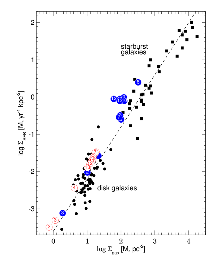
Figure 3: Star formation rate in the forming disk galaxy model described in Section 4, versus the projected surface density of the cloudy medium in a $20\mathrm{\,kpc}$ sphere. Open numbered circles are for average star formation rates and surface densities within $20\mathrm{\,kpc}$; the number denotes the galactic age in Gyr. The filled numbered circles are for the most prominent star formation region at the same galactic ages. The black dots and black squares denote the data from Kennicutt (1998) for disk galaxies and starburst galaxies. The dashed line is Kennicutt’s mean relation.

3.4.2 Massive stars and supernovae type II

Massive stars and SNe influence the galactic evolution in several ways. They heat the ISM, produce shells and filaments and stir up the cloudy medium. In addition, they are the most important source of heavy elements and they determine the chemical evolution of a galaxy. The lifetimes of the massive stars range from 3 to $30\mathrm{\,Myr}$ before they finally explode as SNe II. Only a stellar remnant of $\approx 2\mathrm{\,M}_{\sun}$ remains. The rest of the mass is blown away by stellar winds or expelled during the explosion. On average a massive star on the main sequence emits about $6\times 10^{51}\mathrm{\,erg}$ in photons (Schaerer & Vacca, 1998) which ionize the surrounding ISM and regulate the star formation. During the SN explosion the star releases another $10^{51}\mathrm{\,erg}$, creating a fast expanding bubble. This influences the star formation process, since it decreases the gas density in the surroundings of the SN and it can trigger star formation in other regions.

In the model we can use only a simple description of these processes.

(i) We assume that the mass return of a massive star takes place instantaneously at the end of its evolution, when the SNe explodes. This is a good approximation, because the time between the stellar mass loss by a wind and the ejection of the SN shell is short compared to galactic timescales.

(ii) We assume that the UV photons emitted by the massive stars are absorbed and reradiated by the dense cloud medium. Since the cooling time of this gas is short compared to the lifetime of the massive stars (the typical timescale which we resolve in our models), we do not simulate this heating and cooling process, but assume that the clouds are in thermal equilibrium.

(iii) The SN explosion energy ($10^{51}\mathrm{\,erg}$) is released in a short time and produces a bubble of hot gas and an expanding shell. The shell interacts with the clouds and by this increases the velocity dispersion $\sigma_{\mathrm{cld}}$ of the cloudy medium. The SN energy is released locally, and we assume that $\eta_{\mathrm{icm}}=95\%$ of the SN energy heats the intercloud gas, and that the remaining $\eta_{\mathrm{cld}}=5\%$ goes into the velocity dispersion of the cloudy medium (McKee & Ostriker, 1977). Thus

$$\dot{E}_{\mathrm{icm}}=\eta_{\mathrm{icm}}\cdot\dot{n}_{\mathrm{s}n}\cdot 10^{51}\mathrm{\,erg}\approx\eta_{\mathrm{icm}}\cdot\dot{\rho}_{\mathrm{sf}}\cdot E_{\mathrm{sn}},$$ (9)

$$\dot{E}_{\mathrm{cld}}=\eta_{\mathrm{cld}}\cdot\dot{n}_{\mathrm{s}n}\cdot 10^{51}\mathrm{\,erg}\approx\eta_{\mathrm{cld}}\cdot\dot{\rho}_{\mathrm{sf}}\cdot E_{\mathrm{sn}}.$$ (10)

In the second half of these equations we have related the heating rates to the star formation rate; here $E_{\mathrm{sn}}=2.7\cdot 10^{5}\mathrm{\,pc^{2}\,Myr^{-2}}$ is the specific SN energy (per mass of stars formed for one supernova II to occur). The parameters $\eta_{\mathrm{icm}}$, $\eta_{\mathrm{cld}}$ and $E_{\mathrm{sn}}$ are not free, but are fixed in a narrow range by observations and supernova models.

(iv) SNe are the most important sources of heavy elements. The lack of self-consistent explosion models of massive stars causes uncertainties in chemical yields by factors of two and more. However, the detailed chemical composition is not important for the galactic evolution. We therefore use a fiducial chemical element which traces the fraction of heavy elements produced in the hydrostatic burning phases and during the SN explosion of massive stars. With the yield tables of Woosley & Weaver (1995) and Thielemann et al. (1996), or the yield approximations of Samland (1998) we can convert the abundances of the fiducial SN II element into real chemical abundances. This method has the advantage that it is not necessary redo the dynamical simulation when new yield tables become available.

3.4.3 Supernovae type Ia

The progenitors of Type Ia SN are believed to be close binary stars consisting of an intermediate mass star and a white dwarf. In the present model only a small fraction of the $1.5\mathrm{\,M}_{\sun}$ - $8.0\mathrm{\,M}_{\sun}$ stars explode as SNe Ia. This fraction is determined by the number ratio of SNe type Ia to type II. We take a ratio of 1:8.5 (Samland, 1998) which is consistent with the observed SN rates in galaxies (Tammann et al., 1994) and can explain the observed iron abundances and the Galactic evolution of the [$\alpha$/Fe] ratio. In our model both the energy released by a SN Ia ($10^{51}\mathrm{\,erg}$) and the mass of the white dwarf progenitor ($0.6\mathrm{\,M}_{\sun}$) are given to the hot ISM. Because the mass return of SN Ia is small compared to other stars and the total energy released is an order of magnitude smaller than that from SNe type II, the SNe Ia do not influence the dynamical evolution significantly. However, SNe type Ia are important for the chemical evolution, because they are a main source of iron-peak, r- and s-process elements. In the same way as for the SN II, we include a fiducial chemical element to trace the enrichment with SN Ia nucleosynthesis products. For the conversion into real abundances we use the chemical yield table of Nomoto et al. (1984).

3.4.4 Intermediate mass stars

Intermediate mass stars act as a mass storage for the ISM. The mass loss of these stars is significant only at the end of the stellar evolution, when these stars enter the AGB and planetary nebulae phase. Intermediate mass stars end as white dwarfs with masses between $0.5\mathrm{\,M}_{\sun}$ and $1\mathrm{\,M}_{\sun}$. Unlike the massive stars, the intermediate mass stars eject only weakly enriched gas (van den Hoek & Groenewegen, 1997) and, in total, they return twice as much mass to the ISM as the massive stars, however with a much lower energy and a significant time delay. In the model we neglect the radiation of the intermediate mass stars, because they do not heat the ISM efficiently, but include the mass return and the enrichment in terms of a third fiducial element.

3.4.5 Radiative cooling of the hot gas

The heating of the ISM by SNe is mainly balanced by radiative energy losses. This cooling process determines the temperature and pressure of the hot ISM and by this has influence on the dynamics of the ISM. We use the metallicity and temperature dependent cooling functions $\Lambda(T_{\mathrm{icm}},Z_{\mathrm{icm}})$ of Dalgarno & McCray (1972) and Sutherland & Dopita (1993). These cooling functions provide lower limits to the real energy loss, because they are calculated for a homogeneous gas in thermal equilibrium. In a real ISM with density fluctuations, the cooling rate can be enhanced by a factor $\eta_{\mathrm{cool}}=2.3-10$ (McKee & Ostriker, 1977), so that

$$\dot{E}_{\mathrm{icm}}=-\eta_{\mathrm{cool}}\cdot\rho_{\mathrm{icm}}^{2}\Lambda(T_{\mathrm{icm}},Z_{\mathrm{icm}}).$$ (11)

We use an enhancement factor of $\eta_{\mathrm{cool}}=5$ to describe the radiative energy loss in the simulations. The radiative energy loss $\dot{E}_{\mathrm{icm}}$ scales with the square of the gas density $\rho_{\mathrm{icm}}$ because the ions are excited by collisions.

3.4.6 Dissipation in the cloudy medium

The cloudy medium is described as a hydrodynamic fluid characterized by its density, momentum, and kinetic energy. The individual clouds are assumed to be at a thermal equilibrium temperature. The kinetic energy density of the cloudy medium has source and sink terms from the heating by SNe and dissipation by cloud-cloud collisions. The description of the cloud-cloud collisions is based on the inelastic cloud collision model of Larson (1969). There, the energy loss of the cloudy medium depends on the effective cross section $\Sigma=c_{\mathrm{coll}}\cdot\pi R^{2}$, which differs from the geometrical cross section by the factor $c_{\mathrm{coll}}$. For a medium with density $\rho_{\mathrm{cld}}$ and velocity dispersion $\sigma_{\mathrm{cld}}$ consisting of clouds of mass $M$ and radius $R$, the kinetic energy density then changes according to

$$\dot{E}_{\mathrm{cld}}=-c_{\mathrm{coll}}{8\sqrt{\pi}\over 3}{R^{2}\over M}\cdot\rho_{\mathrm{cld}}^{2}\sigma_{\mathrm{cld}}^{3}.$$ (12)

With the cloud mass-radius relation of Elmegreen (1989) we obtain

$$\dot{E}_{\mathrm{cld}}=-\eta_{\mathrm{coll}}\cdot P_{4}^{-1/2}\cdot\rho_{\mathrm{cld}}^{2}\sigma_{\mathrm{cld}}^{3}$$ (13)

with $\eta_{\mathrm{coll}}=0.025$ for $c_{\mathrm{coll}}=1$ (geometrical cross section). Unfortunately, $\eta_{\mathrm{coll}}$ is not well constrained, because magnetic fields, gravitational focusing, and self-gravity can influence the effective cloud cross section significantly. $\eta_{\mathrm{coll}}$ is the most uncertain parameter in our ISM description.

3.4.7 Evaporation

The different phases of the ISM exchange mass by evaporation as well as condensation and cloud formation processes. These processes depend mainly on the sizes of the cold clouds and the density and temperature of the hot ambient gas. As in the two-dimensional models (Samland et al., 1997), we use the model of McKee & Begelman (1990) and Begelman & McKee (1990) for the description of the evaporation,

$$\dot{\rho}_{\mathrm{evap}}=4.35\cdot 10^{-16}{R\over M}\rho_{\mathrm{cld}}\cdot T_{\mathrm{icm}}^{5/2}.$$ (14)

For $10^{5}\mathrm{\,M}_{\sun}$ clouds in the simple spherical cloud model of Section 3.3 we obtain an evaporation rate of

$$\dot{\rho}_{\mathrm{evap}}=\eta_{\mathrm{evap}}P_{4}^{-1/4}\rho_{\mathrm{cld}}\cdot T_{\mathrm{icm}}^{5/2}$$ (15)

with $\eta_{\mathrm{evap}}=1.0\times 10^{-19}$. The value of $\eta_{\mathrm{evap}}$ depends on the cloud model (cloud shapes, mass spectrum).

3.4.8 Condensation and cloud formation

In small clouds, heat transfer by conduction is more efficient than cooling by radiation (McKee & Begelman, 1990). In large clouds (cloud radius exceeds the Field-length) the cooling dominates and the clouds can gain mass by condensation. The timescale for condensation is of the order of the cooling time of the ambient hot medium (McKee & Begelman, 1990). In addition, clouds can form when the hot gas becomes thermally unstable. This cloud formation process is important in high density regions (e.g., shocks) or in regions with no or low star formation activity. Since it is a cooling instability, this process also has a timescale which is approximately the cooling time. We use the following parameterization for the condensation and cloud formation process:

$$\dot{\rho}_{\mathrm{cond}}=\eta_{\mathrm{cond}}\cdot{\rho_{\mathrm{icm}}\over t_{\mathrm{cool}}}$$ (16)

It turns out that effectively $\eta_{\mathrm{cond}}$ is not a free parameter. Reasonable values for $\eta_{\mathrm{cond}}$ are in the range of 1.0 (cloud formation time = cooling time) to 0.3. Tests showed that if $\eta_{\mathrm{cond}}<0.3$, the hot gas can cool to temperatures of less than $10^{4}\mathrm{\,K}$ before condensation and cloud formation are efficient. We use a value of $\eta_{\mathrm{cond}}=0.5$, which guarantees a stable hot gas phase.

3.4.9 Self-regulation

The interaction network describes a self-regulated system in which moderate changes of the parameters do not alter the results significantly (see also Köppen at al., 1995). Star formation is one example for such a self-regulation. An increase of the efficiency $\eta_{\mathrm{sf}}$ by a certain factor will not increase the star formation rate by the same amount, because the ISM will be heated by the stars, which in turn decreases the amount of available cold gas to form stars. Another example is the phase transition between hot and warm gas. A rise in the heating rate of the hot gas leads to an enhanced evaporation of clouds. This increases the density of the hot gas and enhances the cooling. The temperature of the gas increases only by a small amount. If on the other hand the heating rate decreases, condensation and cloud formation set in. As a result, the hot gas density and therefore the cooling efficiency drops and the gas temperature will stay nearly constant.

Some interactions are self-regulated by dynamical processes. For example, a higher star formation efficiency delays the settling of the clouds in the galactic disk, so that the average density of the cloudy medium is lowered which in turn decreases the star formation rate again. For the moment we neglect this (important) dynamical self-regulation, discussing now only the influence of the important model parameters on the velocity dispersion of the clouds $\sigma_{\mathrm{cld}}$, the hot gas temperature $T_{\mathrm{icm}}$, and the mass ratio between gas and clouds. We do this by calculating equilibrium conditions first numerically and then in an analytical approximation.

The interaction network is a closed system of differential equations, which can be solved numerically to find equilibrium states for given densities of the ISM. The results are plotted in Fig. 4. As expected for a self-regulated system, we find that even density variations by five orders of magnitude have only small effects, changing $\sigma_{\mathrm{cld}}$ ($T_{\mathrm{icm}}$) by factors of 3 (7).

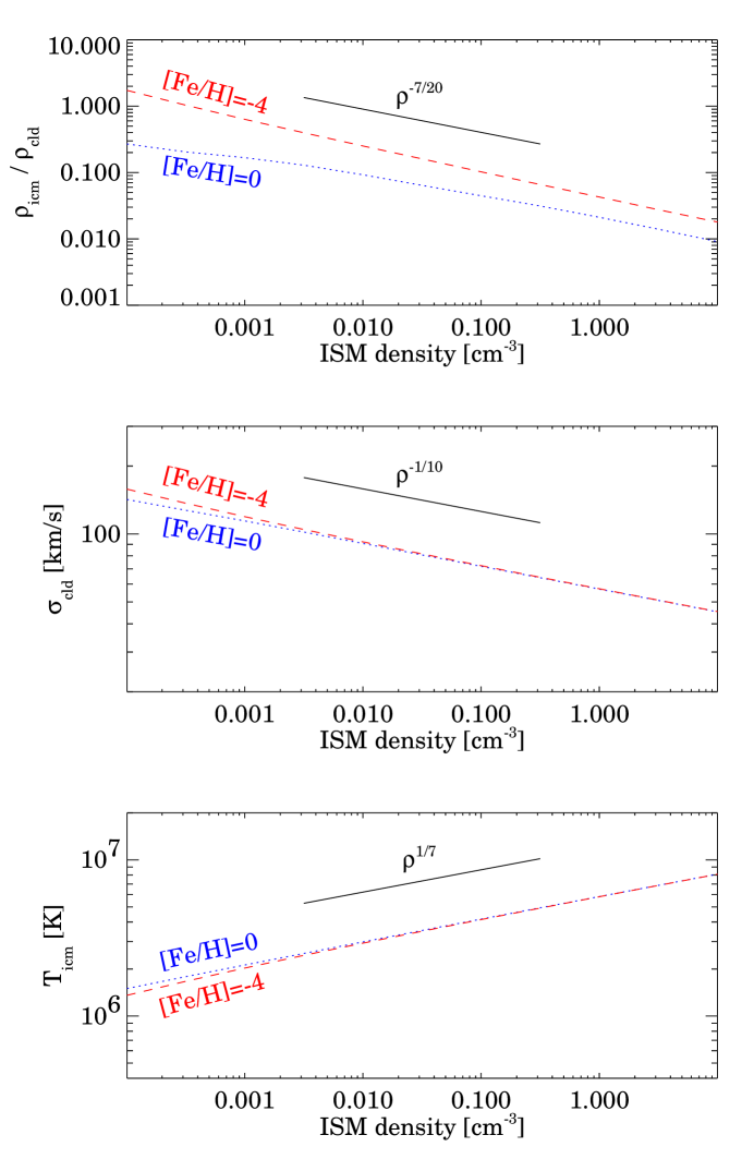
Figure 4: The three panels show the density dependence of the intercloud to cloud mass ratio, the cloud velocity dispersion $\sigma_{\mathrm{cld}}$, and the hot gas temperature $T_{\mathrm{icm}}$ in a closed-box model where dynamical effects are neglected. The dotted and dashed lines show the [Fe/H] = 0 (solar metallicity) and the [Fe/H] = -4 cases and the full lines show the slopes given by the analytical approximations of eqns. 17–19.

For the analytical approach, we assume that, most of the ISM mass is in the cloudy medium and that the cloudy medium is in pressure equilibrium with the surrounding gas. Balancing the heating by SNe with the dissipation by cloud-cloud collisions and the cooling by radiation, and assuming that evaporation rates are equal to condensation rates, we get the following three relations:

$$\sigma_{\mathrm{cld}}\propto\left({\eta_{\mathrm{sf}}\eta_{\mathrm{cld}}\over\eta_{\mathrm{coll}}}\right)^{4/5}\cdot\rho^{-1/10}$$ (17)

$$T_{\mathrm{icm}}\propto\left({\eta_{\mathrm{sf}}\eta_{\mathrm{cld}}\over\eta_{\mathrm{coll}}}\right)^{2/7}\cdot\left({\eta_{\mathrm{sf}}\eta_{\mathrm{cond}}\over\eta_{\mathrm{evap}}}\right)^{2/7}\cdot\rho^{1/7}$$ (18)

$${\rho_{\mathrm{icm}}\over\rho_{\mathrm{cld}}}\propto\left({\eta_{\mathrm{sf}}\eta_{\mathrm{cld}}\over\eta_{\mathrm{coll}}}\right)^{3/10}\cdot\left({\eta_{\mathrm{sf}}\over\eta_{\mathrm{cool}}}\right)^{1/2}\cdot\rho^{-7/20}$$ (19)

Here $\rho$ is the average density of the ISM (clouds and hot gas). These equations confirm that there is only a weak dependence of $\sigma_{\mathrm{cld}}$ and $T_{\mathrm{icm}}$ on the average ISM density. They are shown in Fig. 4 for comparison with the numerical results.

In the previous discussion, we neglected metallicity effects. However, metallicity can be important because it increases the cooling efficiency. The dashed lines in Fig. 4 show the numerical equilibrium relations for an extremely metal-poor gas ([Fe/H] = -4). The effects of low gas metallicities are similar to a low cooling efficiency $\eta_{\mathrm{cool}}$. In both cases, the gas temperature $T_{\mathrm{icm}}$ stays nearly constant, because the lower cooling efficiency is balanced by a higher gas density $\rho_{\mathrm{icm}}$. The self-regulating character of the interaction network again is obvious. The equilibrium system is in a balance of forward and reverse reaction rates. Any stress that alters one of these rates makes the system shift, so that the two rates eventually equalize (Le Chatelier’s principle).

In spite of the self-regulating character of the interaction network it is necessary to solve the full interaction network during a simulation, because processes on different timescales are involved that compete with the dynamical evolution. For example, heating processes or cloud dissipation may take longer than dynamical changes. Equilibrium solutions of the interaction network can be used only to study the general behaviour of a star-gas system where dynamical processes are slow, but would not be able to describe, e.g., the outflow of hot gas.

3.4.10 Sensitivity to free parameters

Most of the parameters in this multi-phase ISM description ($\eta$’s) can be constrained either from theory or from observations. The two most important parameters in the model are the star formation efficiency $\eta_{\mathrm{sf}}$, and $\eta_{\mathrm{coll}}$ which controls the dissipation rate. These parameters are of special interest because they both influence the velocity dispersion of the cloudy medium and thus the settling of the baryonic matter.

In Table 1 we list the parameters of the interaction network together with their upper and lower limit values. These are discussed in the subsections above. For $\eta_{\mathrm{evap}}$ and $\eta_{\mathrm{coll}}$, where there is little constraint, we have used a large range to illustrate that even in this case the resulting changes to the equilibrium are not large. It is obvious from the analytical model above that $\eta_{\mathrm{sf}}$ ($\eta_{\mathrm{cld}}$, $\eta_{\mathrm{coll}}$) have influence on $\sigma_{\mathrm{cld}}$, $T_{\mathrm{icm}}$ and $\rho_{\mathrm{icm}}$, while $\eta_{\mathrm{evap}}$ ($\eta_{\mathrm{cond}}$) can change only $T_{\mathrm{icm}}$, and by varying $\eta_{\mathrm{cool}}$ one can shift the gas-to-cloud mass ratio. Using the extreme values for the parameters given in Table 1 we obtain the uncertainties of $\sigma_{\mathrm{cld}}$, $T_{\mathrm{icm}}$, and $\rho_{\mathrm{icm}}$ (column 5, 6, and 7 of Table 1). This shows that even large changes of the parameter values lead only to moderate variations in $\sigma_{\mathrm{cld}}$, $T_{\mathrm{icm}}$, and $\rho_{\mathrm{icm}}$. From these numbers we conclude that $\sigma_{\mathrm{cld}}$, $T_{\mathrm{icm}}$, and $\rho_{\mathrm{icm}}$/$\rho_{\mathrm{cld}}$ are accurate to a factor of 2 in our model.

parameter	eqn.	range	std. value	$\sigma_{\mathrm{cld}}$ / $\sigma_{\mathrm{cld}}^{\rm std}$	$T_{\mathrm{icm}}$ / $T_{\mathrm{icm}}^{\rm std}$	$\rho_{\mathrm{icm}}$ / $\rho_{\mathrm{icm}}^{\rm std}$
$\eta_{\mathrm{sf}}$	8	$(5-30)\times 10^{-4}$	$5.3\times 10^{-4}$	1.0-4.0	1.0-2.7	1.0-4.0
$\eta_{\mathrm{cld}}$	10	0.02 - 0.1	0.05	0.5-1.7	0.8-1.2	0.8-1.2
$\eta_{\mathrm{cool}}$	11	2.3-10	5	1.0	1.0	1.5-0.7
$\eta_{\mathrm{coll}}$	13	0.013-0.5	0.025	1.7-0.1	1.2-0.4	1.2-0.4
$\eta_{\mathrm{evap}}$	15	$(0.1-10)\times 10^{-19}$	$10^{-19}$	1.0	1.9-0.5	1.0
$\eta_{\mathrm{cond}}$	16	0.3-1.0	0.5	1.0	0.9-1.2	1.0

Table 1: Parameters of the model interaction network and the equations in which they are defined. Column 3 shows lower and upper limits for the parameters, column 4 the standard values used in the simulations, and columns 5, 6, and 7 give the equilibrium $\sigma_{\mathrm{cld}}$, $T_{\mathrm{icm}}$, and $\rho_{\mathrm{icm}}$ resulting with the maximum and minimum parameter values, normalized by those obtained for the standard model values.

3.5 Gravitation

Gravitation is a long range force that couples the baryonic and the dark matter and it is the main driver of the galactic evolution. To determine the gravitational potential, we first map all stars, the different phases of the ISM and the dark matter onto one grid. Then, depending on the kind of grid (equidistant or logarithmically spaced) we solve the Poisson equation with a FFT (fast Fourier transformation) or a SOR (successive over-relaxation with Chebeyshev acceleration) method. The gravitational forces are calculated from the potential at every point.

3.6 Initial conditions and code set-up

The present simulations used a logarithmic $81^{3}$ grid with a spatial resolution of $370\mathrm{\,pc}$ in the inner parts and $5\mathrm{\,kpc}$ in the outer halo. The timestep lengths, which in most cases are limited by the interaction processes, are of the order of $10^{4}-10^{5}\mathrm{\,yr}$. The simulations start at a redshift $z=4.85$ corresponding to $t=1.2\mathrm{\,Gyr}$ in a $\Lambda$CDM cosmology. Initially the dark halo has a mass of $2.1\times 10^{10}\mathrm{\,M}_{\sun}$, distributed over a $30\mathrm{\,kpc}$ sphere. During the evolution, the halo grows by accretion to a size of $500\mathrm{\,kpc}$ with an enclosed mass of $1.8\times 10^{12}\mathrm{\,M}_{\sun}$. The baryonic-to-dark matter ratio of the accreted mass is fixed at 1:5, which finally amounts to $3\times 10^{11}\mathrm{\,M}_{\sun}$ of baryonic matter inside the $r_{200}$ radius. The accretion rate, taken from cosmological simulations (Kauffmann et al., 1999, see Section 3 and Fig.5) decreases from $32\mathrm{\,M_{\odot}\,yr^{-1}}$ at $z=4.85$ ($1.2\mathrm{\,Gyr}$) to $8.1\mathrm{\,M_{\odot}\,yr^{-1}}$ at $z=0$ ($13.5\mathrm{\,Gyr}$). The baryonic matter outside the $r_{200}$ radius consists of ionized ($T>10^{4}K$) primordial gas at the virial temperature. The cooling time of this gas is short compared to the collapse time. On this time-scale clouds form which can then dissipate kinetic energy and collapse inside the dark halo. Thereafter the collapse is only delayed by stellar feedback processes. We have confirmed that starting with a cloudy gas medium leads to a very similar evolution. Initially, the accreted baryonic matter, like the dark matter, is in spherical rotation (eqn.1) with a spin parameter $\lambda=0.05$. It grows from inside-out and the mass with the highest specific angular momentum is accreted at late times.

Figure 5: Baryonic mass infall rate (MIR, full line) into inner $20\mathrm{\,kpc}$ and across the $r_{200}$ radius (dashed line).

4 The formation history

The present simulation describes the formation and subsequent evolution of a disk galaxy in a slowly growing dark halo. The halo grows by accreting dark and baryonic matter in spherical shells with an accretion rate that is derived from cosmological simulations in a $\Lambda$CDM universe (Kauffmann et al., 1999, see Section 3.1), with a baryonic mass fraction of 1/6. The dark and baryonic matter have initial $\lambda=0.05$ and specific angular momentum distribution similar to that from Bullock et al. (2001). Star formation, feedback, and gas physics of the baryonic component are described within a two-phase ISM model (see Section 3.3). The dynamics of the gas and stars is treated separately. The simulations start at $z=4.85$ ($t=1.2\mathrm{\,Gyr}$) with a mixture of dark matter and gas, but no stars. At redshift $z=4.85$ the dark halo mass exceeds $2.0\times 10^{10}\mathrm{\,M}_{\sun}$, which is twice the mass resolution of the cosmological simulations on which our halo model is based.

4.1 Collapse and star formation history

The accreted primordial gas quickly reaches an equilibrium between the cold and hot phases with most of the mass in the cold clouds. It can then dissipate its kinetic energy and begins to collapse inside the dark halo. The strong collapse takes place in a redshift interval between $z=1.8$ ($3.6\mathrm{\,Gyr}$) and $z=0.8$ ($6.6\mathrm{\,Gyr}$). With a duration of $\sim 3\mathrm{\,Gyr}$, its period exceeds the free-fall time at the $r_{200}$ radius by a factor of 3.4. This late and delayed collapse, which is in contradiction to simple collapse scenarios, is caused by stellar feedback in conjunction with the initially shallow gravitational potential of the halo.

The baryonic mass infall rate (MIR) across the $r_{200}$ radius and into the inner $20\mathrm{\,kpc}$ is shown in Figure 5. At early times the gas fallen through $r_{200}$ has not yet reached the inner $20\mathrm{\,kpc}$ because of the delay from feedback. With the growing mass of baryons the dissipation increases and the infall into the centre accelerates, until the combination of feedback from the growing star formation rate and decreasing infall rate through $r_{200}$ reverses this trend and the MIR into $20\mathrm{\,kpc}$ begins to decrease again at $z\simeq 1.2$. At late times ($z\mathrel{\hbox to0.0pt{\lower 3.0pt\hbox{$\mathchar 536\relax$}\hss}\raise 2.0pt\hbox{$\mathchar 316\relax$}}0.3$) a significant fraction of the infalling gas has too much angular momentum to arrive in the central $20\mathrm{\,kpc}$, so that the rate of infall into $20\mathrm{\,kpc}$ becomes lower than that through $r_{200}$. The mass of the galaxy increases rapidly and at $z=1.2$ ($5\mathrm{\,Gyr}$) already $10^{11}\mathrm{\,M}_{\sun}$ of baryonic matter has been accreted. At $z=0$, 2/3 of the total baryonic mass of $3\times 10^{11}\mathrm{\,M}_{\sun}$ has collapsed into the inner $20\mathrm{\,kpc}$ of the dark matter halo and has formed the luminous galaxy, leading to a dark-to-baryonic matter ratio of 3%, 10% and 30% inside galactocentric radii of 1, 3, and $10\mathrm{\,kpc}$, respectively.

The star formation rate integrated over the central $20\mathrm{\,kpc}$ is shown in Figure 6. This increases steeply to a maximum of $\approx 50\mathrm{\,M_{\odot}\,yr^{-1}}$ at $z=1$ ($5.75\mathrm{\,Gyr}$). At that time, the gas consumption by the star formation process is balanced to 80% by infall and to 20% by the stellar mass return. Afterwards the infall rate decreases to $5\mathrm{\,M_{\odot}\,yr^{-1}}$, at $z=0$, while the stellar mass return stays nearly constant at a rate of $10\mathrm{\,M_{\odot}\,yr^{-1}}$. This explains the different shapes of the curves in Figs. 5, 6 at late times.

Figure 6: Star formation rate (SFR) in the inner $20\mathrm{\,kpc}$ of the dark halo. The star formation rate peaks slightly later than the MIR (Fig. 5).

4.2 Sequential formation of halo, bulge and disk

Figures 7, 8 show the spatial distributions of the gas and stars as a function of redshift. In general terms, star formation out of the dissipating cloud medium proceeds from halo to disk and from inside out. Thus the earliest stars at redshifts $z>2$ form in the whole volume limited by the $r_{200}$ radius (halo formation), with a concentration to the central bulge region. At a redshift of $z=1.3$ ($4.7\mathrm{\,Gyr}$), a (thick) disk component first appears. Later the star formation is concentrated to the equatorial plane, and at late times most of the star formation occurs in the outer disk.

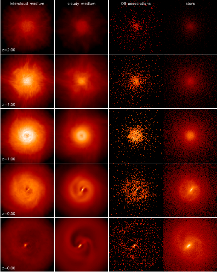
Figure 7: Face-on surface density of the ionized gas, the cloudy medium, the OB-associations and the stars at different redshifts. Each column shows the evolution of one component between redshift $z=2$ and $z=0$. Each panel has a size of $50\times 50\mathrm{\,kpc}$.

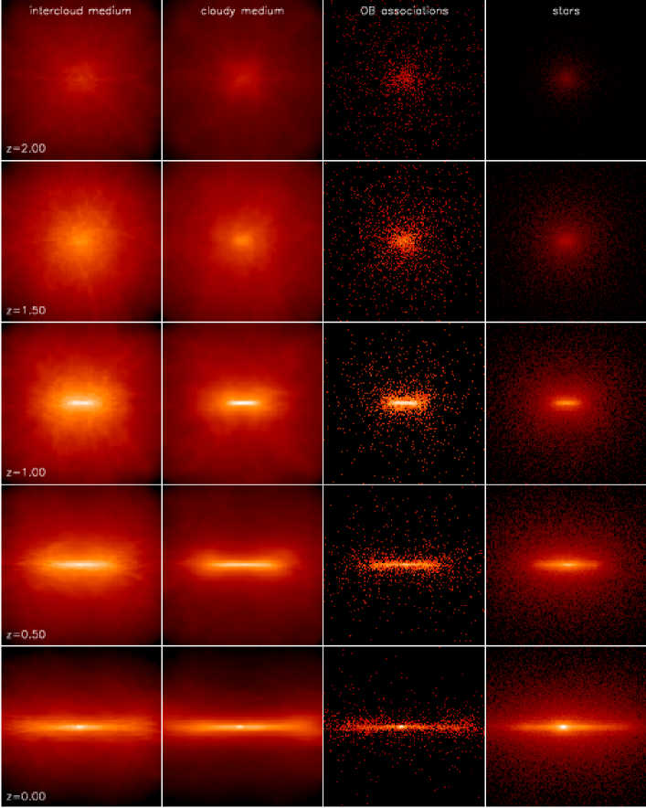
Figure 8: Same as Fig. 7, but for the edge-on view.  

Around $z=1.2$ the infall of gas can no longer compensate the gas consumption by star formation in the inner disk. This is because the infalling molecular cloud medium now has higher specific angular momentum, so that its infall timescale becomes longer than the central star formation timescale. As a result, the region of highest star formation density moves radially outwards from the centre and a ring (Fig. 7, $z=1$ panels) forms. This ring grows to a radius of $\sim 4\mathrm{\,kpc}$ before, at redshift $z=0.85$ ($6.4\mathrm{\,Gyr}$), the disk becomes unstable. Within $150\mathrm{\,Myr}$ the ring then fragments, and for a short time ($\approx 150\mathrm{\,Myr}$) a very elongated bar is formed with exponential major-axis scale-length of $5.9\mathrm{\,kpc}$ and axis ratio of 12:2:1. Fig. 9 shows that after this transient period the bar length decreases, and a bar-bulge with axial ratios $\sim$3:1.4:1 develops which includes the old bulge component formed in the early collapse.

Already during this bar formation process the galaxy starts to build up the outer disk. This disk is the youngest component in the model galaxy, even though the oldest disk stars are as old as the halo stars. The disk grows from inside-out, because the early accreted mass has low specific angular momentum (see the last columns of Fig. 7 and Fig. 8). In parallel, the vertical scale-height in a fixed radial range decreases; this is shown in Fig. 10 for the range $3-10\mathrm{\,kpc}$. The more pronounced settling of the cloudy medium to the equatorial plane at late times is due to (i) more efficient cooling because of higher metallicity, (ii) higher gas density and, thus, dissipation rate for gas near the angular momentum barrier in a deeper potential well. The final disk thickness in Fig. 10 of $\approx 500\mathrm{\,pc}$ is set by the resolution the present model.

After the bar-bulge has formed, two trailing spiral arms appear in the disk which are connected to the bar-bulge. At the beginning the two spiral arms are symmetric and of the same size. However, in the further evolution a persistent lopsidedness of the galaxy develops. The resulting off-centre motion of the bulge-bar brings one arm nearer to the bulge-bar, and the more distant spiral arm becomes more prominent over a wider winding angle (Fig. 7). The lopsidedness may be produced by the dark halo which is here described as an external spherically symmetric potential component, even though in the inner galaxy the baryonic matter dominates the gravitational potential. The effect that such perturbations can produce lopsided galaxies is well known (Levine & Sparke, 1998; Swaters et al., 1999).

We expect this evolutionary sequence to be more or less typical of any dissipative collapse in a growing dark matter halo, unless it is interrupted by substantial mergers. The following modelling uncertainties may further modify the evolution as described above. (i) The assumed dissipation parameter is uncertain. If in reality dissipation is significantly more efficient than in the model, and in addition stars form only above a certain density threshold (Kennicutt, 1998), the gas would fall into the disk much more rapidly without significant star formation. In this case formation of stars in the halo and thick disk may be substantially suppressed. Also, in this case the velocity dispersion of the cloudy medium in the disk would decrease. Then the gaseous disk may fragment in local instabilities before a global disk instability sets in, so that more material would dissipate to the centre and contribute to the bulge. (ii) The precise angular momentum distribution (as compared to the universal average distribution assumed) will influence the detailed inside-out formation of the disk. For example, the formation of a ring in the present model would likely be suppressed by increasing the amount of low angular momentum gas falling in at redshift $z\simeq 1$. (iii) When small-scale initial fluctuations lead to the formation of sub-galactic fragments that merge before the main collapse, the mass of the bulge component would be substantially greater, and its dynamical structure determined by the merging process (Steinmetz & Navarro, 2002).

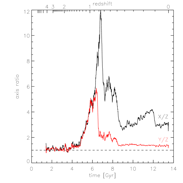
Figure 9: Evolution of the bar-bulge axis ratios. z indicates the vertical direction and x and y the major and minor axes of the bar. The bar forms from a disk instability at time $6.4\mathrm{\,Gyr}$ and settles to a triaxial bulge with axis ratios $\sim$3:1.4:1 at late times.

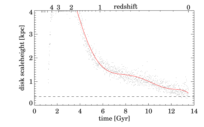
Figure 10: Evolution of the vertical scale height of the stellar disk between radial distances $3-10\mathrm{\,kpc}$. This part of the disk forms later than the average of all stars shown in Fig. 5. The scale heights in small rings are shown as dots and the radial average is drawn as a full line. The dashed line indicates the spatial resolution limit of $370\mathrm{\,pc}$.

4.3 Global chemical evolution

The chemical evolution of the model proceeds in three steps. First, there is the collapse phase, lasting until $z\simeq 0.6$. Then two quasi-equilibrium phases follow in which first ($z=0.6-0.3$) the mass infall and later ($z=0.3-0.0$) the stellar mass return determines the star formation rate (see Figs. 5, 6). These three phases are clearly visible in the chemical enrichment history of the cloudy medium. This is shown in Fig. 11, where we have plotted the Zn/H metallicity normalized to the solar value because Zn is believed to not be depleted onto dust grains. The Zn/H abundance was reconstructed from the fiducial SN I and SN II elements as described in Section 3.

Figure 11: Average $\@element{\mathrm{Zn}}$/$\@element{\mathrm{H}}$ abundance (linear scale) of the ISM and the stars in the inner $20\mathrm{\,kpc}$ of the model galaxy.

The initial collapse of the baryonic material produces a first generation of stars which already at $z=2$ has synthesized enough metals to increase the average metallicity to $\approx-1$. During the late collapse phase the star formation rate exceeds the MIR and the metallicity increases fast. Then in the second phase, the star formation rate is proportional to the MIR and the metallicity increases only slowly. In the final phase, the star formation rate is again higher than the MIR and the metallicity increases more rapidly (Fig. 11).

The chemical enrichment histories of the hot gas, cloudy medium, and stars (shown separately in Fig. 11) are very different from the predictions of multi-phase closed box models. In these models the hot ionized gas always has the highest metallicity, followed by the molecular cloud medium and the stars. This is different in our model, because stars, clouds and gas have different spatial distributions. Most of the ionized hot gas is located in the halo, while the molecular clouds and stars are preferentially found in the disk and bulge, where the gas densities and metallicities are high. After a brief initial period the average metallicity of the stars exceeds that of the cloudy medium, because the stars form from gas that is more concentrated to the equatorial plane and thus more metal-rich than the average cold gas medium.

An interesting feature in Fig. 11 is the constant [Zn/H] $\approx 0.4$ of the hot gas from redshift $z=1$ until the present epoch. A large fraction of this gas occupies the galactic halo, where the star formation rate is low. Two processes keep the halo metallicity at a constant level: Gas flows from the bulge and the disk transport heavy elements into the halo. There it mixes with the existing ISM and with infalling low metallicity gas. In this way the metallicity in the halo gas can remain constant over a long time.

A similar enrichment can be observed in the disk. During the collapse the star formation and the metal production is concentrated to the inner galaxy. From there, the metal-rich gas expands into the disk. This disk pre-enrichment causes a lack of metal-poor stars (“G-dwarf problem”, see Section 5), similar to that observed in the Milky Way.

We find a global age-metallicity relation and also a [O/Fe] to [Fe/H] relation, which are consistent with Milky Way observations. These relations are much more influenced by the choice of stellar yields, resp. the star formation history, than by the details of the galactic model, and have been found in previous galactic models as well (e.g. Steinmetz & Müller, 1994; Timmes et al., 1995; Samland, 1998). However, the pre-enrichment of the galactic disk, explaining the so-called “G-dwarf problem” and the sub-solar abundances in the outer halo gas are a result of dynamical processes and are therefore strongly influenced by the galactic model. The same is true for relations connecting the kinematics and chemical composition of stars; see Section 5.7.

In Fig. 12 we compare our results with the [Zn/H] data for damped Ly$\alpha$ systems (Pettini et al., 1999; Prochaska et al., 2001), using [Zn/H] because [Fe/H] may be depleted by dust. Damped Ly$\alpha$ systems are an important test for galactic models. If they are associated with forming disk galaxies, they can be used to measure the metallicity of the ISM of young, gas rich galaxies at high redshifts. The Ly$\alpha$ systems on average show only a mild evolution in [Zn/H] for $z\approx 2-3$. Even though we consider only a single model with its specific evolutionary history, the predicted metallicity range as a function of redshift is consistent with the data. From the model we thus infer that the time needed to increase the disk metallicity to the typical values observed in Ly$\alpha$ systems is $\sim 1\mathrm{\,Gyr}$. The shaded area in Fig. 12 shows the range of metallicities from different locations in the model at redshifts $z>1.6$. Fig. 12 also shows the early [Zn/H] evolution of the hot ionized gas (dashed line). This should be representative for the average metallicity of metal-enriched clouds forming in the low density halo ISM, and thus for absorption of background quasars along halo lines-of-sight.

4.4 The ISM at $z=0$

At $z=0$, $5.6\times 10^{10}\mathrm{\,M}_{\sun}$ (15.7%) of the initial baryonic mass of $3\times 10^{11}\mathrm{\,M}_{\sun}$ is still in the form of gas. The distribution of this late ISM is spatially more extended than that of the stars and the mass ratio of ISM to stars increases with distance from the galactic centre. Inside $10\mathrm{\,kpc}$, only about 2% of the baryonic mass is still in the ISM, but inside $60\mathrm{\,kpc}$ the fraction is already 43%. 75% of the ISM mass is in the cold and warm phases (molecular and atomic gas), but a significant fraction of 25% is hot and ionized. This hot gas extends far out into the halo and fills most of the halo volume (see Fig. 8). As discussed in the previous subsection, the hot gas is the chemically least enriched component at late times.

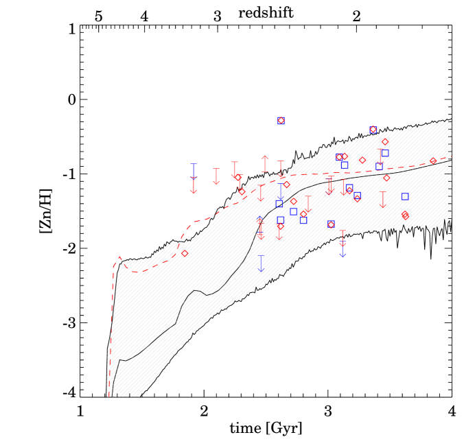
Figure 12: Redshift evolution of the average zinc abundance [Zn/H] of the cloudy medium (full line) inside a galactocentric radius of $20\mathrm{\,kpc}$. The shaded area shows the range of [Zn/H] metallicities in the model over this region. The points are data for damped Ly$\alpha$ systems from Pettini et al. (1999) and Prochaska et al. (2001), plotted as squares and rhombi, respectively. The general trend of the model curve is consistent with the observed damped Ly$\alpha$ abundances. The dashed line indicates the metallicity evolution of the hot gas component, which fills most of the galactic halo.

5 Formation of galactic components

The model presented in this paper describes the formation of a massive disk galaxy with a total luminous mass of $2\times 10^{11}\mathrm{\,M}_{\sun}$ inside $20\mathrm{\,kpc}$ and a disk rotation velocity of $270\mathrm{\,km\,s^{-1}}$ at a radius $10\mathrm{\,kpc}$, about 2.5 times more massive than the Milky Way. The galaxy model forms from inside-out radially and from halo to disk vertically. In Fig. 6 one can clearly see halo, bulge, and disk components, which as described in Section 4 form sequentially in this order. The model contains the full spatially resolved dynamical and chemical information for all of these components. With this information it is possible to study the detailed consequences for the stellar kinematics and abundances, that are implied by the assumptions made for the galaxy formation scenario and the modelling of the various physical processes involved, and to compare to a variety of observational data.

Figure 13 shows average properties of the model stars at redshift $z=0$: age, metallicity, [O/Fe], and rotational velocity. These vary continuously as a function of position in the meridional plane ($R,Z$), in a way that reflects the interplay between star formation and enrichment on the one hand, and the vertically top-down and radially inside-out dynamical formation on the other hand. Thus, the oldest stars can be found at low radial distances in the halo and the youngest stellar populations are located in the outer galactic disk. Because mean age and mean metallicity vary as a function of position, global mean values for age or metallicity are not sufficient to characterize the stellar population of a galaxy. Notice also that stars at a given mean age or metallicity can be found in a variety of positions.

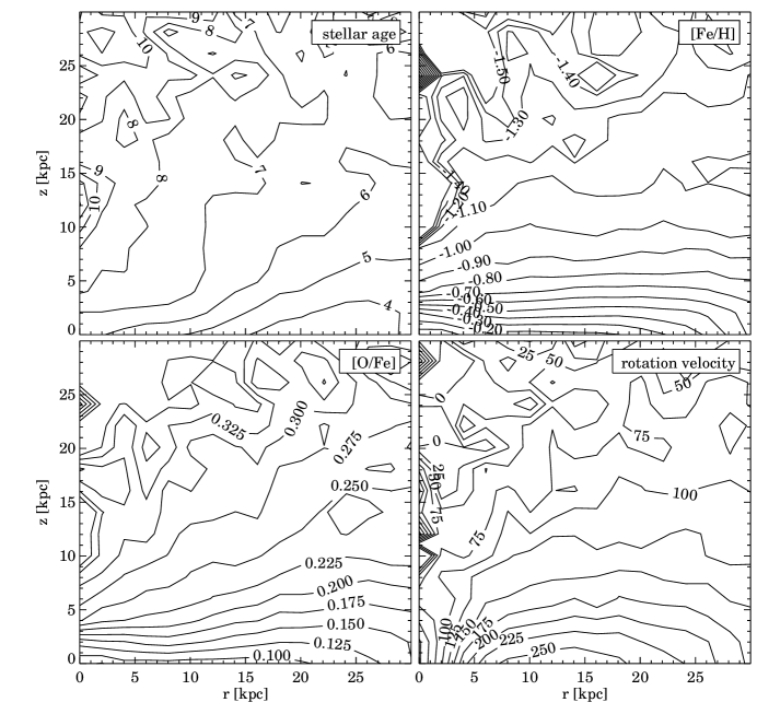
Figure 13: The panels show the mean stellar age, [Fe/H], [O/Fe], and mean rotation velocity $V$ of the model stars at redshift $z=0$, in the meridional plane as a function of radial ($R$) and vertical distance ($Z$) from the galaxy’s centre. The mean stellar ages are given in Gyr, and the units of the velocities are $\mathrm{\,pc\,Myr^{-1}}=0.98\mathrm{\,km\,s^{-1}}$.

In Fig. 14 we plot the complete distribution of model stars at redshift $z=0$ in the plane of rotational velocity $\mathrm{\,v_{rot}}$ versus metallicity [Fe/H]. This shows the expected evolution from non-rotating, low-metallicity stars formed early in the collapse to a rotating disk-like, metal-rich population formed at late times. However, this evolution is by no means described by a single dependence of $\mathrm{\,v_{rot}}$ on [Fe/H]; rather there is large scatter in $\mathrm{\,v_{rot}}$ at given metallicity, especially at low [Fe/H] values. In addition, there are also at least two concentrations of stars visible, at [Fe/H] $\simeq-0.4$ and [Fe/H] $\simeq 0.1$.

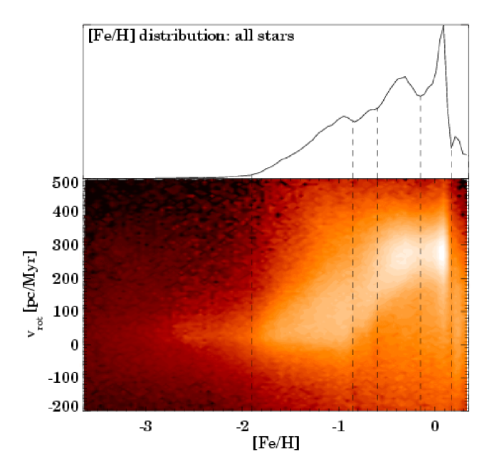
Figure 14: Lower panel: Distribution of model stars in the metallicity–rotation velocity plane. Rotation velocities are perpendicular to the total angular momentum vector and are in $\mathrm{\,pc\,Myr^{-1}}$. Upper panel: total metallicity distribution of all model stars, projecting along the rotation velocity axis. The dashed lines separate the subpopulations discussed in the text.

The top panel of Fig. 14 shows a [Fe/H] histogram of all stars, projecting along the $\mathrm{\,v_{rot}}$ axis. Based on this histogram, we will now study the stellar populations in the different parts of Fig. 14 separated by the dashed lines. In first order these might be described as extreme halo, inner halo, metal-weak thick disk, thick disk, thin disk, and central bulge components, somewhat reminiscent of the similar components known in the Milky Way. However, we do not intend to imply a detailed correspondence with the Milky Way components; there are significant differences with the present model. Recall that the dark and baryonic masses of this model are larger than in the Milky Way, and especially the dissipation parameter of the model may not be typical for the Milky Way. Nonetheless, studying these components is useful to understand the course of the dynamical evolution and chemical enrichment in dissipative, star-forming collapse, and we will for definiteness use the Milky Way terminology in the following discussion of the properties of these populations.

5.1 [Fe/H]$<-1.9$ (“Extreme halo”)

This component comprises all stars with [Fe/H] $<-1.9$; these stars form before the collapse and simultaneous spin-up of the gas goes under way. As the left row of Figure 15 shows, these stars form mostly in the first two Gyr after the start of the simulation (at time $1.2\mathrm{\,Gyr}$), but there is a small ongoing star formation in the halo even to late times from infalling low-metallicity gas (remember that we have not imposed a density threshold for star formation in this model). These stars have [O/Fe] near 0.4 typical for enrichment by SNe II. Their spatial distribution is nearly spherical, they rotate slowly if at all, and they have an asymmetric, broad distribution of eccentricities biased towards radial orbits. Here we have defined eccentricity as $e=(r_{\rm max}-r_{\rm min})/(r_{\rm max}+r_{\rm min})$ where $r_{\rm max}$ and $r_{\rm min}$ are the maximum and minimal three-dimensional radii of the orbit. The relative lack of low-eccentricity orbits at these metallicities (see Section 5.7) may be due to our neglect of small-scale structure in the initial conditions; compare with Bekki & Chiba (2001).

5.2 $-1.9<$[Fe/H]$<-0.85$ (“Inner halo”)

Stars in this component have a metallicity range $-1.9<$ [Fe/H] $<-0.85$, covering the spin-up phase until the first minimum in the [Fe/H] histogram in Fig. 14. These stars form a more flattened spheroidal distribution with a flat density profile. They rotate with $\sim 70\mathrm{\,km\,s^{-1}}$, and the eccentricity distribution is less radially biased than for the extreme halo component. This component forms partly during the phase of rapid increase in the global star formation rate (Fig. 6), but there is also a younger part forming until late times. Here the selection in metallicity is important: the older part of these stars forms at relatively small radii when the metallicity there reaches the selected range, while the younger component forms at progressively larger radii from infalling low-density gas mixed with outflowing enriched material. This younger component may not form in real galaxies if stars can only form above a density threshold, as inferred from observations by Kennicutt (1998). Further simulations also showed that a larger dissipation parameter (see Section 3.4.6) leads to a faster settling of the clouds into the disk and this suppresses the star formation in the halo at late times.

5.3 $-0.85<$[Fe/H]$<-0.6$ (“Metal-weak thick disk”)

These stars with $-0.85<$[Fe/H]$<-0.6$ are intermediate in their rotational properties between a halo and a disk population (see Fig. 14). As Fig. 15 shows their spatial distribution is already strongly flattened. They have a sizeable rotation with peak of the distribution at $\mathrm{\,v_{rot}}\simeq 150\mathrm{\,km\,s^{-1}}$, around 50-60% of the circular velocity. The eccentricity distribution is broad and centred around 0.5. The oldest stars of this component form at around the peak of the global star formation rate when the gas still has [O/Fe] $\simeq 0.3$. A slightly larger fraction of stars in this range of [Fe/H] forms continuously until late times, at progressively larger radii, again favoured by the lack of star formation threshold. These stars are already enriched by SN Ia, as visible in their [O/Fe] distribution.

5.4 $-0.6<$ [Fe/H] $<-0.15$ (“Thick disk”)

This component with $-0.6<$[Fe/H]$<-0.15$ is one of the distinct components in Fig. 14, and is clearly dominated by a disk component in its rotational properties and eccentricity distribution. However, Fig. 14 shows that it also contains intermediate metallicity retrograde stars, showing that this metallicity selection also includes part of the bulge. These bulge stars cause the peak in the age distribution at $\sim 5\mathrm{\,Gyr}$, with high [O/Fe]. The disk part has a relatively narrow distribution in [O/Fe] centred around $\sim 0.13$.

5.5 $-0.15<$[Fe/H]$<0.17$ (“Thin disk”)

The thin disk component, selected in the interval $-0.15<$ [Fe/H] $<0.17$, is characterized by near-circular orbits and a high rotation velocity, about $270\mathrm{\,km\,s^{-1}}$. This component forms with an approximately constant star formation rate and has mostly near-solar [O/Fe]. As in the previous thick disk component, a contribution from bulge stars is included by the metallicity selection. The thin disk shows the bar and spiral arms clearest; see the top panels in Fig. 15. In time, it forms from inside out due to the accretion of material with progressively larger angular momentum.

The thin disk shows only a shallow radial metallicity gradient of $0.02$ dex/kpc, which is due to efficient mixing of the disk ISM by the galactic bar. Beyond $16\mathrm{\,kpc}$, where the mixing is not very efficient, a steeper metallicity gradient of $0.07$ dex/kpc is established. See also Martinet & Friedli (1997) who found strong metallicity gradients only in non-barred galaxies. The metal production by the bulge and the mixing by the bar lead to a pronounced pre-enrichment of the disk, which is visible in Fig. 16 by the lack of metal-poor stars.

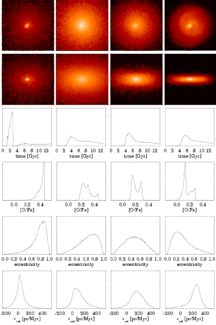
Figure 15: Properties of model subcomponent selected by metallicity according to the dashed lines in Fig. 14. Columns from left to right show all stars with [Fe/H] $<-1.9$ (“Extreme halo”), $-1.9<$ [Fe/H] $<-0.85$ (“Inner halo”), $-0.85<$ [Fe/H] $<-0.6$ (“Metal-weak thick disk”), $-0.6<$ [Fe/H] $<-0.15$ (“Thick disk”), $-0.15<$ [Fe/H] $<0.17$ (“Thin disk”), and [Fe/H] $>0.17$ (“Inner bulge”). For each of these components, the panels from top to bottom show the face-on projection onto the disk plane, edge-on projection, distribution of formation times, [O/Fe] distribution, eccentricity distribution, and distribution of rotation velocities. The top two panels in each row show an area of $40\mathrm{\,kpc}\times 40\mathrm{\,kpc}$. Star formation in the model starts at time $1.2\mathrm{\,Gyr}$.

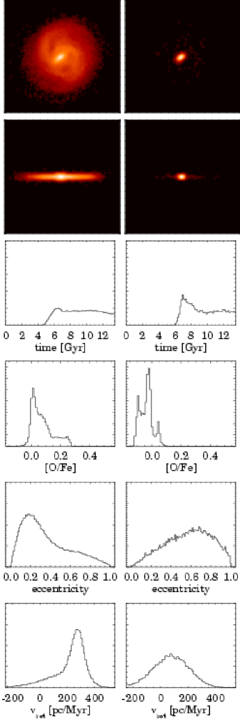
Figure 15: (continued)

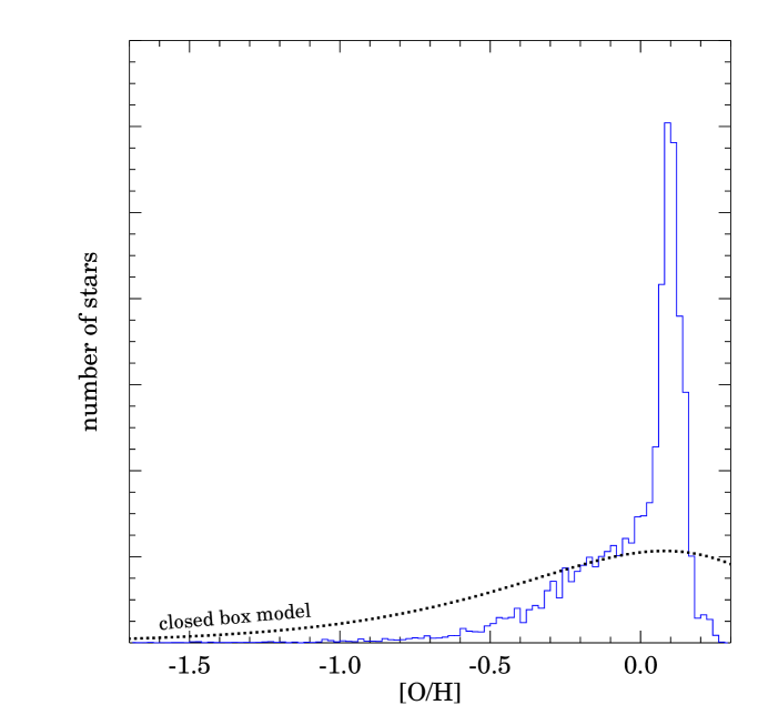
Figure 16: Distribution function of oxygen abundances of G-dwarfs, selected by mass, in the model galaxy at redshift $z=0$. All G-dwarfs in the equatorial plane with galactocentric distances between $9.5\mathrm{\,kpc}$ and $10.5\mathrm{\,kpc}$ are plotted. The dotted curve shows predictions of an instantaneous simple model with an effective yield $Y_{\rm eff}=Z_{\odot}$.

5.6 [Fe/H]$>0.17$ (“Inner bulge”)

The final metallicity component with [Fe/H] $>0.17$ consists mainly of stars in the central bulge. Notice that these most metal-rich stars do not form preferentially at late times; their age distribution is similar to that of the thick disk component. As the lower panels of Fig. 15 show, the metal rich inner bulge forms from $z\simeq 1$ in this model, rotates relatively slowly and has a broad eccentricity distribution.

The total bulge population includes this inner component and a second, more metal-poor component included in the metallicity range of the “thick disk”. Two subpopulations in the bulge is consistent with the observations of Prugniel et al. (2001), who find that galactic bulges in general consist of two different stellar components, an early collapse population and a population that formed later out of accreted disk mass.

5.7 Kinematics-abundance relations

The previous subsections have shown that while it is useful to select stellar components by metallicity, such a selection is not ideal because it lacks spatial and kinematical information. Vice-versa, a purely kinematical selection would mix stars from halo and bulge, or metal-poor and metal-rich disk. A more physical separation would involve spatial, kinematic, and abundance information. This is possible with models such as this, because the complete population of model stars is available, but will be deferred to a later paper. Here, we will only show two relations between kinematic and abundance parameters for all stars in the model, which further illustrate some of its properties.

Figure 17 shows the mean stellar rotation velocity as a function of metallicity [Fe/H] for all model stars. For [Fe/H] $<-2$ $\mathrm{\,v_{rot}}$ is independent of metallicity, at about $50\mathrm{\,km\,s^{-1}}$. It then rises roughly linearly with [Fe/H] until the disk rotation velocity is reached at [Fe/H] $\simeq 0.4$. As is apparent from Fig. 14, there is a large dispersion around the mean value except in the disk components. Figure 18 shows the mean orbital eccentricity and a sample of individual stellar eccentricities (defined in Section 5.1) as a function of metallicity. It is clear that at any metallicity, there is a large scatter in the orbital shapes. One of the causes of this is the very substantial deepening of the gravitational potential during the prolonged infall, which also affect orbits of stars formed early in the collapse. A second effect is that the turbulent velocities in the cloud medium are substantial during the collapse and during periods of large star formation rate, so that the stars made from these clouds inherit significant initial velocities. Thus all eccentricity distributions shown in Fig. 15 are fairly broad. When the various distributions shown in that figure are added with the appropriate mass weighting, a broad distribution results.

Figure 17: Mean stellar rotation velocity as a function of [Fe/H] for all model stars.

Both the dependence of $\mathrm{\,v_{rot}}$ on metallicity in Fig. 17 and that of eccentricity on [Fe/H] in Fig. 18 are similar to those observed in the Milky Way near the Sun (Chiba & Beers, 2000), even though our model was not made to match the Milky Way and does not in detail describe the Milky Way. The main conclusion we draw from diagrams like Figs. 17, 18 is that realistic dissipative collapses are much more complicated than the simple model put forward by Eggen et al. (1962) forty years ago. Therefore, inferring a merger history from the lack of rotation gradient with metallicity and a broad eccentricity distribution in the Milky Way halo is premature, irrespective of the fact that a fraction of the halo is likely to have been formed out of merging fragments (Ibata at al., 2001; Helmi et al., 1999; Chiba & Beers, 2000). The important question, about the relative importance of the disruption of small scale stellar fragments, merging of gaseous fragments, and star formation in smooth dissipative accretion, all within their dark matter halos, will need more detailed modelling and more data to answer. All of these processes are expected in current CDM galaxy formation theories. The present simulations show that feedback is important for the final properties of the stars formed.

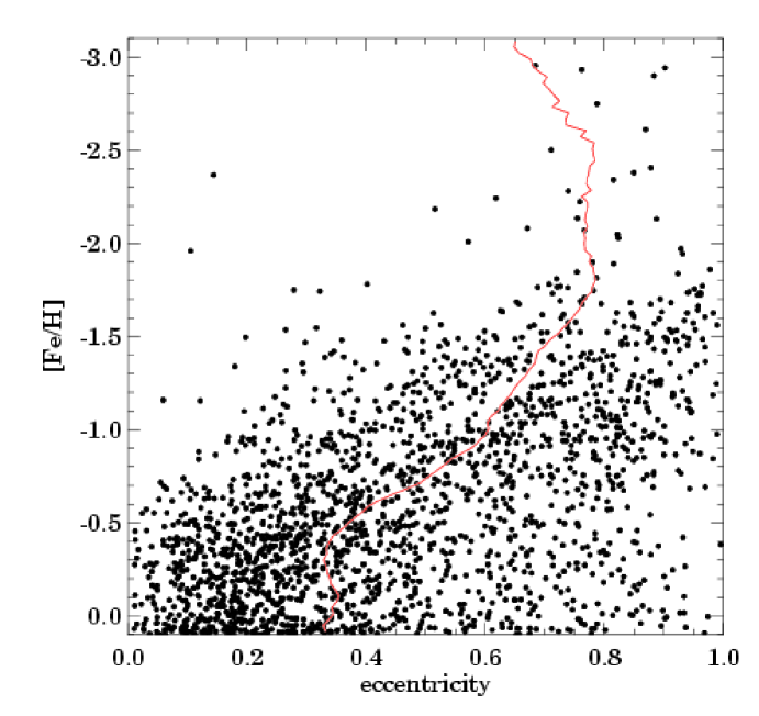
Figure 18: Sample of stellar orbital eccentricities and mean eccentricity of all stars in the model, as a function of metallicity.

6 Conclusions

We have presented a model for the dissipative formation of a large disk galaxy, inside a growing dark matter halo according to the currently favoured $\Lambda$CDM cosmology with $\Omega_{\Lambda}$=0.7, $\Omega_{0}$=0.3, $\rm h_{0}$=0.7. The dark halo mass accretion history is taken from the large-scale structure formation simulations of the GIF-VIRGO consortium (Kauffmann et al., 1999). We use a total dark matter mass of $1.5\times 10^{12}\mathrm{\,M}_{\sun}$, a total baryonic mass of $3\times 10^{11}\mathrm{\,M}_{\sun}$, a spin parameter $\lambda=0.05$, and an angular momentum profile similar to the universal profile found by Bullock et al. (2001).

We model the dynamics of stars and of two phases of the interstellar medium, including a phenomenological description of star formation, the most important interaction processes between stars and the ISM, and the feedback from massive stars and SNe. The dynamical evolution of the stars is treated with a particle-mesh code. For the dynamical description of the cold molecular and hot ionized gas components we use a three-dimensional hydrodynamical grid code. Linked to the N-body and hydrodynamical code is a Poisson solver for the self-gravity and an interaction network, including a description of star formation, the heating and enrichment of type Ia and II SNe, mass return by intermediate mass stars, the heating and cooling by radiation, dissipation in the cloudy medium, formation and evaporation of cold clouds in the hot intercloud medium. We discuss the range of uncertainty in the parameters that enter this description. Because of the self-regulation of these processes that is quickly established, even large changes in these parameters only lead to moderate changes, about a factor of 2, in the cloud velocity dispersion, hot gas temperature and ratio of hot to cold gas density.

The simulation starts at a redshift of $z=4.85$ with a dark halo of $2.1\times 10^{10}\mathrm{\,M}_{\sun}$. Inside the growing dark halo a disk galaxy forms, whose star formation rate reaches a maximum of $50\mathrm{\,M_{\odot}\,yr^{-1}}$ at redshift $z\approx 1$. Our main results can be summarized as follows:

1. The formation and evolution of a galaxy in a dissipative collapse scenario is much more complex than predicted by simple models. The energy release by SNe and massive stars (feedback) prevents the protogalaxy from a rapid collapse and delays the peak in the star formation to a redshift of $z\approx 1$. The prolonged formation time causes fundamental changes in the galactic shape, the kinematics of the stars, and the distribution of the heavy elements.

2. The galaxy forms radially from inside-out and vertically from halo-to-disk. The dynamics of the collapse strongly influences the star formation and chemical enrichment history, by modifying the gas density, cooling time, and thus star formation rate. The on average youngest and oldest stellar populations are found in the outer disk and in the halo near the galactic rotation axis, respectively. As a function of metallicity, we have described a sequence of populations, reminiscent of the extreme halo, inner halo, metal-poor thick disk, thick disk, thin disk and inner bulge in the Milky Way. The first galactic component that forms is the halo, followed by the bulge and the disk-halo transition region, and as the last component the disk forms.

3. An interesting feature of this model is the formation of a gaseous ring at a redshift of $z\simeq 1$ which collapses and forms a galactic bar. The bar induces numerous changes of the galaxy’s properties. It alters the density structure of the disk, induces spiral arms, enhances the mixing of ISM, and flattens metallicity gradients in the disk. It also channels gas into the centre, leading to prolonged star formation in the bulge region.

4. The bulge thus contains at least two stellar populations: An old population that formed during the proto-galactic collapse and a younger bar population. The distinguishing feature between these populations is the [$\alpha$/Fe] ratio, with the bar population reaching [$\alpha$/Fe] $<0$.

5. The disk is the youngest galactic component, characterized by an approximately uniform star formation rate at late times. Its metallicity is approximately solar and its stellar metallicity distribution shows a pronounced lack of low-metallicity stars compared to simple closed-box models, due to pre-enrichment of the disk ISM.

6. Early in the collapse an approximately spherical halo forms. As the collapse proceeds, the dissipation leads to spin-up of the gas, and newly formed stars acquire increasing rotation speeds, as expected. However, the distribution of orbital eccentricities as a function of metallicity for halo stars has large scatter. As a result, this distribution and the mean rotation rate as a function of metallicity are not very different from those observed in the solar neighbourhood. This shows that early homogeneous collapse models are oversimplified, and that conclusions based on these models about the degree of merging involved in the formation of the Milky Way halo can be misleading.

7. The metal enrichment history in this model is broadly consistent with the evolution of [Zn/H] metallicity in damped Ly$\alpha$ systems.

8. The most metal-rich stars form approximately $1\mathrm{\,Gyr}$ after the peak of the star formation, when the SN Ia rate is at its maximum. These stars have the lowest [$\alpha$/Fe] ratios and, on average, an age of $\sim 5\mathrm{\,Gyr}$ in this model. The infall of gas and the mass return from old stars decreases the average metallicity in the inner galaxy at later times.

This chemo-dynamical model provides kinematics and metallicities of individual stars, but also can be used to obtain colours, metallicities and velocity dispersions of integrated stellar populations. It can therefore be used as a tool to understand observations of distant spiral galaxies, and connect them with stellar data in the Milky Way. In addition, it provides gas phase metallicities and temperatures, and star formation rates, as a function of time or redshift. Westera et al. (2002) have already used this information to predict the colour evolution of large spiral galaxies, and have compared with bulge colours in the Hubble Deep Field. Further “observing” of such models and comparing with distant galaxy observations may lead to valuable insights on the galaxy formation process.

A table of the positions, velocities, and metallicities for all stars in the model can be obtained by request from the authors.