On the statistical significance of the GZK feature in the spectrum of ultra high energy cosmic rays

Abstract

The nature of the unknown sources of ultra-high energy cosmic rays can be revealed through the detection of the GZK feature in the cosmic ray spectrum, resulting from the production of pions by ultra-high energy protons scattering off the cosmic microwave background. Here we show that the GZK feature cannot be accurately determined with the small sample of events with energies $\sim 10^{20}$ eV detected thus far by the largest two experiments, AGASA and HiRes. With the help of numerical simulations for the propagation of cosmic rays, we find the error bars around the GZK feature are dominated by fluctuations which leave a determination of the GZK feature unattainable at present. In addition, differing results from AGASA and HiRes suggest the presence of $\sim 30\%$ systematic errors that may be due to discrepancies in the relative energy determination of the two experiments. Correcting for these systematics, the two experiments are brought into agreement at energies below $\sim 10^{20}$ eV. After simulating the GZK feature for many realizations and different injection spectra, we determine the best fit injection spectrum required to explain the observed spectra at energies above $10^{18.5}$ eV. We show that the discrepancy between the two experiments at the highest energies has low statistical significance (at the 2 $\sigma$ level) and that the corrected spectra are best fit by an injection spectrum with spectral index $\sim 2.6$. Our results clearly show the need for much larger experiments such as Auger, EUSO, and OWL, that can increase the number of detected events by 2 orders of magnitude. Only large statistics experiments can finally prove or disprove the existence of the GZK feature in the cosmic ray spectrum.

1 Introduction

The presence or lack of a feature in the spectrum of ultra-high energy cosmic rays (UHECRs) is key in determining the nature of these particles and their sources. Astrophysical proton sources distributed homogeneously in the universe produce a feature in the spectrum due to the production of pions off the cosmic microwave background. This feature, consisting of a rather sharp suppression of the flux, occurs at energies above $7\times 10^{19}$ eV, as a result of the threshold in the production of pions in the final state of a proton-photon inelastic interaction. This important prediction was made independently by Greisen and by Zatsepin and Kuzmin [1]. The resulting spectral feature is now known as the GZK cutoff (or feature, as we prefer to call it). Alternative models for UHECR sources that involve new physical processes may evade the presence of this feature (see, e.g., [2]). Recent reviews on the origin and propagation of the ultra-high energy cosmic rays can be found in [3, 4], while a recent review of the observations can be found in [5].

The detection of cosmic ray events with energy above $E_{GZK}\sim 7\times 10^{19}$ eV does not necessarily imply that the GZK feature is not present: what characterizes the presence of the GZK feature is the relative number of events above and below $E_{GZK}$ when both sides of the spectrum can be accurately determined. The steep injection spectra required to fit the observations below $E_{GZK}$ imply that only a handfull of events above $10^{20}$ eV can be detected during the operation time of experiments such as AGASA and HiRes. This makes the identification of the GZK feature by these experiments extremely difficult. The problem is exacerbated by the fluctuations due to the discreteness of the process of photo-pion production, as will be discussed below. These uncertainties need to be considered when attempting a determination of the best fit injection spectrum of the particles, and in order to quantify the statistical significance of the presence or absence of the GZK feature in the observed spectrum.

The discrepancy between the results of the two largest experiments has generated much debate. AGASA [6] reports a higher number of events above $E_{GZK}$ than expected while HiRes[7, 8, 9] reports a flux consistent with the GZK feature. Here we investigate in detail the statistical significance of this discrepancy as well as the significance of the presence or absence of the GZK feature in the data. We find that neither experiment has the necesseray statistics to establish if the spectrum of UHECRs has a GZK feature. In addition, a systematic error in the energy determination of the two experiments seems to be required in order to make the two sets of observations compatible in the low energy range, $10^{18.5}-10^{19.6}$ eV, where enough events have been detected to make the measurements reliable. The combined systematic errors in the energy determination is likely to be $\sim 30\%$. If we decrease the AGASA energies by $15\%$ while increasing HiRes energies also by $15\%$, the two experiments predict compatible fluxes at energies below $E_{GZK}$ and at energies above $E_{GZK}$ the fluxes are within $\sim 2\sigma$ of each other. In this case, the best fit injection spectrum has a spectral index of $\sim 2.6$ but a determination of the GZK feature has very low significance. The detection or non-detection of the GZK feature in the cosmic ray spectrum remains open to investigation by future generation experiments, such as the Pierre Auger project [10] and the EUSO [11] and OWL[12] experiments.

This paper is planned as follows: in §2 we describe our simulations. In §3 we illustrate the present observational situation, limiting ourselves to AGASA and HiResI, and compare the data to the predictions of our simulations. We conclude in §4.

2 UHECR spectrum simulations

We assume that ultra-high energy cosmic rays are protons injected with a power-law spectrum in extragalactic sources. The injection spectrum is taken to be of the form

$$F(E)dE=\alpha E^{-\gamma}\exp(-E/E_{\rm max})dE$$ (1)

where $\gamma$ is the spectral index, $\alpha$ is a normalization constant, and $E_{\rm max}$ is the maximum energy at the source. Here we fix $E_{\rm max}=10^{21.5}$ eV, large enough not to affect the statistics at much lower energies. As shown in [13], the induced spectrum of a uniform distribution of sources in space is almost indistinguishable from a distribution with the observed large scale structure in the galaxy distribution. Based on this result, we assume a spatially uniform distribution of sources and do not take into account luminosity evolution in order to avoid the introduction of additional parameters.

We simulate the propagation of protons from source to observer by including the photo-pion production, pair production, and adiabatic energy losses due to the expansion of the universe. In each step of the simulation, we calculate the pair production losses using the continuous energy loss approximation given the small inelasticity in pair production ($2m_{\rm e}/m_{\rm p}\simeq 10^{-3}$). For the rate of energy loss due to pair production at redshift $z=0$, $\beta_{\rm pp}(E,z=0)$, we use the results from [14, 15]. At a given reshift $z>0$,

$$\beta_{\rm pp}(E,z)=(1+z)^{3}\beta_{\rm pp}((1+z)E,z=0)\,.$$ (2)

Similarly, the rate of adiabatic energy losses due to redshift is calculated in each step using

$$\beta_{\rm rsh}(E,z)=H_{0}\left[\Omega_{M}(1+z)^{3}+\Omega_{\Lambda}\right]^{1/2}$$ (3)

with $H_{0}=75~{}{\rm km~{}s^{-1}Mpc}^{-1}$.

The photo-pion production is simulated in a way similar to that described in ref. [13]. In each step, we first calculate the average number of photons able to interact via photo-pion production through the expression:

$$\langle N_{\rm ph}(E,\Delta s)\rangle=\frac{\Delta s}{l(E,z)},$$ (4)

where $l(E,z)$ is the interaction length for photo-pion production of a proton with energy $E$ at redshift $z$ and $\Delta s$ is a step size, chosen to be much smaller than the interaction length (typically we choose $\Delta s=100~{}{\rm kpc}/(1+z)^{3}$).

In Fig. 1 we plot the interaction length for photopion production used in [3] (solid thin line), and in [16] (triangles). The dashed line is the result of our calculations (see below), which is in perfect agreement with the results of [3, 16]. The apparent discrepancy at energies below $10^{19.5}$ eV with the prediction of Ref. [3] is only due to the fact that we consider only microwave photons as background, while in [3] the infrared background was also considered. For our purposes, this difference is irrelevant as can be seen from the loss lengths plotted in Fig. 1. The rightmost thick solid line is the loss length for photopion production [3], while the other thick solid line is the loss length for pair production. In the present calculations, we do not use the loss length of photopion production which is related to the interaction length through an angle averaged inelasticity. Unlike what was done in [13], in the current simulations we evaluate the inelasticity for each single proton-photon scattering using the kinematics, rather than adopting an angle averaged value.

We calculate the interaction length, $l(E)$, as:

$$l(E)^{-1}=\int{\rm d}\varepsilon n(\varepsilon)\int^{+1}_{-1}{\rm d}\mu\frac{1-\mu\beta}{2}\sigma(s)$$ (5)

where $n(\varepsilon)$ is the number density of the CMB photons per unit energy at energy $\varepsilon$, $\beta$ is the velocity of the proton, $\mu$ is the cosine of the interaction angle, and $\sigma(s)$ is the total cross section for photo-pion production for the squared center of mass energy

$$s=m^{2}+2\varepsilon E\left(1-\mu\beta\right)\,.$$ (6)

For the calculation of the interaction length we adopt the ${\rm p}+\gamma\rightarrow{\rm hadrons}$ cross section given in [17], considering only the photons of the cosmic microwave background as targets. The calculated interaction length (see dashed line in Fig. 1) is in good agreement with the interaction length calculated in [3] and in [16].

Once the interaction length is known, we then sample a Poisson distribution with mean $\langle N_{\rm ph}(E,\Delta s)\rangle$, to determine the actual number of photons encountered during the step $\Delta s$. When a photo-pion interaction occurs, the energy $\epsilon$ of the photon is extracted from the Planck distribution, $n_{ph}(\epsilon,T(z))$, with temperature $T(z)=T_{0}(1+z)$, where $T_{0}=2.728$ K is the temperature of the cosmic microwave background at present. Since the microwave photons are isotropically distributed, the interaction angle, $\theta$, between the proton and the photon is sampled randomly from a distribution which is flat in $\mu={\rm cos}\theta$. Clearly only the values of $\epsilon$ and $\theta$ that generate a center of mass energy above the threshold for pion production are considered. The energy of the proton in the final state is calculated at each interaction from kinematics. The simulation is carried out until the statistics of events detected above some energy reproduces the experimental numbers. By normalizing the simulated flux by the number of events above an energy where experiments have high statistics, we can then ask what are the fluctuations in numbers of events above a higher energy where experimental results are sparse. The fits are therefore most sensitive to the energy regions below $E_{GZK}$ and give a good estimate of the uncertainties in the present experiments for energies above $E_{GZK}$. In this way we have a direct handle on the fluctuations that can be expected in the observed flux due to the stochastic nature of photo-pion production and to cosmic variance.

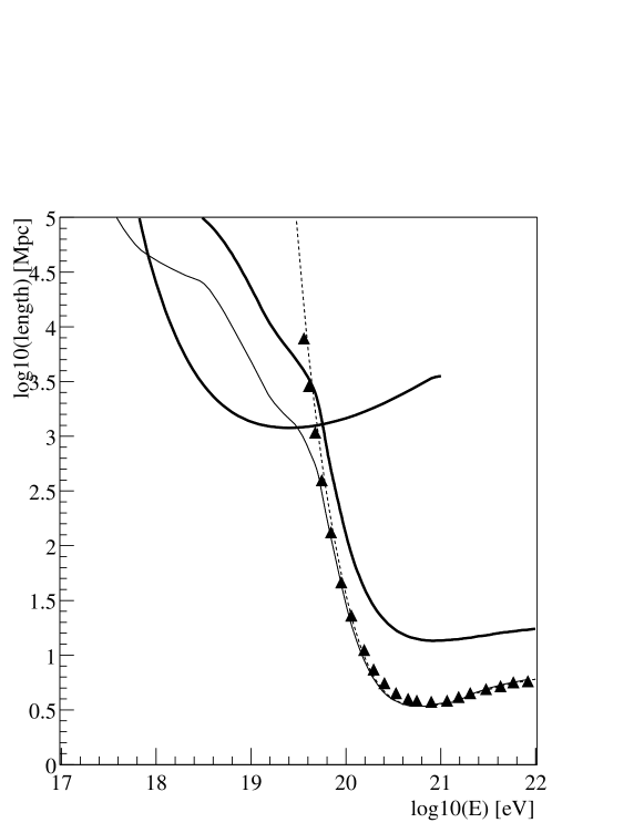
Figure 1: Interaction length for photopion production as calculated in this paper (dashed line) compared to the interaction length of [3] (solid thin line) and of [16] (triangles). The thick solid lines are the loss lengths for photopion production (on the right) and of pair production (on the left).

The simulation proceeds in the following way: a source distance is generated at random from a uniform distribution in a universe with $\Omega_{\Lambda}=0.7$ and $\Omega_{m}=0.3$. In a Euclidean universe, the flux from a source would scale as $r^{-2}$ where $r$ is the distance between the source and the observer. On the other hand, the number of sources between $r$ and $r+dr$ would scale as $r^{2}$, so that the probability that a given event has been generated by a source at distance $r$ is independent of $r$: sources at different distances have the same probability of generating any given event. In a flat universe with a cosmological constant, this is still true provided the distance $r$ is taken to be

$$r=c\int_{t_{g}}^{t_{0}}\frac{dt}{R(t)},$$ (7)

where $t_{g}$ is the age of the universe when the event was generated, $t_{0}$ is the present age of the universe, and $R(t)$ is the scale factor of the universe.

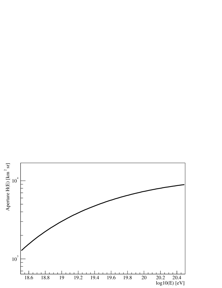
Figure 2: Aperture of the HiResI experiment as a function of the energy from [9].

Once a source distance has been selected at random, a particle energy is also assigned from a distribution that reflects the injection spectrum, chosen as in Eq. (1). This particle is then propagated to the observer and its energy recorded. This procedure is repeated until the number of events above a threshold energy, $E_{th}$ is reproduced. With this procedure we can assess the significance of results from present experiments with limited statistics of events. There is an additional complication in that the aperture of the experiment usually depends on energy. This is taken into account by allowing the event to be detected or not detected depending upon the function $H(E)$ that describes the energy dependence of the aperture.

We only study the spectrum above $10^{18.5}$ eV where the flux is supposed to be dominated by extragalactic sources. For this energy range, we focus on the experiments that have the best statistics: AGASA and HiResI. For the AGASA experiment the exposure is basically flat above $10^{19}$ eV, while for HiRes the exposure is as plotted in Fig. (2) [9]. For AGASA data, the simulation is stopped when the number of events above $E_{th}=10^{19}$ eV equals 866. For HiRes this number is 300. Note that while for AGASA the number of detected events actually corresponds to the generated events, for HiRes the number of detected events requires a correction due to the energy dependence of the aperture $H(E)$. This correction allows one to reconstruct the observed spectrum. The statistical error in the energy determination is accounted for in our simulation by generating a detection energy chosen at random from a Gaussian distribution centered at the arrival energy $E$ and with width $\Delta E/E=30\%$ for both experiments.

Our simulations reproduce well the predictions of analytical calculations, in particular at the energies where energy losses may be approximated as continuous. In Fig. 3, we compare the results of our simulation with analytical calculations carried out as in ref. [18]. The curves plotted in the figure are the so called modification factors, defined in [18, 19] for three different values of the source redshift ($z=0.002$, $z=0.02$ and $z=0.2$ from top to bottom). The differential injection spectrum is taken to be a power law $E^{-2.1}$. The points with error bars are the results of our simulations with $2\times 10^{6}$ particles produced by sources at the redshifts given above. The agreement between the simulated and analytical calculations at low energies is clear. At the energies where photo-pion production becomes important, simulations predict a slightly larger flux than analytical calculations. This is a well known result, and is due to the discreteness of photo-pion energy losses, that allow some particles to reach the detector without appreciable losses.

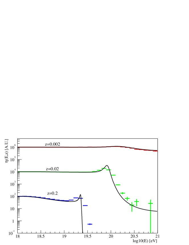
Figure 3: Comparison between analytical calculations and the results of our simulation for the modification factor, for injection spectrum $E^{-2.1}$ [18] and three values of the source redshift ($z=0.002$, $z=0.02$ and $z=0.2$ from top to bottom).

In Fig. 4 we compare the results of our simulations (points with error bars) with analytical calculations of the diffuse flux of UHECRs (continuous line) expected if sources with no luminosity evolution inject UHECRs with a spectrum $E^{-2.7}$ [20, 21]. The agreement is evident.

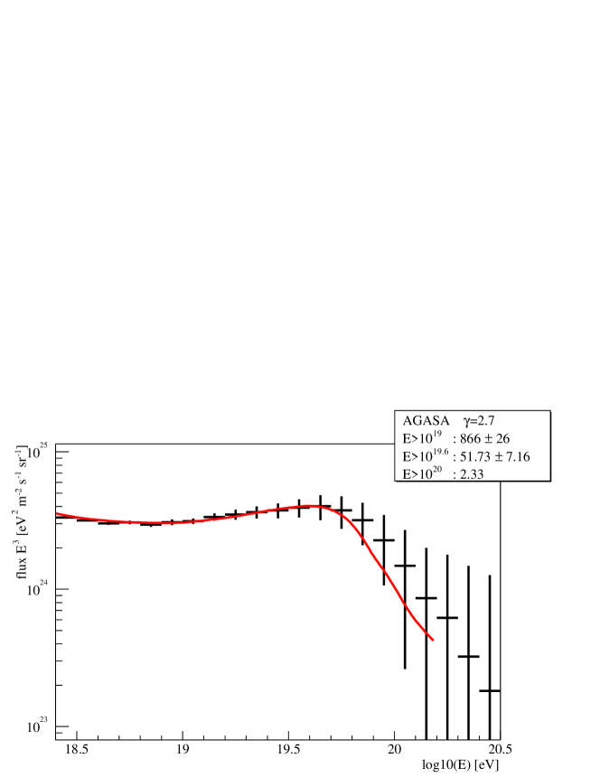
Figure 4: Comparison between the results of our simulation and the analytical calculations of [20, 21] for the case of astrophysical sources injecting cosmic rays with a spectrum $E^{-2.7}$ and no luminosity evolution.

3 AGASA versus HiResI

The two largest experiments that measured the flux of UHECRs report apparently conflicting results. The data of AGASA and HiResI on the flux of UHECRs multiplied as usual by the third power of the energy are plotted in Fig. 5 (the squares are the HiResI data while the circles are the AGASA data).

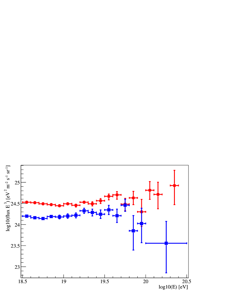
Figure 5: Circles show the AGASA spectrum from [6] while squares show the HiResI spectrum from [9].

The figure shows that HiResI data are systematically below AGASA data and that HiResI sees a suppression at $\sim 10^{20}$ eV that resembles the GZK feature while AGASA does not.

We apply our simulations here to the statistics of events of both AGASA and HiResI in order to understand whether the discrepancy is statistically significant and whether the GZK feature has indeed been detected in the cosmic ray spectrum. The number of events above $10^{19}$ eV, $10^{19.6}$ eV and $10^{20}$ eV for AGASA and HiResI are shown in Table 1. For reasons that will be clear below, we also show in the same table the number of events above the same energy thresholds, in the case that AGASA has a systematic error that overestimates the energy by $15\%$ while HiResI systematically underestimates the energy by $15\%$.

Table 1: Number of events for AGASA and HiResI detected above the energy thresholds reported in the first column.

$\log(E_{th})\,({\rm eV})$	AGASA		HiResI
	data	-15%	data	+15%
19	866	651	300	367
19.6	72	48	27	39
20	11	7	1	2.2

In order to understand the difference, if any, between AGASA and HiRes data we first determine the injection spectrum required to best fit the observations. In order to do this, we run 400 realizations of the AGASA and HiRes event statistics, as reported in the column labelled data in Table 1.

The injection spectrum is taken to be a power law with index $\gamma$ between 2.3 and 2.9 with steps of 0.1. For each injection spectrum we calculated the $\chi^{2}$ indicator (averaged over 400 realizations for each injection spectrum). The errors used for the evaluation of the $\chi^{2}$ are due to the square roots of the number of observed events. As reported in Table 2, the best fit injection spectrum can change appreciably depending on the minimum energy above which the fit is calculated. In these tables we give $\chi_{e}^{2}(N)$, where $N$ is the number of degrees of freedom, while the subscript, $e$, is the logarithm of $E_{th}$ (in eV), the energy above which the fit has been calculated. The numbers in bold-face correspond to the best fit injection spectrum. These fits are dominated by the low energy data rather than by the poorer statistics at the higher energies.

Table 2: $\chi^{2}$ for fits to AGASA and HiResI data above $10^{18.5}$ eV, $10^{19}$ eV, and $10^{19.6}$ eV for varying spectral index $\gamma$. In parenthesis the number of degrees of freedom.

	AGASA			HiResI
$\gamma$	$\chi^{2}_{18.5}(17)$	$\chi^{2}_{19}(12)$	$\chi^{2}_{19.6}(6)$	$\chi^{2}_{18.5}(15)$	$\chi^{2}_{19}(10)$	$\chi^{2}_{19.6}(4)$
2.3	1694	34	17	145	29	23
2.4	1215	24	12	80	19	15
2.5	724	19	10	36	14	11
2.6	248	16	10	14	9	7
2.7	82	17	11	33	7	5
2.8	80	21	13	126	7	4
2.9	316	27	15	257	9	4

If the data at energies above $10^{18.5}$ eV are taken into account for both experiments, the best fit spectra are $E^{-2.8}$ for AGASA and $E^{-2.6}$ for HiRes. If the data at energies above $10^{19}$ eV are used for the fit, the best fit injection spectrum is $E^{-2.6}$ for AGASA and between $E^{-2.7}$ and $E^{-2.8}$ for HiRes. If the fit is carried out on the highest energy data ($E>10^{19.6}$ eV), AGASA prefers an injection spectrum between $E^{-2.5}$ and $E^{-2.6}$, while $E^{-2.8}$ or $E^{-2.9}$ fit better the HiRes data in the same energy region. Note that the two sets of data uncorrected for any possible systematic errors require different injection spectra that change with $E_{th}$.

Table 3: Number of events expected above $E_{th}$(eV) for different injection spectra assuming the AGASA statistics above $10^{19}$ eV. In parenthesis are the number of standard deviations, $\sigma$, between the observed and expected number of events. In square brackets are the discrepancies calculated with a combined error bar of simulation and observation uncertainties, $\sigma_{tot}$.

${E_{th}}$	$\gamma=2.5$	$\gamma=2.6$	$\gamma=2.8$
$10^{19.6}$	$65\pm 8.2\,(+0.5)\,$$[+0.3]$	$58\pm 7.6\,(+1.4)\,$$[+1.0]$	$46\pm 6.8\,(+2.8)\,$$[+2.2]$
$10^{20}$	$3.5\pm 1.9\,(+2.4)\,$$[+2.1]$	$2.8\pm 1.7\,(+2.6)\,$$[+2.3]$	$2.0\pm 1.4\,(+2.8)\,$$[+2.6]$

Table 4: Number of events expected above $E_{th}$(eV) for different injection spectra assuming the HiResI statistics above $10^{19}$ eV from Table 1. In parenthesis are the number of $\sigma$ between the observed and expected number of events. In square brackets are the number of $\sigma_{tot}$.

${E_{th}}$	$\gamma=2.6$	$\gamma=2.7$	$\gamma=2.8$
$10^{19.6}$	$31\pm 5.6\,(-0.8)\,$$[-0.6]$	$28\pm 5.3\,(-0.2)\,$$[-0.1]$	$26\pm 5.2\,(+0.3)\,$$[+0.2]$
$10^{20}$	$1.9\pm 1.4\,(-0.9)\,$$[-0.5]$	$1.5\pm 1.2\,(-0.5)\,$$[-0.3]$	$1.3\pm 1.2\,(-0.3)\,$$[-0.2]$

In order to quantify the significance of the detection or lack of the GZK flux suppression, we report in Tables 3 and 4 the mean number of events above the indicated energy threshold, $\langle N(E>E_{th})\rangle$, for different injection specta. In parenthesis , we show the discrepancy between the observations as in Table 1 and the simulations in number of standard deviations, $\sigma$, where $\sigma^{2}=\langle{N(E>E_{th})^{2}-\langle N(E>E_{th})\rangle^{2}}\rangle$. From Tables 3 and 4 we can see that while HiResI is consistent with the existence of the GZK feature in the spectrum of UHECRs, AGASA detects an increase in flux, but only at the $\sim 2.5\sigma$ level for the best fit injection spectra.

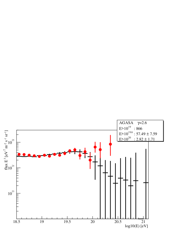
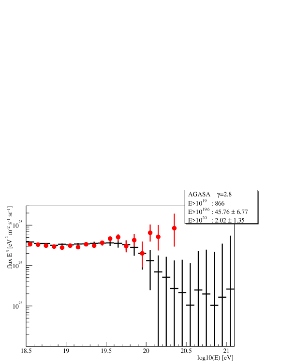
Figure 6: Simulations of AGASA statistics with injection spectra $E^{-2.6}$ (upper plot) and $E^{-2.8}$ (lower plot). The crosses with error bars are the results of simulations, while the grey points are the AGASA data.

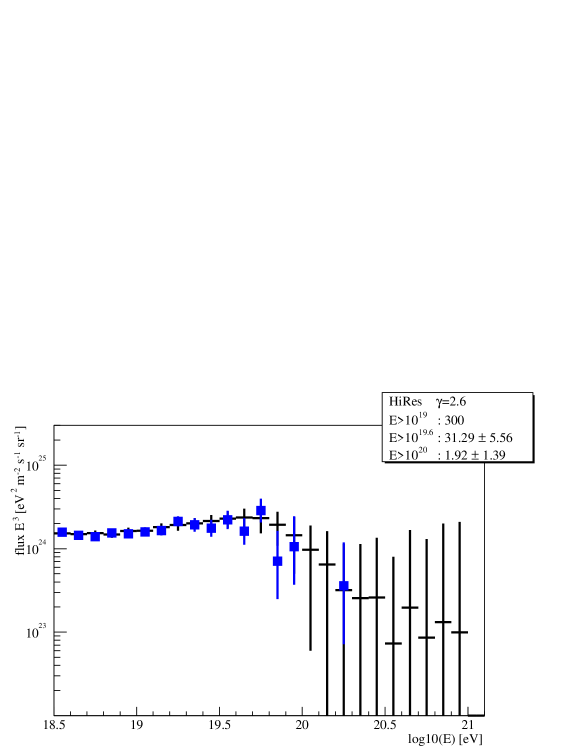
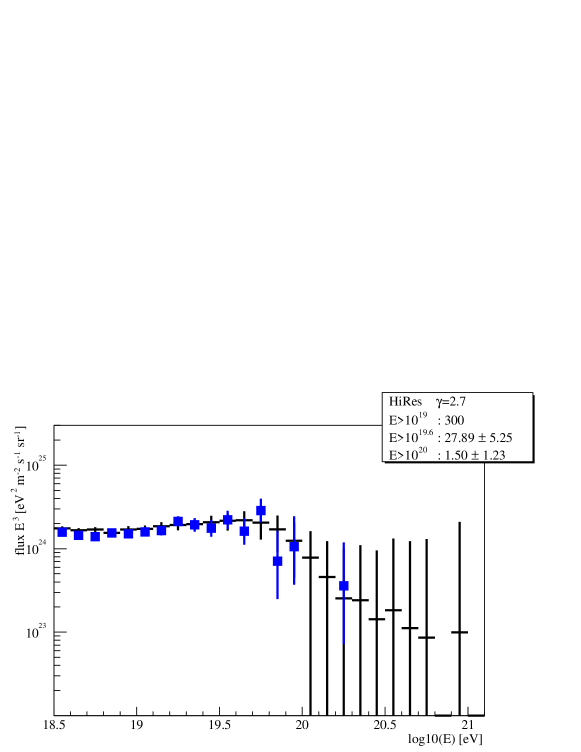
Figure 7: Simulations of HiRes statistics with injection spectra $E^{-2.6}$ (upper plot) and $E^{-2.7}$ (lower plot). The crosses with error bars are the results of simulations, while the squares are the HiRes data.

A more graphical representation of the uncertainties involved are displayed in Figs. 6 for AGASA and 7 for HiRes, for two choices of the injection spectrum. These plots show clearly the low level of significance that the detections above $E_{GZK}$ have with low statistics. The large error bars that are generated by our simulations at the high energy end of the spectrum are mainly due to the stochastic nature of the process of photo-pion production: in some realizations some energy bins are populated by a few events, while in others the few particles in the same energy bin do not produce a pion and get to the observer unaffected. The large fluctuations are unavoidable with the extremely small statistics available with present experiments. On the other hand, the error bars at lower energies are minuscule, so that the two data sets (AGASA and HiResI) cannot be considered to be two different realizations of the same phenomenon. Instead, systematic errors in at least one if not both experiments are needed to explain the discrepancies at lower energies.

Taking into account the (theoretical) error bars in the analysis makes the significance of the presence or absence of the GZK feature much weaker than the consistency checks shown in Tables 3 and 4. In order to estimate this effect, we proceed in the following way: we calculate the expected number of events above some threshold with its corresponding standard deviation ($\sigma_{sim}$), as determined by the fluctuations in the flux simulation. The observed number of events above the same threshold is also known with the error bar $\sigma_{obs}$. The discrepancy between the two is now calculated using the error $\sigma_{tot}=(\sigma_{sim}^{2}+\sigma_{obs}^{2})^{1/2}$. Our results are summarized in Tables 3 for AGASA and 4 for HiRes. The numbers with error bars are the simulated expectations, while the discrepancy between simulations and observations, calculated as described above is in square brackets, in units of $\sigma_{tot}$. It becomes clear that the effective discrepancy between predictions and the AGASA data is at the level of $2.1-2.5\sigma$. Therefore a definite answer to the question of whether the GZK feature is there or not awaits a significant improvement in statistics at high energies.

As seen in Fig. 5, the difference between the AGASA and HiResI spectra is not only in the presence or absence of the GZK feature: the two spectra, when multiplied by $E^{3}$, are systematically shifted by about a factor of two. This shift suggests that there may be a systematic error either in the energy or the flux determination of at least one of the two experiments. Possible systematic effects have been discussed in [22] for the AGASA collaboration and in [9] for HiResI. At the lower end of the energy range the offset may be due to the notoriously difficult determination of the AGASA aperture at threshold while the discrepancies at the highest energies is unclear at the moment. In any case, a systematic error of $\sim 15\%$ in the energy determination is well within the limits that are allowed by the analysis of systematic errors carried out by both collaborations.

In order to illustrate the difficulty in determining the existence of the GZK feature in the observed data in the presence of systematic errors, we split the energy gap by assuming that the energies as determined by the AGASA collaboration are overestimated by $15\%$, while the HiRes energies are underestimated by the same factor. The number of events above an energy threshold is again reported in Table 1, in the column labelled $15\%$. In this case the total number of events above $10^{19}$ eV is reduced for AGASA from 866 to 651, while for HiResI it is enhanced from 300 to 367. We ran our simulations with these new numbers of events and repeat the statistical analysis described above. The values of $\chi^{2}$ obtained in this case are reported in Table 5.

Table 5: $\chi^{2}$ for AGASA and HiResI in which a correction for a systematic $15\%$ overestimate of the energies has been assumed for AGASA and a $15\%$ underestimate of the energies has been assumed for HiResI.

	AGASA			HiResI
$\gamma$	$\chi^{2}_{18.6}(15)$	$\chi^{2}_{19}(11)$	$\chi^{2}_{19.6}(5)$	$\chi^{2}_{18.6}(14)$	$\chi^{2}_{19}(10)$	$\chi^{2}_{19.6}(4)$
2.3	505	18	12	79	13	7
2.4	351	13	8.5	40	7	4
2.5	188	9	5.6	13	3.7	2.0
2.6	54	9	5.6	6	2.0	1.1
2.7	20	11	6.4	23	3.1	1.4
2.8	54	15	7.2	94	6	2.4
2.9	145	20	9.1	176	10	4

For AGASA, the best fit injection spectrum is now between $E^{-2.5}$ and $E^{-2.6}$ above $10^{19}$ eV and above $10^{19.6}$ eV (the $\chi^{2}$ values are identical). For the HiRes data, the best fit injection spectrum is $E^{-2.6}$ for the whole set of data, independent of the threshold. It is interesting to note that the best fit injection spectrum appears much more stable after the correction of the $15\%$ systematics has been carried out. Moreover, the best fit injection spectra as derived for each experiment independently coincides for the corrected data unlike the uncorrected case. This suggests that combined systematic errors in the energy determination at the $\sim$ 30% level may in fact be present.

The expected numbers of events with energy above $10^{19.6}$ eV and above $10^{20}$ eV with the deviation from the data are reported in Tables 6 and 7: while HiResI data remain in agreement with the prediction of a GZK feature, the AGASA data seem to depart from such prediction but only at the level of $\sim 1.8\sigma$. The systematics in the energy determination further decreased the significance of the GZK feature, such that the AGASA and HiResI data are in fact only less than $2\sigma$ away from each other.

Table 6: Number of events expected above $E_{th}$ (eV) for AGASA energies decreased systematically by $15\%$. In parenthesis is the number of standard deviations between observations and simulations, $\sigma$. In square brackets are the discrepancies calculated in units of $\sigma_{tot}$.

${E_{th}}$	$\gamma=2.5$	$\gamma=2.6$	$\gamma=2.7$
$10^{19.6}$	$49\pm 6.9\,(+0.2)\,$$[+0.1]$	$43\pm 6.5\,(+0.8)\,$$[+0.5]$	$39\pm 6.1\,(+1.3)\,$$[+1.0]$
$10^{20}$	$2.6\pm 1.6\,(+1.7)\,$$[+1.4]$	$2.3\pm 1.5\,(+1.8)\,$$[+1.5]$	$1.8\pm 1.4\,(+2.0)\,$$[+1.7]$

Table 7: Number of events expected above $E_{th}$ (eV) for HiResI energies increased systematically by $15\%$. In parenthesis is the number of standard deviations between observations and simulations, $\sigma$. In square brackets are the discrepancies calculated in units of $\sigma_{tot}$.

${E_{th}}$	$\gamma=2.5$	$\gamma=2.6$
$10^{19.6}$	$43\pm 6.3\,(-0.6)\,$$[-0.4]$	$38\pm 6.0\,(+0.1)\,$$[+0.1]$
$10^{20}$	$2.8\pm 1.7\,(-0.4)\,$$[-0.3]$	$2.3\pm 1.5\,(-0.1)\,$$[-0.1]$

We can use the same procedure illustrated above to evaluate the effect of the error bars in the simulated data compared to the data corrected by 15%. The results are reported in square brackets in Tables 6 (for AGASA) and 7 (for HiRes), showing that the effective discrepancy between expectations (with uncertainties due to discrete energy losses and cosmic variance) and AGASA data is even smaller, only at the $1.5\sigma$ level. In Fig. 8, we plot the simulated spectra for injection spectrum $E^{-2.6}$ and compare them to observations of AGASA (upper plot) and HiRes (lower plot).

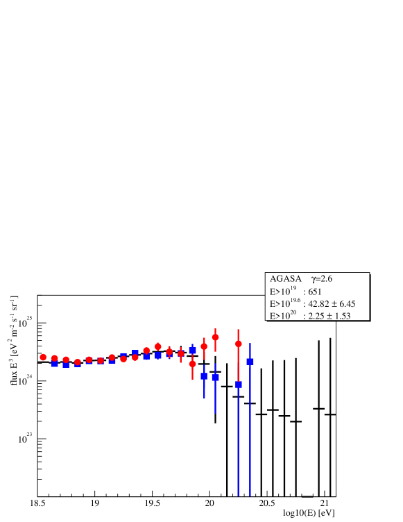
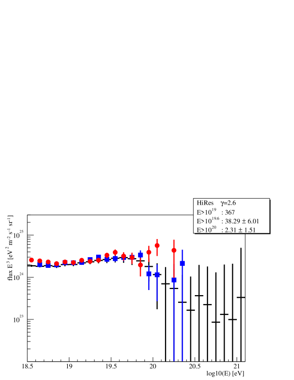
Figure 8: Simulated spectra for the best fit injection spectrum with $\gamma=2.6$. Upper panel shows simulations for the AGASA event statistics after correcting for energy by an overall shift of -15%. The lower panel shows the fluctuations expected for the event statistics of HiResI after shifting HiResI energies by +15%. The shifted data for AGASA (grey circles) and HiResI (dark squares) are shown in both panels.

4 Conclusions

We considered the statistical significance of the UHECR spectra measured by the two largest experiments in operation, AGASA and HiRes. The spectrum released by the HiResI collaboration seems to suggest the presence of a GZK feature. This has generated claims that the GZK cutoff has been detected, reinforced by data from older experiments [23]. However, no evidence for such a feature has been found in the AGASA experiment. We compared the data with theoretical predictions for the propagation of UHECRs on cosmological distances with the help of numerical simulations. We find that the very low statistics of the presently available data hinders any statistically significant claim for either detection or the lack of the GZK feature.

A comparison of the spectra obtained from AGASA and HiResI shows a systematic shift of the two data sets, which may be interpreted as a systematic error in the relative energy determination of about $30\%$. If no correction for this systematic shift is carried out, the AGASA data are best fit by an injection spectrum $E^{-\gamma}$ with $\gamma=2.6$ for energies above $10^{19}$ eV. The fit steepens to $\gamma=2.8$ when considering events down to $10^{18.5}$ eV. For HiResI, the best fit is between $\gamma=2.7$ and $\gamma=2.8$ for events with energy above $10^{19}$ eV and $\gamma=2.6$ for events above $10^{18.5}$ eV. With these best fits to the injection spectrum the AGASA data depart from the prediction of a GZK feature by $2.6\sigma$ for $\gamma=2.6$. The HiRes data are fully compatible with the prediction of a GZK feature in the cosmic ray spectrum. The fit to the data with energy above $10^{19}$ eV is probably less susceptible to contamination by a possible galactic flux. In this case the AGASA departure from the expected GZK feature is, as stressed above, at the level of about $2.6\sigma$. Taking into account the uncertainties derived from the simulations, attributed to the discreteness of the photo-pion production and to cosmic variance, this discrepancy becomes even less significant ($\sim 2.3\sigma$). It is clear that, if confirmed by future experiments with much larger statistics, the increase in flux relative to the GZK prediction hinted by AGASA would be of great interest. This may signal the presence of a new component at the highest energies that compensates for the expected suppression due to photo-pion production, or the effect of new physics in particle interactions (for instance the violation of Lorentz invariance or new neutrino interactions).

Identifying the cause of the systematic energy and/or flux shift between the AGASA and the HiRes spectra is crucial for understanding the nature of UHECRs. This discrepancy has stimulated a number of efforts to search for the source of these systematic errors including the construction of hybrid detectors, such as Auger, that utilize both ground arrays and fluorescence detectors. A possible overestimate of the AGASA energies by $15\%$ and a corresponding underestimate of the HiRes energies by the same amount would in fact bring the two data sets in agreement in the region of energies below $10^{20}$ eV. In this case both experiments are consistent with a GZK feature with large error bars. The AGASA excess is at the level of $1.7\sigma$ ($1.4\sigma$ if the observational uncertainties are also taken into account). Interestingly enough, the correction by $15\%$ in the error determination implies that the best fit injection spectrum becomes basically the same for both experiments ($E^{-2.6}$).

With the low statistical significance of either the excess flux seen by AGASA or the discrepancies between AGASA and HiResI, it is inaccurate to claim either the detection of the GZK feature or the extension of the UHECR spectrum beyond $E_{GZK}$ at this point in time. A new generation of experiments is needed to finally give a clear answer to this question. In Fig. 9 we report the simulated spectra that should be achieved in 3 years of operation of Auger (upper panel) and EUSO (lower panel). The error bars reflect the fluctuations expected in these high statistics experiments for the case of injection spectrum $E^{-2.6}$. (Note that the energy threshold for detection by EUSO is not yet clear.) It is clear that the energy region where statistical fluctuations dominate the spectrum is moved to $\sim 10^{20.6}$ eV for Auger, allowing a clear identification of the GZK feature. The fluctuations dominated region stands beyond $10^{21}$ eV for EUSO.

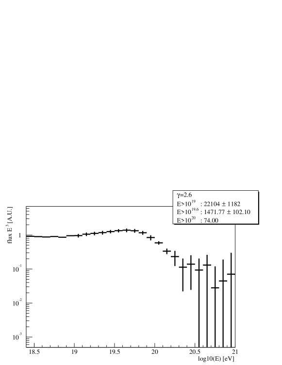
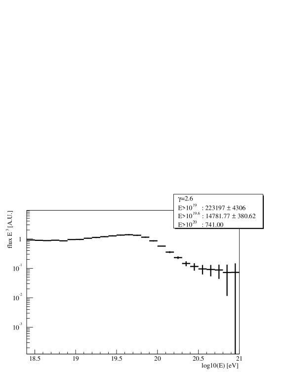
Figure 9: Predicted spectra and error bars for 3 years of operation of Auger (upper plot) and EUSO (lower plot).

References

- [1] K. Greisen, Phys. Rev. Lett. 16 (1966) 748; G. T. Zatsepin and V. A. Kuzmin, Sov. Phys. JETP Lett. 4 (1966) 78
- [2] V.S. Berezinsky, P.Blasi and A. Vilenkin, 58 (1998) 103515
- [3] P. Bhattacharjee and G. Sigl, Phys. Rept. 327 (2000) 109
- [4] A. Olinto, Phys. Rep. 333 (2000) 329
- [5] A.A. Watson, Phys. Rep., 333 (2000) 309
- [6] M. Takeda et al., Phys. Rev. Lett. 81 (1998) 1163; M. Takeda et al. preprint astro-ph/9902239 N. Hayashida et al. Phys. Rev. Lett. 73 (1994) 3491; D. J. Bird et al. Astrophys J. 441 (1995) 144; Phys. Rev. Lett. 71 (1993) 3401; Astrophys. J. 424 (1994) 491; M. A. Lawrence, R. J. O. Reid and A. A. Watson, J. Phys. G. Nucl. Part. Phys. 17 (1991) 773; N. N. Efimov et al., Ref. Proc. International Symposium on Astrophysical Aspects of the Most Energetic Cosmic Rays, eds. M. Nagano and F. Takahara (World Scientific, Singapore, 1991), p. 20
- [7] S. C. Corbató et al., Nucl. Phys. B (Proc. Suppl.) 28B (1992) 36
- [8] T. Abu-Zayyad, et al., preprint astro-ph/0208301
- [9] T. Abu-Zayyad, et al., preprint astro-ph/0208243
- [10] J. W. Cronin, Proceedings of ICRC 2001 (2001).
- [11] see http://www.euso-mission.org
- [12] R. E. Streitmatter, Proc. of Workshop on Observing Giant Cosmic Ray Air Showers from eV Particles from Space, eds. J. F. Krizmanic, J. F. Ormes, and R. E. Streitmatter (AIP Conference Proceedings 433, 1997).
- [13] M. Blanton, P. Blasi and A. V. Olinto, Astropart. Phys. 15 (2001) 275
- [14] G. R. Blumenthal, Phys. Rev. D1 (1970) 1596.
- [15] M. J. Chodorowski, A. A. Zdziarski, and M. Sikora, Astrophys. J. 400 (1992) 181.
- [16] T. Stanev, R. Engel, A. Mucke, R. J. Protheroe and J. P. Rachen, Phys. Rev. D 62 (2000) 093005.
- [17] D.E. Groom et al., The European Physical Journal C15 (2000) 1. http://pdg.lbl.gov/~sbl/gammap_total.dat
- [18] V. Berezinsky and S. Grigorieva, Astron. Astroph. 199 (1988) 1
- [19] V. S. Berezinsky, S.V. Bulanov, V. A. Dogiel, V. L. Ginzburg, and V. S. Ptuskin, Astrophysics of Cosmic Rays, (Amsterdam: North Holland, 1990)
- [20] V. Berezinsky, A. Z. Gazizov and S. Grigorieva, preprint astro-ph/0210095
- [21] V. Berezinsky, A. Z. Gazizov and S. Grigorieva, preprint hep-ph/0204357.
- [22] M. Takeda et al., preprint astro-ph/0209422
- [23] J.N. Bahcall and E. Waxman, preprint hep-ph/0206217