The Oort Constants Measured from Proper Motions

Abstract

The Oort constants describe the local spatial variations of the stellar streaming field. The classic way for their determination employs their effect on stellar proper motions. We discuss various problems arising in this procedure. A large, hitherto apparently overlooked, source of potential systematic error arises from longitudinal variations of the mean stellar parallax, caused by intrinsic density inhomogeneities and inter-stellar extinction. Together with the reflex of the solar motion these variations by mode mixing create contributions to the longitudinal proper motions ${\overline{\mu}}_{\ell^{\star}}(\ell)$ that are indistinguishable from the Oort constants at $\lesssim 20\%$ of their amplitude. Fortunately, we can correct for this mode mixing using the latitudinal proper motions $\mu_{b}(\ell)$.

We use about 10⁶ stars from the ACT/Tycho-2 catalogs brighter than $V\approx 11$ with median proper motion error of $\approx 3\,\mbox{${\rm mas}\,{\rm yr}^{-1}$}$. Taking every precaution to avoid or correct for the various sources of systematic error, significant deviations from expectations based on a smooth axisymmetric equilibrium, in particular non-zero $C$ for old red giant stars. We also find variations of the Oort constants with the mean color, which correlate nicely with the asymmetric drift of the sub-sample considered. Also these correlations are different in nature than those expected for an axisymmetric Galaxy.

The most reliable tracers for the “true” Oort constants are red giants, which are old enough to be in equilibrium and distant enough to be unaffected by possible local anomalies. For these stars we find, after correction for mode-mixing and the asymmetric drift effects, $A\approx 16$, $B\approx-17$, $A-B\approx 33$, and $C\approx-10$ ${\rm km}\,{\rm s}^{-1}\,{\rm kpc}^{-1}$with internal errors of about 1-2 and external error of perhaps the same order. These values are consistent with our knowledge of the Milky Way (flat rotation curve and $\Omega\equiv A-B\approx 28\pm 2$). Based on observations made with the ESA Hipparcos astrometry satellite.

1 Introduction

For over eight decades, the distribution and kinematics of stars in the solar neighborhood has been studied in order to infer the structure of the Milky Way galaxy. Kapteyn & van Rhijn (1920) used star counts to determine the size and thickness of the Milky Way. Furthermore, by assuming hydrostatic equilibrium perpendicular to the Galactic plane, the radial velocities and proper motions of nearby stars allowed Kapteyn (1922) to make the first reasonable estimate of the mass of the Milky Way. However, Oort (1927a) pointed out that the mass of Kapteyn’s Galaxy is not large enough to keep the globular clusters and RR Lyrae stars bound to the Galaxy. Lindblad (1927) proposed that the sub-systems of high-velocity stars and globular clusters as well as that of nearby low-velocity stars have the same axis of symmetry and a common center – that of the globular clusters (Shapley, 1918). Lindblad further hypothesized that each of these sub-systems is in dynamical equilibrium, and that the sub-systems with the largest amount of rotation will have the flattest space distribution and the smallest peculiar velocities (Jeans, 1922), in agreement with the then available data.

The motions of the stars in the solar neighborhood can be interpreted as a streaming (average) velocity plus random motions. In disk galaxies, the first dominates over the second: such stellar systems are said to be dynamically cold. In the solar neighborhood, for instance, the velocity dispersion in the plane, i.e. the amplitude of random motions, is 45 ${\rm km}\,{\rm s}^{-1}$ for the old stellar disk and 18 ${\rm km}\,{\rm s}^{-1}$ for early-type stars, while the streaming motion is of the order of 200 ${\rm km}\,{\rm s}^{-1}$. In the cold limit of vanishing random motions, the streaming is along the closed orbits supported by the gravitational potential. Thus, knowledge about the potential of the Milky Way, and hence its mass distribution, can be gained from studies of the stellar streaming velocities.

Oort laid the theoretical basis of this method with his pioneering paper (1927a). To begin with, let us follow Oort and consider the cold limit in which all stars move on closed orbits. Oort himself actually considered the Milky way to be axisymmetric, but his analysis is easily generalized to non-axisymmetry (Ogorodnikov, 1932; Milne, 1935; Chandrasekhar, 1942). At each position ${\boldsymbol{x}}$ in the Galaxy, there is a unique streaming velocity ${\boldsymbol{v}}$ (here, we ignore the possibility of orbit crossing). The difference $\delta{\boldsymbol{v}}$ between the velocity at some point in the Galaxy and that at the Sun may be expanded in a Taylor series (with local Cartesian coordinates: $\hat{{\boldsymbol{e}}}_{x}$ and $\hat{{\boldsymbol{e}}}_{y}$ pointing in directions $\ell=0\arcdeg$ and $\ell=90\arcdeg$)

$$\delta{\boldsymbol{v}}=\mathbf{H}\cdot{\boldsymbol{x}}+{\cal O}({\boldsymbol{x}}^{2})$$ (1)

with

$$\mathbf{H}=\left(\begin{array}[]{c@{\;\;}c}\partial v_{x}/\partial x&\partial v_{y}/\partial x\\ \partial v_{x}/\partial y&\partial v_{y}/\partial y\end{array}\right)_{{\boldsymbol{\scriptstyle x}}=0}\equiv\left(\begin{array}[]{c@{\;\;}c}K+C&A-B\\ A+B&K-C\end{array}\right).$$ (2)

The parameters $A$, $B$, $C$, and $K$ are the Oort constants, they measure the local divergence ($K$), vorticity ($B$), azimuthal ($A$) and radial ($C$) shear of the velocity field generated by closed orbits. A star at Galactic longitude $\ell$ and distance $d$ from an observer and moving with velocity ${\boldsymbol{v}}$ relative to the latter, is observed to have radial and tangential velocity

$$v_{d} = \phantom{string}v_{x}\cos\ell+v_{y}\sin\ell$$ (3a)

$$v_{\ell} = -v_{x}\sin\ell+v_{y}\cos\ell.$$ (3b)

Inserting equation (1) with ${\boldsymbol{x}}=d(\cos\ell,\sin\ell),$ whereby assuming the observer participates in the streaming field, one finds

$$v_{d}\,d^{-1} = K+A\sin 2\ell+C\cos 2\ell+\mathcal{O}([d/R_{0}]^{2})$$ (4a)

$$v_{\ell}\,d^{-1} = B-C\sin 2\ell+A\cos 2\ell+\mathcal{O}([d/R_{0}]^{2}).$$ (4b)

It is worth emphasizing that terms quadratic in $d/R_{0}$ contribute to the $m=\pm 1,3$ harmonics $\mathrm{e}^{im\ell}$ in equation (4) and thus do not interfere with the Oort constants – however, terms of higher odd orders do. Similarly, the deviations of the solar velocity from the local streaming velocity leads to $m=\pm 1$ harmonics, see below.

The Oort constants may also be expressed in terms of cylindrical coordinates $(R,\varphi)$ with the Sun at $(R_{0},0)$ (cf. Chandrasekhar 1942)

$$2A = \phantom{string}\frac{v_{\varphi}}{R}-\frac{\partial v_{\varphi}}{\partial R}-\frac{1}{R}\frac{\partial v_{R}}{\partial\varphi},$$ (5a)

$$2B = -\frac{v_{\varphi}}{R}-\frac{\partial v_{\varphi}}{\partial R}+\frac{1}{R}\frac{\partial v_{R}}{\partial\varphi},$$ (5b)

$$2C = -\frac{v_{R}}{R}+\frac{\partial v_{R}}{\partial R}-\frac{1}{R}\frac{\partial v_{\varphi}}{\partial\varphi},$$ (5c)

$$2K = \phantom{string}\frac{v_{R}}{R}+\frac{\partial v_{R}}{\partial R}+\frac{1}{R}\frac{\partial v_{\varphi}}{\partial\varphi}$$ (5d)

evaluated at the solar position (we use the convention that $\varphi$ increases clockwise, i.e. in the direction of Galactic rotation). In the axisymmetric limit, $C=K=0$, and

$$A_{\rm sym} = \frac{1}{2}\left(\phantom{string}\frac{v_{\varphi}}{R}-\frac{\partial v_{\varphi}}{\partial R}\right)_{R=R_{0}},$$ (6a)

$$B_{\rm sym} = \frac{1}{2}\left(-\frac{v_{\varphi}}{R}-\frac{\partial v_{\varphi}}{\partial R}\right)_{R=R_{0}},$$ (6b)

equivalent to the equations actually given by Oort. In an axisymmetric Galaxy, the circular (closed) orbits have velocity $v_{\varphi}^{2}=R\;\partial\Phi/\partial R$, and measurements of the Oort constants provide a direct constraint on the Galactic potential $\Phi$. For instance, a harmonic potential results in solid-body rotation, $A=0$, and $B$ equal to the (constant) rotation frequency, a flat rotation curve gives $A={-}B$, and the case of all the mass concentrated in the inner Galaxy yields $A={-}3B$. From the then available radial velocities and proper motions, Oort (1927b) found $A\approx 19\,\mbox{${\rm km}\,{\rm s}^{-1}\,{\rm kpc}^{-1}$}$ and $B\approx-24\,\mbox{${\rm km}\,{\rm s}^{-1}\,{\rm kpc}^{-1}$}$ (with large uncertainties, though). This was clear evidence for a rotation of the Milky Way (not well established at that time), and ruled out Lindblad’s suggestion that the Milky Way rotates like a solid body. Note, however, that zero $C$ and $K$ do not necessarily imply axisymmetry of the Galactic potential; alternatively, the Sun might be located near a principal axis of an elliptic potential (Kuijken & Tremaine, 1994).

Given their pre-eminent importance, it should not come as a surprise that the observational determination of the Oort constants has been high on the astronomers’ priority list. However, measuring these streaming velocities directly is no simple task, mainly because of the lack of an appropriate reference system which is unaffected by systematic motions and not involved in the Galactic streaming. For example, stellar positions and proper motions in the fundamental stellar catalogs (e.g. AGK3, FK4, FK5) are based on transit time measurements. The so-determined proper motions are absolute, but with respect to a reference frame tied to the Earth and the orbits of Solar system objects, and are thus useful to determine Earth’s precession rate and the motion of the equinox (e.g., Fricke, 1971; Clube, 1972; Miyamoto & Soma, 1993; Lindgren & Kovalevsky, 1995). In order determine the Galactic rotation rate, it is more useful to determine proper motions relative to an extra-galactic inertial reference frame. In more modern proper motion programs, distant galaxies have been used for this purpose (e.g., NPM, SPM, KSZ, Bonn, Potsdam, see Kovalevsky et al., 1997, for a summary). However, until recently their usefulness has been limited by the so-called “magnitude equation” problem. Comparison with the Hipparcos data showed that several of these extra-galactic reference frames were not exactly inertial. Some significant residual spins (0.25 - 1.25 mas yr^-1) of the pre-Hipparcos coordinate systems were found (see Kovalevsky et al., 1997, for a review), which can lead to systematic errors in the Oort constant $B$ of 1.2-6 ${\rm km}\,{\rm s}^{-1}\,{\rm kpc}^{-1}$.

So far, we have only considered the cold limit and ignored the effect of random motions. However, we will see that this is not suitable for most stars in the solar neighborhood. That is, the mean velocity field of a group of stars differs systematically and significantly in its divergence, vorticity and shear from the (hypothetical) velocity field induced by closed orbits. Moreover, higher-order terms in the Taylor expansion and other effects imply that the Fourier coefficients in equation (4) are not identical to the divergence, vorticity, and shear of the mean velocity field, let alone the closed-orbit velocity field. These problems (discussed in some detail in §2 with particular emphasize on proper-motion data) introduce significant systematic errors in the values derived for the Oort constants. In most previous studies, many of these problems have been ignored, a fact that may well explain the diversity among the values derived for the Oort constants from different data and by different methods (see Kerr & Lynden-Bell, 1986; Olling & Merrifield, 1998, for reviews). The main objective of the present paper is, after having recognized these systematic errors, to avoid them as far as possible both by a careful analysis of the data and a careful interpretation of the results. §3 details our analysis technique. In §4, we motivate our selection of the ACT catalog and analyze its proper motion data. The results are discussed and interpreted in §5. Finally, §6 sums up and concludes.

For the convenience of authors and readers, the units used throughout this paper will be consistent and will not always be explicitly given. Distances are measured in ${\rm kpc}$, velocities in ${\rm km}\,{\rm s}^{-1}$, and frequencies, such as proper motions and the Oort constants, in ${\rm km}\,{\rm s}^{-1}\,{\rm kpc}^{-1}$. Stellar parallaxes, denoted by the symbol $\pi$, are considered to be inverse distances and, consequently, have dimension ${\rm kpc}$^-1, which corresponds to measuring the actual parallax angle in milli-arcseconds. Luminosities and colors are given in magnitudes as usual.

2 The Oort Constants in Practice

2.1 Deviations from the Cold Limit

As already pointed out by Oort (1928) and later discussed by Kuijken & Tremaine (1994), only in the cold limit of vanishing random motions can we interpret the mean streaming velocity ${\overline{{\boldsymbol{v}}}}$ as the velocity ${\boldsymbol{v}}$ of closed orbits supported by the Galactic potential. In general, there is a systematic difference, and we may write

$${\overline{{\boldsymbol{v}}}}={\boldsymbol{v}}-{\boldsymbol{v}}_{a}$$ (7)

with the asymmetric drift velocity ${\boldsymbol{v}}_{a}$. The asymmetric drift expresses the lag of the mean velocity with respect to the local closed orbit. To explicitly make this distinction, let us write in analogy to (7)

$${\overline{A}} = A-A_{a},$$ (8a)

$${\overline{B}} = B-B_{a},$$ (8b)

$${\overline{C}} = C-C_{a},$$ (8c)

$${\overline{K}} = K-K_{a}.$$ (8d)

Here, ${\overline{A}}$, ${\overline{B}}$, ${\overline{C}}$, and ${\overline{K}}$ represent the mean velocity field (its divergence, vorticity and shear) of a group of stars and might be evaluated from equation (2) or (5) by replacing ${\boldsymbol{v}}$ with ${\overline{{\boldsymbol{v}}}}$, while $A_{a}$, $B_{a}$ etc. follow upon replacing ${\boldsymbol{v}}$ with ${\boldsymbol{v}}_{a}$.

For an axisymmetric Galaxy, there is only an azimuthal component $v_{a\varphi}$, which, for random motions much smaller than the rotation velocity, can be approximated by Strömberg’s relation (see Binney & Tremaine, 1987, eq. 4.34, for a derivation from the Jeans equations)

$$2v_{\varphi}v_{a\varphi}\simeq\sigma_{R}^{2}\left[\frac{\sigma_{\varphi}^{2}}{\sigma_{R}^{2}}-1-\frac{\partial\ln(\rho\sigma_{R}^{2})}{\partial\ln R}-\frac{R}{\sigma_{R}^{2}}\frac{\partial\sigma_{Rz}^{2}}{\partial z}\right].$$ (9)

Here, ${\boldsymbol{\sigma}}^{2}$ is the (square of the) velocity dispersion tensor and $\rho$ the stellar density. Thus, the asymmetric drift is a function of the radial velocity dispersion but also depends on the circular velocity, the axis-ratio of the velocity dispersion ellipsoid, as well as on gradients in the dispersion and stellar density. We might use this relation to estimate the expected effect on Oort’s $A$ and $B$. We refer the reader to Lewis & Freeman (1989) for a determination of the radial dependence of the radial and tangential velocity dispersions. We proceed by neglecting the radial variation of the last term in (9) and by assuming that $\rho$ and ${\boldsymbol{\sigma}}^{2}$ vary exponentially with scale lengths $R_{d}$ and $R_{\sigma^{2}}$. We then find:

$$\frac{\partial\ln v_{a\varphi}}{\partial R}\simeq-\frac{1}{R_{\sigma^{2}}}+\frac{k}{2v_{\varphi}}\left(\frac{1}{R_{d}}{+}\frac{1}{R_{\sigma^{2}}}\right)-\frac{\partial\ln v_{\varphi}}{\partial R},$$ (10)

where we have used $k\,v_{a\varphi}\simeq\sigma_{R}^{2}$ with $k=(80\pm 5)\,\mbox{${\rm km}\,{\rm s}^{-1}$}$ (Dehnen & Binney 1998, hereafter DB98).

For $R_{\sigma^{2}}=0.45R_{0}$ (Lewis & Freeman, 1989), one finds $A_{a}\approx 0.14v_{a\varphi}$ and $B_{a}\approx 0.01v_{a\varphi}$, almost independent of $R_{d}$, $R_{0}$, and $v_{\varphi}$. That is, $B$ is hardly affected, while $A_{a}$ might be as large as 3 for red stars (using $v_{a\varphi}$ of 20 according to DB98’s findings).

This derivation of $A_{a}$ and $B_{a}$ is based on the assumption of dynamical equilibrium, and hence not appropriate for young stellar populations, whose lumpy phase-space structure (moving groups and inhomogeneous spatial distribution) indicates non-equilibrium. Further, note that the numerical values derived above from equation (10) are only valid in the Solar neighborhood as $k$ and $v_{a\varphi}$ were determined locally.

It is important to notice that ${\overline{A}}$, ${\overline{B}}$, ${\overline{C}}$, and ${\overline{K}}$ are functions of Galactic height $z$ (already because the asymmetric drift depends on $z$). One might think that one could just extend the Taylor expansion (1) into the vertical direction. However, this does not work, mainly because the scale height of the stellar disk, and hence any possible kinematic gradients, is much smaller than reasonable sample depths, i.e. high-order terms are significant. (Also, for symmetry reasons, the first non-trivial term is quadratic and its distance dependence would not nicely vanish in the resulting proper motions.)

2.2 Deviations from Axisymmetry

For an axisymmetric Galaxy, as originally considered by Oort, the closed orbits are circular and at each radius there exists exactly one such orbit. However, the Galaxy is not axisymmetric, it has a central bar and its disk appears to have 4, or a 4+2, armed spiral pattern (Vallée, 1995; Amaral & Lépine, 1997), but the infrared light, originating mainly from old stars, is dominated by a 2-arm mode (Drimmel, 2000; Drimmel & Spergel, 2001). As a consequence, the closed orbits are no longer circular but elliptical. The orientation of these elliptic orbits changes when one crosses the co-rotation or inner and outer Lindblad resonances (CR, ILR, & OLR) of the bar or spiral pattern. Certain places near these resonances are visited by two or more differently oriented closed orbits. It has even been proposed that the Sun is precisely at such a position on the OLR (Kalnajs, 1991). However, it seems now more likely from detailed models of the gaseous and stellar motions in the inner parts of the Milky Way that we are about 1 ${\rm kpc}$ or even less outside the OLR (Englmaier & Gerhard, 1999; Fux, 1999; Dehnen, 1999, 2000). The spiral pattern of the Milky Way also imposes non-axisymmetric perturbations on the velocity field (Lin, Yuan & Shu, 1969; Mishurov Pavlovskaia & Suchkov, 1979). Analyses of radial velocities and now also of proper motions of several young tracer populations indicate that the Sun is located close to the radius of co-rotations of the spiral density wave ($\Delta R=\pm 1$ kpc, $\Delta\Omega=\pm 2\,\mbox{${\rm km}\,{\rm s}^{-1}\,{\rm kpc}^{-1}$}$; Crézé & Mennessier, 1973; Amaral & Lépine, 1997; Mishurov & Zenina, 1999).

Clearly, the Oort constants, defined in terms of the closed-orbit velocity field, are ill-defined at these positions, and will behave discontinuously when crossing one of the three major resonances. Of course, in reality one measures the Oort constants from stars that are not on closed orbits. In this case, the discontinuities of the Oort constants will be replaced by a more gradual transition.

2.3 Measuring the Oort Constants

The Oort constants are measured by determining the Fourier coefficients in equation (4). However, in reality the Galaxy is not flat but three-dimensional, and we cannot use this equation directly. To generalize for stars out of the plane, we use

$$\begin{array}[]{r@{\,=\,}l}\pi&d^{-1}\,\cos b\\ v_{r}&v_{d}\,\cos b\\ {\overline{\mu}}_{\ell^{\star}}&\pi\,v_{\ell}\\ \mu_{b}&-\pi\,v_{d}\,\sin b,\end{array}$$

where $\pi$ denotes the star’s parallax, $d$ the distance projected onto the Galactic plane and ${\overline{\mu}}_{\ell^{\star}}\equiv\mu_{\ell}\,\cos b$ (the quantity actually measured in astrometry). Moreover, the Sun is not moving with the local streaming velocity but with some velocity ${\overline{{\boldsymbol{v}}}}_{\odot}\equiv({\overline{U}},{\overline{V}},{\overline{W}})$ relative to it. We thus finally have for the observable proper motions, neglecting higher-order terms in equation (1),

$${\overline{\mu}}_{\ell^{\star}} \,=\, {\overline{\mu}}_{U}\sin\ell-{\overline{\mu}}_{V}\cos\ell$$ (11a)

$$+\cos b\,(\tilde{B}-\tilde{C}\sin 2\ell+\tilde{A}\cos 2\ell)$$

$${\overline{\mu}}_{b} \,=\, \sin b\,({\overline{\mu}}_{U}\cos\ell+{\overline{\mu}}_{V}\sin\ell)-{\overline{\mu}}_{W}\cos b$$ (11b)

$$-\sin b\,\cos b\,(\tilde{K}+\tilde{A}\sin 2\ell+\tilde{C}\cos 2\ell),$$

with the reflex of the solar motion

$${\overline{{\boldsymbol{\mu}}}}_{\odot}\equiv({\overline{\mu}}_{U},{\overline{\mu}}_{V},{\overline{\mu}}_{W})\equiv\pi\,{\overline{{\boldsymbol{v}}}}_{\odot}.$$ (12)

Note that we have written $\tilde{A}$ instead of ${\overline{A}}$ etc.; the symbols with a tilde are defined by equation (11), i.e. as Fourier coefficients of the mean proper motion for stars at the same distance, while those with a bar are the divergence, vorticity, and shear of the mean velocity field for a group of stars. Strictly speaking, these are two different sets of quantities, and we can only hope that they are not too different. Of course, all we can hope to measure are $\tilde{A}$, $\tilde{B}$, $\tilde{C}$, and $\tilde{K}$, while we want ${\overline{A}}$, ${\overline{B}}$, ${\overline{C}}$, and ${\overline{K}}$ (actually, $A$, $B$, $C$, and $K$). We now discuss potential sources of discrepancies between these two sets of quantities, and further problems in measuring the Fourier coefficients.

2.4 Systematics with Sample Depth

Equations (5) are based on the first-order Taylor series (1) and neglect higher-order terms, which might become important for deep samples. Including the next order adds six new unknowns, while only the $m=$1, 3 Fourier terms in ${\overline{\mu}}_{\ell^{\star}}$ are affected, i.e. only two more constraints are available (the $\cos 3\ell$ and $\sin 3\ell$ terms). Thus, the next higher-order expansion is not generally soluble from proper motion data alone.

For illustration, we now consider the effect of a purely axisymmetric model, which adds only one additional unknown per Taylor order (Pont, Mayor & Burki, 1994; Feast & Whitelock, 1997). To next order in $d/R_{0}$, we then get at $b=0$:

$${\overline{\mu}}_{\ell^{\star}} = ({\overline{\mu}}_{\ell^{\star}})_{0}+\frac{d}{8R_{0}}\left(3R_{0}\frac{\partial^{2}v_{\varphi}}{\partial R^{2}}\Big{|}_{R_{0}}-6A\right)\cos\ell$$

$$+\frac{d}{8R_{0}}\left(R_{0}\frac{\partial^{2}v_{\varphi}}{\partial R^{2}}\Big{|}_{R_{0}}+6A\right)\cos 3\ell,$$

where $({\overline{\mu}}_{\ell^{\star}})_{0}$ refers to the expression (11a). From analyses of Cepheid kinematics, the value of $\partial^{2}v_{\varphi}/\partial R^{2}|_{R_{0}}$ is estimated to be smaller than 3 km s^-1 kpc^-2 in modulus. With this estimate and $A\approx 15$, one finds that the term ${\cal O}(x)$ contributes up to $-2.5$ and 1.8 to the $\cos\ell$ and $\cos 3\ell$ Fourier terms, respectively, for $d/R_{0}=1/8$. Thus, even for a rather smooth streaming field higher-order terms may become important already at modest sample depth.

2.5 Effects of a Non-Smooth Streaming Field

Because of local anomalies in the Galactic force field, e.g. caused by spiral arms and other distortions, the streaming field inevitably exhibits small-scale oscillations on top of an underlying smooth field. These oscillations give rise to significant higher-order terms in the Taylor expansion (1). Since in practice the Oort constants are measured from the kinematics of large stellar samples with a finite depth, these high-order terms become important. In the present context, however, we are predominantly interested not in the small-scale but the large-scale behavior of the streaming field. When using a deep sample, i.e. a big volume, one might hope that the small-scale wiggles average out and one is left with the Oort constants due to the smooth equilibrium field.

Figure 1: Effect of a wiggly streaming velocity on the measured Oort’s constants. The curved (black) line in (a) represents an axisymmetric model for the streaming (rotation) velocity. From the exact $\mu_{\ell}(\ell,d)$ predicted by this model, we have measured, as function of distance, $\tilde{A}$ and $\tilde{B}$ as Fourier coefficients (b). Recovering the rotation velocity from $\tilde{A}$ and $\tilde{B}$ obtained in this way yields the straight lines in (a). The radial extent of these lines corresponds to twice the distance.

We have simulated this effect in Figure 1, where an axisymmetric streaming velocity (black line in upper panel) with wiggles of wave-length $\lambda\approx 2\,\mbox{${\rm kpc}$}$ and amplitude of only two percent of an otherwise smooth (power-law) rotation velocity is assumed. From this model, and the exact proper motion equation

$$\mu_{\ell}(\ell,d)=\frac{{\overline{v}}_{\varphi}(R)[R_{0}\cos\ell-d]/R-{\overline{v}}_{\varphi}(R_{0})\cos\ell}{d},$$ (13)

we measured the Fourier coefficients $\tilde{A}$ and $\tilde{B}$ as function of distance $d$ (LABEL:wiggleb). Assuming that the $\tilde{A}$ and $\tilde{B}$ obtained in this way measure the local streaming field, one may approximate that locally

$${\overline{v}}_{\varphi}\simeq 2R_{0}\tilde{A}-R(\tilde{A}+\tilde{B}).$$

The straight lines in LABEL:wigglea, reaching from $R_{0}-d$ to $R_{0}+d$, represent these approximations. One finds that for nearby stars ($d\ll\lambda$) the measured Oort constants $\tilde{A}$ and $\tilde{B}$ accurately represent the (wiggly) local streaming field. For distances $d$ similar to or larger than $\lambda$, $\tilde{A}$ and $\tilde{B}$ represent the underlying smooth part. For intermediate distances, there is a transition with a range in $R_{0}(\tilde{A}-\tilde{B})$ [the estimate for ${\overline{v}}_{\varphi}(R_{0})$] comparable to twice the amplitude of the wiggles. The estimated gradient of ${\overline{v}}_{\varphi}$ (the slope of the straight [red] lines) is a strong function of $d$, giving sensible results only for $d>\lambda$.

The importance of these effects is likely to be strongest for young stars and weakest for old stars, because their larger velocity dispersion makes old stellar populations less susceptible to small-scale features in the force field. From the above it is clear that even the smallest degree of non-smoothness (2%) in the Galactic force field can have a significant effect on the apparent values of the Oort constants (30%). In fact, one can show that the degree to which a stellar population with radial dispersion $\sigma_{R}$ responds to small-scale perturbations is inversely proportional to $\sigma^{2}_{R}$ (Mayor (1974)). Thus, while young stars are ideally suited to trace Galactic fine-structure, old stars with their larger dispersion are much less influenced by any wiggles in the force field and are thus more suitable to study the large-scale potential of the Milky Way. A quantitative estimate for the critical wave-length to which a group of stars with dispersion $\sigma_{R}$ is just sensitive, may be given by the average epicycle diameter $\sqrt{8}\sigma_{R}/\kappa$. With a epicycle frequency of $\kappa\approx 36\,\mbox{${\rm km}\,{\rm s}^{-1}\,{\rm kpc}^{-1}$}$ and $\sigma_{R}$ of $\approx 15\,\mbox{${\rm km}\,{\rm s}^{-1}$}$ and $\approx 38\,\mbox{${\rm km}\,{\rm s}^{-1}$}$ for blue and red stars (DB98), we find a limiting wave-length of $\approx 1\,\mbox{${\rm kpc}$}$ and $\approx 3\,\mbox{${\rm kpc}$}$, respectively. From the structure in the interstellar medium (ISM), we expect wiggles on the scale of about 2 ${\rm kpc}$ (Olling & Merrifield, 1998), which can result in 30% “errors” in the Oort constants.

Groups of stars with a radial velocity dispersion larger than about 25 ${\rm km}\,{\rm s}^{-1}$ have an epicyclic diameter larger than the wavelength of the ISM-induced wiggle of the rotation curve. Main-sequence stars bluer than $\bv=0.42$ have dispersions smaller than 25 ${\rm km}\,{\rm s}^{-1}$ (DB98) and main-sequence lifetimes less than about 2 Gyr. Thus, the kinematics of stars younger than 2 Gyr may be significantly influenced by low-amplitude, small-scale perturbations in the Galactic potential. Non-axisymmetric perturbations –which were not considered by OM98– could lead to even larger differences between the apparent Oort constants and the “true” Oort constants.

In fact, the situation depicted in Figure 1 is likely to be a simplification. In the calculations leading to LABEL:wiggle we assumed that the Sun is located half-way between the extrema of the rotation curve wiggle. That is to say, we assumed that the Sun is located in a special place with respect to the inevitable small-scale oscillations of the Galactic force field. Olling & Merrifield’s (1998) work suggests that, indeed, the Sun is not located in a “sweet spot” of the wiggly ${\overline{v}}_{\varphi}(R)$ curve (see also Amaral et al., 1996). In that case, the widely employed technique of expanding the rotation curve and the velocity field to low-order (1) is not adequate.

And finally, since there is evidence that the Milky Way exhibits significant azimuthal asymmetry (§2.2), the arguments presented above are likely to be over-simplifications. Nevertheless, the reasoning above gives us an indication as to the level of possible systematic errors in our analyses (see also §2.8.2).

2.6 Correlations of Parallax with Kinematics

In reality, of course, the stars are not just at one distance, but distributed over the sampling volume. That is, for each $\ell$, one averages along the line of sight. In order to arrive at an equivalent to equation (11) for a sample of stars are various $\pi$, one must assume that ${\overline{\pi\,U}}={\overline{\pi}}\,{\overline{U}}$ and analogously for ${\overline{\pi\,V}}$ and ${\overline{\pi\,W}}$, i.e. that parallaxes and velocities are uncorrelated. However, for stars associated with spiral arms one expects such correlations. A systematic error is introduced when using this assumption for stellar samples for which it is not justified.

2.7 Mode Mixing

When measuring the Oort constants from proper motions, one often uses a magnitude-limited sample with little information about the stellar parallaxes. One then has to replace $\pi$ in (12) by the line-of-sight averaged parallax ${\overline{\pi}}$ (or, more precisely, $\pi{\overline{{\boldsymbol{v}}}}_{\odot}$ by ${\overline{\pi{\boldsymbol{v}}}}_{\odot}$). Due to non-uniformity both of the stellar space-density and of the extinction, ${\overline{\pi}}$ will inevitably depend on longitude. We might expand it into a Fourier series in $\ell$

$${\overline{\pi}}\equiv{\overline{\pi}}_{0}\Big{(}1+2\sum_{m}c_{\pi m}\cos m\ell+s_{\pi m}\sin m\ell\Big{)},$$ (14)

where the pre-factor of two in front of the Fourier sum has been introduced for later convenience. Inserting (14) and (12) into equation (11) gives

$$\begin{array}[]{rclcclclclcl}{\overline{\mu}}_{\ell^{\star}}&=&&(&&\tilde{B}\cos b&+&s_{\pi 1}{\overline{\mu}}_{U0}&-&c_{\pi 1}{\overline{\mu}}_{V0})\\ &+&\cos\ell&(&-&{\overline{\mu}}_{V0}&+&s_{\pi 2}{\overline{\mu}}_{U0}&-&c_{\pi 2}{\overline{\mu}}_{V0})\\ &+&\sin\ell&(&&{\overline{\mu}}_{U0}&-&c_{\pi 2}{\overline{\mu}}_{U0}&-&s_{\pi 2}{\overline{\mu}}_{V0})\\ &+&\cos 2\ell&(&&\tilde{A}\cos b&-&s_{\pi-}{\overline{\mu}}_{U0}&-&c_{\pi+}{\overline{\mu}}_{V0})\\ &+&\sin 2\ell&(&-&\tilde{C}\cos b&+&c_{\pi-}{\overline{\mu}}_{U0}&-&s_{\pi+}{\overline{\mu}}_{V0})\\ &+&\dots,&&&&&&&\end{array}$$ (15a)

$$\begin{array}[]{rclccl}{\overline{\mu}}_{b}&=&&(&-&\cos b\,[{\overline{\mu}}_{W0}+\sin b\tilde{K}]\\ &&&&+&\sin b\,[c_{\pi 1}{\overline{\mu}}_{U0}+s_{\pi 1}{\overline{\mu}}_{V0}])\\[1.72218pt] &+&\cos\ell&(&-&2c_{\pi 1}\cos b\,{\overline{\mu}}_{W0}\\ &&&&+&\sin b[{\overline{\mu}}_{U0}+c_{\pi 2}{\overline{\mu}}_{U0}+s_{\pi 2}{\overline{\mu}}_{V0}])\\[1.72218pt] &+&\sin\ell&(&-&2s_{\pi 1}\cos b\,{\overline{\mu}}_{W0}\\ &&&&+&\sin b\,[{\overline{\mu}}_{V0}+s_{\pi 2}{\overline{\mu}}_{U0}-c_{\pi 2}{\overline{\mu}}_{V0}])\\[1.72218pt] &+&\cos 2\ell&(&-&2c_{\pi 2}\cos b\,{\overline{\mu}}_{W0}\\ &&&&+&\sin b\,[-\cos b\,\tilde{C}+c_{\pi+}{\overline{\mu}}_{U0}-s_{\pi-}{\overline{\mu}}_{V0}])\!\!\!\!\!\!\!\!\!\!\\[1.72218pt] &+&\sin 2\ell&(&-&2s_{\pi 2}\cos b\,{\overline{\mu}}_{W0}\\ &&&&+&\sin b\,[-\cos b\,\tilde{A}+s_{\pi+}{\overline{\mu}}_{U0}+c_{\pi-}{\overline{\mu}}_{V0}])\!\!\!\!\!\!\!\!\!\!\\[1.72218pt] &+&\dots,&&&\end{array}$$ (15b)

where $c_{\pi\pm}\equiv c_{\pi 1}\pm c_{\pi 3}$, $s_{\pi\pm}\equiv s_{\pi 1}\pm s_{\pi 3}$, $s_{\pi,2\pm 4}\equiv s_{\pi 2}\pm s_{\pi 4}$ and

$${\overline{{\boldsymbol{\mu}}}}_{\odot 0}\equiv({\overline{\mu}}_{U0},{\overline{\mu}}_{V0},{\overline{\mu}}_{W0})\equiv{\overline{\pi}}_{0}{\boldsymbol{v}}_{\odot}.$$ (16)

Thus, the $m=0$ and $m=2$ Fourier coefficients of ${\overline{\mu}}_{\ell^{\star}}$ measurable for a stellar sample are not identical to $\tilde{A}$, $\tilde{B}$, and $\tilde{C}$, rather mode mixing leads to additional contributions from the solar reflex motion. Likewise, and contrary to the classical no-mode-mixing case, the Solar reflex motion terms ($m=1$) have contributions from ${\overline{\mu}}_{V0}$ and ${\overline{\mu}}_{U0}$.

2.7.1 The Size of the Effect

It is instructive to estimate the possible size of the effect under realistic conditions like those we will encounter in our application to proper-motion catalogs below. Let us assume that we have a stellar sample at low latitudes with mean parallax ${\overline{\pi}}$ of 2 mas, corresponding to a typical depth of about 500 pc. Then $m=1,3$ amplitudes of the mean parallax of only 10% causes a contribution of about 1-3 ${\rm km}\,{\rm s}^{-1}\,{\rm kpc}^{-1}$ to the observable $m=0,2$ harmonic of ${\overline{\mu}}_{\ell^{\star}}$, i.e. the Oort constants (with ${\overline{U}}\approx 10\,\mbox{${\rm km}\,{\rm s}^{-1}$}$, ${\overline{V}}\approx 20\,\mbox{${\rm km}\,{\rm s}^{-1}$}$). This is larger than the uncertainty of the raw Fourier coefficients. Thus, mode mixing dominates the error of the Oort constants when determined from proper motions surveys, unless the $m=1,3$ amplitudes of ${\overline{\pi}}$ are much smaller than 10%. Most amazingly, the corresponding literature is absolutely void of any remarks on this nasty effect.

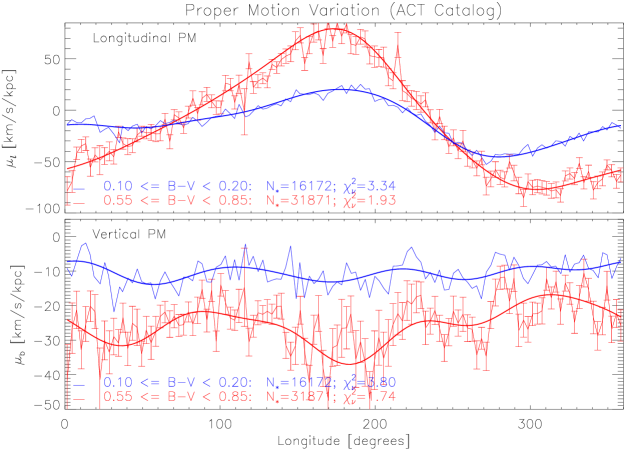
Figure 2: The longitudinal variation for a group of “red” and “blue” stars. We plot ${\overline{\mu}}_{\ell^{\star}}$ and $\mu_{b}$ in the top and bottom panels, respectively. The jagged lines with and without error bars represent the red and blue main-sequence stars, respectively. We also plot the Fourier fits as the thick smooth lines, and list the number of stars used, as well as the reduced $\chi^{2}$ values. The curves with the larger amplitudes correspond to the red stars. Only stars with $|\sin(b)|\leq 0.1$ are included.

One may show that the longitudinal dependence of the mean parallax induced just by a smooth exponential stellar disk is small. However, as we will see below, the stars are very non-uniformly distributed in $\ell$. This is a clear indication of inhomogeneity in the spatial distribution of the sample stars. This inhomogeneity is caused both by an intrinsic clumpiness of the stellar density and by extinction blocking the view through the Galaxy in a highly inhomogeneous and anisotropic way. Thus, we expect ${\overline{\pi}}$ to be non-uniform as well, causing considerable mode mixing.

In Figure 2 we present graphically the longitudinal variation of ${\overline{\mu}}_{\ell^{\star}}$ and $\mu_{b}$ for two groups of stars with different colors. The “jagged” lines represents the data, the smooth lines the Fourier fits. We clearly see that the vertical proper motion exhibits azimuthal variation of about $\pm$ 35% (bottom panel), indicating a changing average parallax with longitude. The reduced $\chi^{2}$ values listed are computed with respect to a 5^th order Fourier-fit model and indicate that the fits are “reasonable.” However, because the distribution of the proper motions in each longitude bin of 3^o is not quite normal, the $\chi_{\nu}^{2}$ values are only indicative of the goodness of fit. Assuming a simpler model with constant $\mu_{b}(\ell)$ lead to 60% larger $\chi_{\nu}^{2}$ values, proving that the observed variation is real. The mean levels of the vertical proper motion indicate that the red stars are about three times closer than the blue stars.

2.7.2 A Cure from the Effect?

In order to correct for this effect, one needs some unbiased estimate of the relative Fourier coefficients $(c_{\pi},s_{\pi})_{m}$ for the mean stellar parallax, defined in equation (14).

Fortunately, for $b=0$ equation (15b) simplifies considerably to

$${\overline{\mu}}_{b}|_{b=0}=-{\overline{\mu}}_{W0}\Big{(}1+2\sum_{m}c_{\pi m}\cos m\ell+s_{\pi m}\sin m\ell\Big{)}.$$ (18)

Thus, for low latitudes we can use the vertical stellar proper motions to measure, apart from ${\overline{\mu}}_{W0}$, the relative Fourier coefficients $(c_{\pi},s_{\pi})_{m}$ of ${\overline{\pi}}$ and use them to correct the Fourier coefficients obtained from ${\overline{\mu}}_{\ell^{\star}}$ (see §3.2 for details of our measurement technique). However, this works only, if the vertical solar reflex motion $W_{0}$, or equivalently, the mean vertical motion of the stars with respect to the Sun is constant with $\ell$. A stellar warp, for example, would invalidate this assumption. Fortunately, it seems from Dehnen’s (1998) analysis of the local stellar velocity distribution that the stellar warp only weakly affects our analysis: only stars at $R-R_{0}\gtrsim 1\,\mbox{${\rm kpc}$}$ or with high $V$-velocity are affected.

If this assumption of constant $W_{0}$ is doubtful, or if high-latitude stars are concerned, the only possible cure of the problem is an unbiased, but not necessarily very accurate, distance measure, which can be used to independently estimate the Fourier coefficients of ${\overline{\pi}}$. Using the photometric parallaxes for this purpose does not work – we tried it – presumably since extinction affects the distributions of true and photometric parallax in fundamentally different ways, but perhaps also because of systematic errors in the photometric parallax (cf. Malmquist bias).

2.7.3 Mode Mixing and Distance Effects

In §2.4 we have seen that for a conventional parameterizations of the average Galactic streaming field, distance effects result in $\cos{\ell}$ and $\cos{3\ell}$ amplitudes of order of several ${\rm km}\,{\rm s}^{-1}\,{\rm kpc}^{-1}$. Such contributions are comparable to those expected from mode-mixing effects (§2.7.1). Thus, for samples that are sufficiently deep for these distance effects to be important one cannot disentangle the two contributions, and a correction of the mode mixing from proper motion data alone becomes impossible. We will return to this point in the discussion of the results obtained from proper-motion data.

2.8 Measurement Accuracy

2.8.1 Internal Uncertainties

It is instructive to estimate the expected uncertainty for $\tilde{A}$, $\tilde{B}$, and $\tilde{C}$ determined from the proper motions of a large stellar sample ($\tilde{K}$ can only be sensibly measured from radial velocities). The observed proper motion for an individual star can be described by the mean plus a random component and an error term. The mean as function of $(\ell,b)$ is given by equation (11) (neglecting mode mixing). The random component has two sources: random stellar motions leading to a random component proportional to parallax, and scatter in stellar parallaxes resulting in scatter in the terms arising from the solar reflex motion.

For a stellar sample uniformly distributed inside a radius $d_{\rm max}$, with mean motion with respect to the Sun of 20 ${\rm km}\,{\rm s}^{-1}$, and a one-dimensional velocity dispersion in the plane of 30 ${\rm km}\,{\rm s}^{-1}$, the dispersion of the random proper motion amounts to roughly $50/d_{\rm max}\,\mbox{${\rm km}\,{\rm s}^{-1}\,{\rm kpc}^{-1}$}$. Thus, in order to measure the Oort constants to an accuracy of $\epsilon$, we need of the order of $N=2500\times d_{\rm max}^{-2}\times(\epsilon/\mbox{${\rm km}\,{\rm s}^{-1}\,{\rm kpc}^{-1}$})^{-2}$ stars. If one increases the accuracy by using ever deeper samples, one must be aware that, as discussed in §2.5 above, the measurable Oort constants are functions of sample depth. From this estimate, it is clear that the measurement uncertainties in the observed proper motions are almost always negligible in the error budget.

2.8.2 Systematic Errors

There is, however, another well known source of uncertainty: a residual systematic rotation of the astrometric reference system used to measure the individual proper motions. The rotation frequency simulates a vorticity of the velocity field, and its $z$ component is indistinguishable from $\tilde{B}$. For ground-based proper-motion surveys, one can only with great difficulty establish an inertial reference frame, and in many cases some residual rotation remains (see Kovalevsky et al., 1997, for a recent review). For example, the rotation of the Hipparcos reference frame is estimated to be no larger than 0.25 mas yr${}^{-1}=1.18\,\mbox{${\rm km}\,{\rm s}^{-1}\,{\rm kpc}^{-1}$}$ (Kovalevsky et al., 1997). This implies that $B$ cannot be accurately measured, even when using the best astrometric reference system currently available!

3 The Measurement Technique

The classical way used to determine the Oort constants from proper motions ${\boldsymbol{\mu}}\equiv({\overline{\mu}}_{\ell^{\star}},\mu_{b})$ is a least-squares fit of equation (11) to the observed proper motions. Hanson (1987), for instance, employed this method to determine just $A$ and $B$ from the NPM survey. This straightforward approach, however, cannot be recommended. The main problem is that the actual functional form of the mean proper motion ${\overline{{\boldsymbol{\mu}}}}(\ell,b)$ is possibly not well described by the fitting function (see §2). As with all parametric methods, such a mismatch inevitably leads to systematic errors in the values obtained for the parameters.

As already discussed in §2.1 and §2.3 above, the measurable Oort constants and the relative mean proper motions ${\overline{\mu_{U}}},\,{\overline{\mu_{V}}},\,{\overline{\mu_{W}}}$ are functions of stellar type and latitude. These variations introduce an a priori unknown dependence of ${\overline{{\boldsymbol{\mu}}}}$ on latitude $b$. In his analysis Hanson accounted for a variation of ${\overline{{\boldsymbol{\mu}}}}_{\odot}$, but did not find a latitude dependence of $A$ and $B$. Additional to the expected variations with latitude, there will be variations of ${\overline{{\boldsymbol{\mu}}}}$ with longitude as discussed in §2.4 and §2.5. The stars are always non-uniformly distributed in $\ell$ such that the harmonics e^imℓ are not orthogonal under averaging over $\ell$. This implies that, if there is (non-anticipated) power in higher-order harmonics, fitting only the low-order ($m\leq 2$) harmonics again introduces systematic errors in the parameter values obtained.

In order to avoid these problems, we expand ${\overline{{\boldsymbol{\mu}}}}$ in a Fourier series including high orders and restrict ourselves to a small range of latitudes. This is an essentially non-parametric approach in that it allows for a general functional form for ${\overline{{\boldsymbol{\mu}}}}(\ell)$ and avoids variations at high latitudes. To be more specific we determine the coefficients $c_{\ell m}$, $s_{\ell m}$, $c_{bm}$, and $s_{bm}$ of

$${\overline{\mu}}_{\ell^{\star}} = c_{\ell 0}+\sum_{m>0}^{m_{\rm max}}c_{\ell m}\cos m\ell+s_{\ell m}\sin m\ell,$$ (19a)

$${\overline{\mu}}_{b} = c_{b0}+\sum_{m>0}^{m_{\rm max}}c_{bm}\cos m\ell+s_{bm}\sin m\ell$$ (19b)

by a least-squares fit to the observed ${\overline{\mu}}_{\ell^{\star}}$ and $\mu_{b}$ (see also §3.3.1 below).

3.1 Weighting and Exclusion of Outliers

In order to minimize the errors, one might weight individual stars with the inverse variance of their proper motion. This is essentially given by the stars parallax times the velocity dispersion, see §2.8 above. The latter is a function of color, and, since we will analyze the stars in color bins, the weights reduce to $10^{-0.4m}$ where $m$ is the apparent magnitude in some passband. Such a technique greatly increases the importance of the faintest and most distant stars in the sample, i.e. those objects that are most likely affected by extinction. Experimenting with such a scheme, we found no significant reduction in the estimated uncertainties.

Another method to reduce the errors is to exclude high-proper-motion stars. For example, $\kappa$-$\sigma$-clipping excludes stars whose ${\overline{\mu}}_{\ell^{\star}}$ or $\mu_{b}$ deviates from the mean at their longitude by more than $\kappa$ times the dispersion $\sigma$. This approach is somewhat dangerous as it uses kinematic information itself in a study aimed at kinematic quantities.

The most conservative technique is to exclude just bright stars, since these are most likely very near and their proper motions are dominated by random velocities.

3.2 Correction for Mode Mixing

Having obtained the raw Fourier coefficients $(c_{\ell},s_{\ell},c_{b},s_{b})_{m}$, we might want to correct them for the mode mixing described in §2.7, i.e. extract the Fourier coefficients that would have been measured without longitudinal variations in the mean parallax. Equating (19) to (15) one gets a linear relation between the raw Fourier coefficients $(c_{\ell},s_{\ell},c_{b},s_{b})_{m}$ and the unknowns

$${\boldsymbol{\xi}}\equiv({\overline{\mu}}_{U0},\,{\overline{\mu}}_{V0},\,{\overline{\mu}}_{W0},\,\tilde{A},\,\tilde{B},\,\tilde{C},\,\ldots),$$ (20)

where the dots stands for possible higher-order terms.

3.2.1 At Low Latitudes

As pointed out in §2.7, at low latitudes ${\overline{\sin b}}\simeq 0$, i.e. the Galactic-rotation induced higher-order terms in ${\overline{\mu}}_{b}$ vanish, and we can use ${\overline{\mu}}_{b}$ to directly measure the mode-mixing coefficients ${\boldsymbol{\alpha}}\equiv(c_{\pi},s_{\pi})_{m}$, see Equations (14) and (18). In §4 below, we will determine the unknowns ${\boldsymbol{\xi}}$ up to order $m=4$, and need the mode-mixing coefficients and hence the raw Fourier coefficients of ${\overline{\mu}}_{b}$ up to order $m=5$. Thus, we have 20 (non-linear) equations (9 from ${\overline{\mu}}_{\ell^{\star}}$ and 11 from ${\overline{\mu}}_{b}$) for 20 unknowns (10 from ${\boldsymbol{\xi}}$ and 10 from ${\boldsymbol{\alpha}}$).

3.2.2 At High Latitudes

At high latitudes, we cannot estimate ${\boldsymbol{\alpha}}$ directly from the proper motions. However, if one is only interested in the low-order coefficients (up to $m=2$ in equation (15), the situation is not too bad, as there are 10 equations for 6 unknowns in ${\boldsymbol{\xi}}$ and another 6 in ${\boldsymbol{\alpha}}$. Thus, even though the equations have no unique solution, there is no complete freedom in the possible mode mixing. In order to get a unique answer, one may postulate that mode mixing is minimal, i.e. seek the smallest ${\boldsymbol{\alpha}}$ that solves the equations.

Note that in the analysis presented in §4 we will restrict ourselves to low latitudes and use the procedure outlined in §3.2.1.

3.3 Numerics and Error Analysis

3.3.1 The Raw Fourier Coefficients

Let us, for convenience, denote the vector of Fourier coefficients $(c,s)_{m}$ by ${\boldsymbol{c}}$ and that of the harmonic basis functions by ${\boldsymbol{y}}$. Then, we determine ${\boldsymbol{c}}$ by minimizing the sample average $\left\langle{(\mu-{\boldsymbol{c}}\cdot{\boldsymbol{y}})^{2}}\right\rangle$ giving

$${\boldsymbol{c}}=\left\langle{{\boldsymbol{y}}\otimes{\boldsymbol{y}}}\right\rangle^{-1}\cdot\left\langle{\mu{\boldsymbol{y}}}\right\rangle.$$ (21)

The variance ${\bf V}_{{\boldsymbol{c}}}$ is computed via error-propagation from the variance of $\langle{\mu{\boldsymbol{y}}}\rangle$, which is given by the standard formula

$$\mathbf{V}_{\langle{\mu{\boldsymbol{y}}}\rangle}=\frac{\left\langle{\mu{\boldsymbol{y}}\otimes\mu{\boldsymbol{y}}}\right\rangle-\left\langle{\mu{\boldsymbol{y}}}\right\rangle\otimes\left\langle{\mu{\boldsymbol{y}}}\right\rangle}{N-1}.$$ (22)

3.3.2 Correction for Mode Mixing

The ${\boldsymbol{c}}_{i}$, $i=\ell,b$, are linearly related to our desired quantity ${\boldsymbol{\xi}}$,

$${\boldsymbol{c}}_{i}={\bf M}_{i}\cdot{\boldsymbol{\xi}},$$ (23)

where the matrices ${\bf M}_{i}$ are given through equation (15) and depend linearly on the mode-mixing coefficients ${\boldsymbol{\alpha}}$. Let

$$\chi^{2}_{{\boldsymbol{\mu}}}=\sum_{i=\ell,b}({\boldsymbol{c}}_{i}-\mathbf{M}_{i}\cdot{\boldsymbol{\xi}})^{T}\,\mathbf{V}_{{\boldsymbol{c}}_{i}}^{-1}\,({\boldsymbol{c}}_{i}-\mathbf{M}_{i}\cdot{\boldsymbol{\xi}})$$ (24)

be the error-weighted deviation from this relation. Solving (23) is equivalent to minimizing (24) with respect to ${\boldsymbol{\xi}}$ and ${\boldsymbol{\alpha}}$. The variance ${\bf V}_{{\boldsymbol{\xi}}}$ is then given by the ${\boldsymbol{\xi}}$-part of twice the inverse of the Hessian matrix of $\chi^{2}_{{\boldsymbol{\mu}}}$.

4 Analysis of the Proper Motion Catalogs

The coordinate system defined by the Hipparcos Catalogue (ESA, 1997) is currently the best realization of an inertial reference frame (Kovalevsky et al., 1997). It is thus expedient to re-determine the Oort constants using proper motion data based on this reference frame. Unfortunately, the Hipparcos Catalogue itself is not a kinematically unbiased catalog, so that special care has to be taken when inferring kinematic properties from it (Binney et al., 1997). A kinematically unbiased subsample extracted from the Hipparcos Catalogue by DB98 contains about 14 000 stars with a maximum and average distance of about 100 and 80 parsec. Using our estimate from §2.8 for the accuracy of the Oort constants, we expect for this sample an uncertainty of the Oort constants of about 4 ${\rm km}\,{\rm s}^{-1}\,{\rm kpc}^{-1}$, which is unacceptably large.

In order to get more accurate estimates for the Oort constants, one needs deeper and/or larger samples. In the present paper we will employ the ACT Catalog (Urban, Corbin & Wycoff, 1998), which is essentially magnitude limited, and hence kinematically unbiased. The ACT Catalog is a combination of the Astrographic Catalog (Eichhorn, 1974; Corbin & Urban, 1988; Urban et al., 1998) with a median epoch near 1904, and the Tycho Catalogue (ESA, 1997), which has a limiting magnitude of about $V=11.5$. It contains, for nearly $10^{6}$ stars, two color photometry and accurate astrometric data (positions and proper motions) defined in the Hipparcos reference frame.

We have also analyzed the Tycho-2 catalog (Hog et al., 2000a). This catalog entails a re-analysis of the data of Hipparcos’ Tycho instrument, the astrographic catalog and many other astrometric datasets (Hog et al., 2000b). This catalog contains about twice as many stars as ACT catalog, where the majority of the “extra” stars are fainter than $V_{T}\sim 10$, while its astrometry is equivalent to that of the ACT catalog (Hog et al., 2000a). It might be tempting to use the larger Tycho-2 catalog instead of the ACT. However, a twice larger sample means a roughly 40% larger limiting distance, so that the distance-dependent effects and higher-order terms may become important (see §2.4). Instead we decided to use the ACT catalog, and verify the results by a similar analysis of the Tycho-2 data over the ACT magnitude range ($8.5\leq V_{T}\leq 11.5$). Since the ACT and Tycho-2 results are entirely consistent with each other, we will use the term “ACT/Tycho-2” to describe our data in the remainder of this paper.

Compared to the Hipparcos sub-sample, the sample-depth and the number of stars is increased by factors of about ten and 70, respectively. Estimating the expected accuracy for the Oort constants, one realizes that we may even divide this sample into subsets and still get reasonably accurate values for $\tilde{A}$, $\tilde{B}$, and $\tilde{C}$.

Figure 3: The distributions $n(\ell)$ (in arbitrary units) of the stars in the color bins 1 to 10, see Table 4.1 for the limits in $\bv$.

4.1 Longitudinal Inhomogeneities

As discussed in §2.3, spatial inhomogeneity and extinction are expected to bias the Oort constants and to confuse them via mode mixing. We are able, though, to correct for the latter effect provided we restrict ourselves to low latitudes. For this reason, since the stellar density is highest there, and because we are mainly interested in the Oort constants in the Galactic plane, we restrict our analysis to stars with $|\sin b|\leq 0.1$ ($|b|\lesssim 5.74^{\circ}$). After further excluding stars brighter than $m_{B}=8.5$ (§3.1), we are left with 192 546 stars in the color range $\bv\in[-0.2,4]$.

Table 1
The Color Bins

#		$\bv$		$N$	$\delta n(\ell)$	$\frac{1}{{\overline{\pi_{W}}}}$	$(\bv)_{0}$	$\tau_{\mathrm{MS}}$	$f_{Y}$
1		–0.20 -	0.00	7,843	0.272	0.652	–0.31	0.01	100
1	a	–0.10 -	0.05	12,931	0.236	0.732	–0.26	0.02	100
2		0.00 -	0.10	14,345	0.180	0.724	–0.18	0.03	100
2	a	0.05 -	0.15	16,490	0.139	0.703	–0.13	0.07	100
3		0.10 -	0.20	17,708	0.120	0.683	–0.07	0.18	100
3	a	0.15 -	0.25	18,890	0.111	0.646	–0.01	0.38	100
4		0.20 -	0.30	19,097	0.095	0.583	0.06	0.59	100
4	a	0.25 -	0.36	21,211	0.088	0.539	0.13	0.77	100
5		0.30 -	0.42	23,611	0.085	0.488	0.20	1.07	100
5	a	0.36 -	0.50	27,824	0.071	0.422	0.29	1.64	91
6		0.42 -	0.55	25,815	0.059	0.375	0.36	2.61	57
6	a	0.50 -	0.70	30,619	0.041	0.301	0.50	5.55	27
7		0.55 -	0.85	31,234	0.043	0.279	0.61	8.41	18
7	a	0.70 -	0.97	17,987	0.089	0.309	0.74	$\cdots$	64
8		0.85 -	1.10	18,056	0.137	0.475	0.82	$\cdots$	100
8	a	0.97 -	1.20	17,993	0.122	0.578	0.90	$\cdots$	96
9		1.10 -	1.35	16,072	0.083	0.652	1.01	$\cdots$	58
9	a	1.20 -	1.50	14,198	0.065	0.747	1.11	$\cdots$	40
10		1.35 -	1.90	12,797	0.046	0.854	1.35	$\cdots$	22

Note.— The boundaries of the (observed) B V color; number $N$ of stars fainter than $V_{T}=8.5$; relative overabundance in $n(\ell)$ (see §4.1); Average inverse parallax [in kpc, see equation (26b)]; our best estimate of the intrinsic color; the main-sequence lifetime $\tau_{\mathrm{MS}}$ (in Gyr; bins 7a–10 comprise non-MS stars); and the percentage $f_{Y}$ of stars younger than 1.5 Gyr. For the main-sequence stars, we estimate $f_{Y}$ from the MS lifetime and a constant SFR, for the post-MS star, we employ the $\delta n(\ell)$ method, see §5.1.1 for details.

In order to get a feeling for the importance of the spatial inhomogeneities, we binned the stars into 60 bins in $\bv$ and considered their longitudinal frequency, $n(\ell)$. Figure 3 plots $n(\ell)$ for the color bins 1 to 10 (see Table 4.1) used in the analysis below. Most prominent in the bluest color bin (#1) are three peaks near $\ell\simeq 75^{\circ},\,240^{\circ}$, and $285^{\circ}$, which presumably are caused by stars in the Sagittarius-Carina ($\ell=75\arcdeg$, $285\arcdeg$) and the Orion-Cygnus ($\ell=240\arcdeg$) spiral-arms. In order to quantify how important these peaks are, we measured the relative number $\delta n(\ell)$ of stars in three windows of $30^{\circ}$ width that were centered on the three peaks, and subtracted $1/4$, the expectation value for a uniform distribution. Figure 4 plots this measure versus the mean color for 60 narrow color bins (open), as well as the 19 bins used in the analysis below (solid). The importance of the peaks is largest at the blue end, where the stars are very young and not mixed or settled into equilibrium. Moreover, these stars are very bright and can be seen out to a few ${\rm kpc}$, such that patchy extinction can best contribute to the apparent non-uniformity. Along the main sequence (MS), where the stars get older, hence better mixed, and fainter, $n(\ell)$ steadily becomes more uniform until $\bv\simeq 0.7$. Then the peaks become important again near $\bv\approx 1$, where the red clump dominates the sample, while the giants at $\bv\gtrsim 1.2$ are nearly as uniformly distributed as are the dwarfs near $\bv\simeq 0.7$.

The red-most of the 60 narrow bins at $\bv=1.95$ is somewhat odd, as it has less stars in those peaks than even for uniform $n(\ell)$. The likely reason is that these are stars subject to severe extinction, which made them appear much redder than they really are (there are no stars with intrinsic $\bv>2$), and restricts them to regions where high extinction has diminished the numbers in the other color bins.

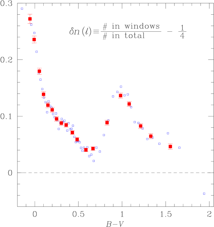
Figure 4: The relative over-abundance of stars, $\delta n(\ell)$, in three $30^{\circ}$ wide windows centered on the peaks that dominate $n(\ell)$ for the bluest stars. The open symbols are for 60 color bins while the solid squares represent the 19 bins used in the analysis; see also LABEL:nl for $n(\ell)$ of these ten bins.

4.2 Data Analysis

4.2.1 Binning and Analyzing the Data

Before the analysis in terms of the Oort constants, we split the data it into ten color bins, labeled 1 to 10. These bins have been chosen to group together stars with similar $n(\ell)$. Small bins had to be avoided, in particular at red colors, to yield reasonable errors for the Oort constants – large errors would render differences between the results of adjacent bins insignificant. In addition to these ten distinct bins, we consider 9 bins of similar size (labeled 1a to 9a) whose stars are taken half from each of the nearest primary bins. The color limits of all the 19 bins are given in Table 4.1, which also lists the numbers of stars fainter than $V_{T}=8.5$ contained in each bin.

To reduce the errors, we also analyzed the data after applying a modest $\kappa$-$\sigma$-clipping with $\kappa=5$ and excluding not more than 5% of the stars in each of 20 longitudinal bins (the only usage ever of such bins). The raw Fourier coefficients for ${\overline{\mu}}_{\ell^{\star}}$ and ${\overline{\mu}}_{b}$ and their errors were estimated up to $m_{\rm max}=32$ as outlined in §3.3.1 and are tabulated up to $m=5$ in Tables 4.2.1 and 4.2.1 for all 19 color bins. Note that if there were no mode mixing, $\tilde{A}$, $\tilde{B}$, and $\tilde{C}$ could be read of Table 4.2.1 as $c_{2}$, $c_{0}$, and $-s_{2}$.

Table 2: Raw Fourier Coefficients for ${\overline{\mu}}_{\ell^{\star}}$

bin		$c_{0}$		$c_{1}$		$s_{1}$		$c_{2}$		$s_{2}$		$c_{3}$		$s_{3}$		$c_{4}$		$s_{4}$		$c_{5}$		$s_{5}$
1		–11.8${\pm}$	1.1	–13.9${\pm}$	1.7	9.8${\pm}$	1.5	12.4${\pm}$	1.5	–0.2${\pm}$	1.7	–0.1${\pm}$	1.4	–5.4${\pm}$	1.8	0.7${\pm}$	1.7	0.0${\pm}$	1.6	–0.1${\pm}$	1.7	1.4${\pm}$	1.6
1	a	–12.0${\pm}$	0.6	–14.6${\pm}$	1.0	12.1${\pm}$	0.8	11.8${\pm}$	0.8	1.1${\pm}$	0.9	0.4${\pm}$	0.7	–4.8${\pm}$	1.0	0.4${\pm}$	0.9	1.4${\pm}$	0.9	0.1${\pm}$	0.9	1.3${\pm}$	0.9
2		–11.9${\pm}$	0.4	–15.4${\pm}$	0.6	13.3${\pm}$	0.5	13.4${\pm}$	0.5	1.7${\pm}$	0.6	0.9${\pm}$	0.4	–4.4${\pm}$	0.7	0.1${\pm}$	0.5	1.2${\pm}$	0.6	–0.7${\pm}$	0.5	0.8${\pm}$	0.6
2	a	–11.9${\pm}$	0.3	–17.2${\pm}$	0.5	14.0${\pm}$	0.4	14.2${\pm}$	0.4	1.8${\pm}$	0.5	0.7${\pm}$	0.4	–3.4${\pm}$	0.5	–0.1${\pm}$	0.5	0.5${\pm}$	0.5	0.0${\pm}$	0.5	0.4${\pm}$	0.5
3		–11.9${\pm}$	0.4	–17.9${\pm}$	0.6	14.0${\pm}$	0.5	14.7${\pm}$	0.5	1.8${\pm}$	0.6	–0.0${\pm}$	0.5	–3.9${\pm}$	0.7	0.2${\pm}$	0.5	0.8${\pm}$	0.7	0.6${\pm}$	0.6	–0.0${\pm}$	0.6
3	a	–11.8${\pm}$	0.4	–19.3${\pm}$	0.6	14.3${\pm}$	0.5	15.6${\pm}$	0.5	1.3${\pm}$	0.6	–1.0${\pm}$	0.5	–3.6${\pm}$	0.6	0.8${\pm}$	0.6	0.1${\pm}$	0.6	1.0${\pm}$	0.6	0.6${\pm}$	0.5
4		–12.0${\pm}$	0.4	–21.9${\pm}$	0.6	15.8${\pm}$	0.6	14.8${\pm}$	0.6	0.9${\pm}$	0.6	–0.7${\pm}$	0.6	–3.2${\pm}$	0.6	0.6${\pm}$	0.6	–0.5${\pm}$	0.6	1.2${\pm}$	0.7	0.8${\pm}$	0.6
4	a	–12.1${\pm}$	0.5	–25.6${\pm}$	0.8	17.4${\pm}$	0.6	14.7${\pm}$	0.7	1.4${\pm}$	0.7	–0.4${\pm}$	0.7	–3.3${\pm}$	0.7	0.9${\pm}$	0.6	–0.0${\pm}$	0.8	0.6${\pm}$	0.7	–0.2${\pm}$	0.7
5		–12.4${\pm}$	0.6	–28.8${\pm}$	0.9	20.3${\pm}$	0.7	15.7${\pm}$	0.8	1.6${\pm}$	0.8	–1.6${\pm}$	0.8	–3.2${\pm}$	0.9	1.5${\pm}$	0.8	0.1${\pm}$	0.8	0.4${\pm}$	0.9	–0.8${\pm}$	0.8
5	a	–11.7${\pm}$	0.6	–36.2${\pm}$	0.9	24.5${\pm}$	0.7	18.2${\pm}$	0.9	1.6${\pm}$	0.8	–1.9${\pm}$	0.8	–3.4${\pm}$	0.8	–0.3${\pm}$	0.8	–0.4${\pm}$	0.8	–0.8${\pm}$	0.9	–1.0${\pm}$	0.8
6		–10.7${\pm}$	0.7	–43.9${\pm}$	1.0	26.5${\pm}$	0.9	18.8${\pm}$	1.0	2.0${\pm}$	0.9	–1.9${\pm}$	1.0	–2.8${\pm}$	1.0	–0.1${\pm}$	1.0	0.5${\pm}$	0.9	–1.7${\pm}$	1.0	–0.6${\pm}$	0.9
6	a	–9.6${\pm}$	0.9	–63.7${\pm}$	1.3	30.9${\pm}$	1.1	17.7${\pm}$	1.3	3.0${\pm}$	1.2	–3.7${\pm}$	1.2	–1.8${\pm}$	1.3	1.7${\pm}$	1.2	0.5${\pm}$	1.3	–0.4${\pm}$	1.3	0.8${\pm}$	1.3
7		–9.6${\pm}$	1.0	–75.7${\pm}$	1.5	32.1${\pm}$	1.3	16.4${\pm}$	1.5	1.9${\pm}$	1.4	–5.2${\pm}$	1.4	–2.4${\pm}$	1.4	1.3${\pm}$	1.4	–1.1${\pm}$	1.5	–0.5${\pm}$	1.4	0.9${\pm}$	1.4
7	a	–9.8${\pm}$	1.4	–81.1${\pm}$	2.2	28.9${\pm}$	1.7	11.6${\pm}$	2.2	–5.7${\pm}$	1.9	–7.7${\pm}$	2.1	0.8${\pm}$	2.0	0.5${\pm}$	2.1	–3.5${\pm}$	2.0	–2.1${\pm}$	2.0	–0.1${\pm}$	2.1
8		–9.8${\pm}$	1.4	–60.2${\pm}$	2.2	23.5${\pm}$	1.7	13.7${\pm}$	1.9	–9.4${\pm}$	2.1	–2.6${\pm}$	1.8	4.7${\pm}$	2.2	–0.8${\pm}$	2.0	–5.3${\pm}$	2.0	1.8${\pm}$	2.0	1.9${\pm}$	2.0
8	a	–12.2${\pm}$	1.1	–45.9${\pm}$	1.8	20.1${\pm}$	1.4	14.2${\pm}$	1.5	–5.4${\pm}$	1.8	0.2${\pm}$	1.4	1.3${\pm}$	1.9	0.1${\pm}$	1.6	–3.8${\pm}$	1.7	3.7${\pm}$	1.6	2.1${\pm}$	1.8
9		–13.6${\pm}$	1.0	–40.0${\pm}$	1.6	15.3${\pm}$	1.4	13.7${\pm}$	1.3	–0.5${\pm}$	1.7	–0.8${\pm}$	1.3	–0.6${\pm}$	1.7	1.6${\pm}$	1.6	–0.8${\pm}$	1.4	0.7${\pm}$	1.6	0.4${\pm}$	1.4
9	a	–12.8${\pm}$	1.1	–38.6${\pm}$	1.7	13.9${\pm}$	1.5	14.2${\pm}$	1.3	–1.9${\pm}$	1.9	0.0${\pm}$	1.5	1.5${\pm}$	1.8	1.0${\pm}$	1.8	–2.0${\pm}$	1.4	0.5${\pm}$	1.9	1.1${\pm}$	1.4
10		–12.2${\pm}$	0.9	–30.5${\pm}$	1.3	13.5${\pm}$	1.2	13.8${\pm}$	1.0	–3.0${\pm}$	1.5	1.2${\pm}$	1.2	1.7${\pm}$	1.4	–0.9${\pm}$	1.4	–1.4${\pm}$	1.3	0.4${\pm}$	1.3	1.7${\pm}$	1.3

with $\kappa$-$\sigma$-clipping    1 –13.30.6 –15.30.9 11.80.9 13.10.7 0.51.0 0.30.8 –4.81.0 2.30.9 0.71.0 1.31.0 2.20.8 1a –12.50.4 –15.20.6 13.00.6 13.20.5 1.50.7 0.40.5 –4.20.7 1.00.6 1.00.6 0.10.6 1.80.5 2 –11.90.3 –15.80.4 13.60.4 13.50.4 1.70.5 1.20.4 –3.90.5 0.10.5 1.10.4 –0.10.5 0.90.4 2a –11.90.2 –17.00.4 13.80.4 13.70.3 1.70.4 1.10.3 –3.40.4 0.20.4 0.90.4 0.30.4 0.60.4 3 –12.00.2 –18.20.4 13.80.3 14.50.3 1.50.4 0.20.3 –3.40.4 0.30.4 0.20.4 0.60.4 0.60.4 3a –11.90.2 –19.50.3 14.10.3 14.80.4 1.70.4 –0.80.3 –3.10.4 0.20.4 –0.30.4 0.40.4 0.90.4 4 –11.80.3 –20.90.4 16.10.4 14.60.4 2.40.4 –1.10.4 –2.50.4 0.10.4 –0.30.4 0.00.4 0.90.4 4a –11.50.3 –23.10.4 18.10.4 15.40.4 2.50.4 –0.50.4 –2.70.4 1.00.4 0.00.4 –0.20.4 0.30.4 5 –11.00.3 –25.60.5 20.30.4 16.20.5 2.70.5 –1.00.4 –2.70.5 0.80.5 –0.10.5 –0.10.5 0.10.5 5a –10.90.4 –31.90.5 23.70.5 18.00.6 3.00.5 –1.70.5 –2.50.6 0.20.5 –0.10.6 –0.50.6 –0.10.5 6 –10.70.5 –38.70.7 25.10.7 18.60.7 2.60.7 –1.90.7 –2.10.7 0.40.7 1.40.7 –0.60.7 –0.80.7 6a –9.90.6 –53.80.9 28.30.9 17.61.0 3.20.9 –3.70.9 –2.20.9 1.30.9 0.60.9 –1.60.9 –0.00.9 7 –9.60.7 –63.51.0 30.41.0 18.11.1 1.51.0 –3.51.0 –1.31.0 1.71.0 –0.81.1 –0.81.0 –0.51.0 7a –10.11.0 –66.21.5 27.11.3 13.21.5 –7.41.5 –3.91.4 1.71.5 0.51.4 –4.31.5 0.21.4 –2.31.5 8 –9.50.7 –42.21.2 19.70.9 15.71.0 –5.61.2 –0.31.0 3.81.2 –2.21.1 –3.81.1 2.61.1 1.11.0 8a –11.30.5 –34.20.8 16.30.7 16.40.7 –0.20.8 0.20.7 1.20.9 –0.10.8 –1.10.8 1.30.8 0.80.8 9 –12.70.5 –33.00.7 14.30.6 15.40.7 2.00.7 –0.50.7 0.60.7 0.90.7 0.40.7 –0.10.7 0.60.7 9a –12.60.4 –31.60.6 13.90.6 14.40.7 1.00.7 –0.00.6 1.40.7 0.30.7 0.10.7 –0.90.7 1.20.7 10 –12.50.4 –27.40.6 13.00.6 14.20.6 –1.00.6 0.90.6 2.10.6 –1.20.6 0.30.6 –0.90.6 1.40.6

Table 3: Raw Fourier Coefficients for ${\overline{\mu}}_{b}$

1 –11.01.6 –0.92.6 –0.91.8 –1.11.1 –3.22.8 2.80.9 –3.72.9 1.32.2 0.02.1 2.22.8 0.20.8 1a –9.80.3 1.00.6 0.40.4 0.00.3 –0.50.6 1.90.3 –1.00.6 –0.10.5 1.40.5 0.00.6 0.30.4 2 –9.90.2 1.30.3 0.10.3 0.30.2 –0.30.4 1.60.2 –0.40.4 0.20.3 1.10.3 0.30.3 0.40.3 2a –10.20.1 1.20.3 –0.00.2 0.40.2 –0.30.3 1.30.2 –0.40.3 0.30.2 1.10.2 0.50.3 0.60.2 3 –10.50.1 1.00.3 –0.40.2 0.40.2 –0.80.2 1.30.2 –0.70.3 –0.00.2 1.30.2 0.50.2 0.50.2 3a –11.10.1 1.60.3 –0.70.2 –0.10.2 –0.90.2 1.30.2 –1.00.2 –0.20.2 1.20.2 0.20.2 0.50.2 4 –12.30.1 1.70.3 –0.30.2 –0.40.2 –1.20.2 1.50.2 –1.20.3 –0.10.2 1.20.2 –0.20.3 0.50.2 4a –13.30.1 2.10.3 –0.20.2 –0.50.2 –1.60.2 2.10.2 –1.20.3 –0.10.2 1.40.2 0.10.2 0.80.2 5 –14.70.2 2.80.3 –0.90.2 –0.70.3 –1.80.3 2.00.3 –1.20.3 –0.10.3 1.30.3 0.60.3 0.80.3 5a –17.00.2 3.70.3 –0.40.3 –0.60.3 –2.00.3 1.70.3 –1.30.3 –0.40.3 0.80.3 0.70.3 0.60.3 6 –19.10.2 3.70.5 –0.20.3 –1.20.4 –2.60.4 1.40.4 –1.00.4 –0.30.4 0.60.4 1.00.4 0.60.4 6a –23.80.3 2.90.6 –1.10.5 –2.50.5 –3.00.5 0.50.5 –2.10.5 –0.20.5 –0.40.5 0.50.5 0.40.5 7 –25.70.4 3.80.7 –1.70.5 –3.50.6 –3.50.6 1.60.6 –2.50.6 –1.10.6 –0.70.6 1.20.6 0.80.6 7a –23.20.6 1.81.0 –4.70.7 –5.20.9 –2.90.8 0.90.8 –3.60.9 –1.40.8 –0.90.9 2.50.8 0.70.9 8 –15.10.4 0.80.7 –3.80.5 –2.80.6 –1.70.7 –1.20.6 –3.20.7 0.20.6 0.00.7 1.20.7 0.40.6 8a –12.40.3 1.70.5 –2.10.4 –2.00.4 –1.20.5 –0.10.4 –2.20.5 –0.60.5 0.10.5 0.60.5 –0.30.4 9 –11.00.2 1.70.4 –2.40.3 –1.60.4 –1.30.4 0.20.4 –1.90.4 –0.80.4 0.30.4 1.80.4 0.10.4 9a –9.60.2 1.20.4 –2.90.3 –1.60.4 –0.50.4 –0.40.4 –1.90.4 –1.00.4 0.10.4 1.80.4 –0.00.4 10 –8.40.2 1.20.4 –2.80.3 –1.10.3 0.80.4 –0.50.3 –3.00.4 –0.70.4 0.00.3 0.80.4 0.00.3

The mode mixing caused by longitudinal variations of ${\overline{\pi}}$ has been corrected assuming the Fourier coefficients of ${\overline{\mu}}_{b}$ are due to this effect alone (cf. §3.2.1 and §3.3.2). The resulting mode-mixing corrected Fourier coefficients are given in Table 4.2.1 and are discussed in the next section.

Table 4: Results after Correcting for Mode Mixing

1 15.13.0 16.71.7 11.01.6 9.71.4 –13.31.2 –1.52.0 2.41.7 –4.12.0 1.11.6 3.81.7 1a 13.40.8 15.60.8 9.90.3 9.80.8 –13.10.7 –1.41.1 1.90.8 –4.81.1 0.40.9 2.80.9 2 13.60.6 16.30.6 9.90.2 10.60.6 –13.00.5 –1.80.8 1.80.6 –4.40.8 –0.80.7 1.80.7 2a 13.90.5 17.70.5 10.20.1 11.20.5 –13.10.4 –2.10.7 1.50.5 –4.00.7 –0.50.6 1.30.6 3 14.20.5 19.30.5 10.50.1 12.00.5 –13.30.4 –2.40.6 1.40.5 –3.50.6 –0.50.6 0.90.6 3a 15.00.5 20.10.4 11.20.1 11.90.5 –13.90.4 –3.60.6 0.90.5 –3.30.6 –0.00.6 0.70.6 4 17.50.5 21.40.5 12.30.1 11.00.6 –13.60.4 –4.00.6 1.10.6 –2.70.6 0.30.6 1.50.6 4a 20.00.5 23.80.5 13.30.1 10.90.6 –13.70.4 –3.90.6 2.40.6 –2.80.6 0.60.6 1.90.6 5 22.50.6 26.30.6 14.80.2 11.50.7 –14.30.4 –5.30.6 2.20.7 –2.60.7 0.00.7 1.20.7 5a 26.20.7 32.90.7 17.10.2 12.00.8 –14.80.5 –6.20.8 1.50.8 –1.40.8 –0.60.8 1.30.8 6 28.80.9 39.40.9 19.20.2 12.51.1 –14.80.7 –5.61.0 2.21.1 –0.71.0 –0.81.0 2.11.0 6a 33.51.2 53.11.1 23.80.3 13.01.5 –14.01.0 –8.61.3 1.21.4 0.01.4 1.91.4 2.51.4 7 37.21.4 61.81.3 25.70.4 10.91.7 –15.51.1 –8.31.5 4.11.6 2.01.6 0.71.6 1.41.7 7a 34.92.1 61.51.8 23.20.6 10.32.6 –16.21.7 –4.42.2 6.42.4 3.92.4 –0.72.4 –1.62.5 8 24.21.6 39.91.4 15.10.4 16.71.8 –13.81.2 –5.51.8 4.41.7 3.62.1 0.71.8 –2.11.9 8a 19.61.2 32.51.0 12.50.3 14.21.3 –15.40.9 –7.01.3 4.91.3 1.51.5 0.61.3 1.51.4 9 17.51.1 31.70.9 11.00.2 12.81.2 –17.30.8 –9.61.2 4.31.2 1.41.3 –0.31.2 1.71.2 9a 16.11.1 29.70.9 9.60.2 13.81.3 –17.10.9 –9.81.2 4.61.2 1.61.3 –0.21.3 1.31.3 10 12.60.9 25.20.8 8.40.2 12.91.1 –16.60.8 –9.01.1 3.11.1 0.51.2 0.61.1 3.81.1

4.2.2 Secular Parallax and Asymmetric Drift

One might estimate the mean parallax ${\overline{\pi}}_{0}$ and the azimuthal asymmetric drift $v_{a\varphi}$ from the reflex of the solar motion and the assumption that there are no radial and vertical components to the asymmetric drift, i.e.

$${\boldsymbol{v}}_{\odot}=(U_{0},\,V_{0}+v_{a\varphi},\,W_{0}).$$ (25)

Here $(U_{0},V_{0},W_{0})$ is the solar motion with respect to the local standard of rest (LSR), which we take from DB98 to be $(10.00\pm 0.36,\,5.25\pm 0.62,\,7.17\pm 0.38)\,\mbox{${\rm km}\,{\rm s}^{-1}$}$. Inserting (25) into equation (16), we can solve for ${\overline{\pi}}_{0}$ and $v_{a\varphi}$ in two different ways yielding

$${\overline{\pi}}_{0} = {\overline{\pi}}_{U}\equiv\frac{{\overline{\mu}}_{U0}}{U_{0}},\qquad v_{a\varphi}=U_{0}\frac{{\overline{\mu}}_{V0}}{{\overline{\mu}}_{U0}}-V_{0};$$ (26a)

$${\overline{\pi}}_{0} = {\overline{\pi}}_{W}\equiv\frac{{\overline{\mu}}_{W0}}{W_{0}},\quad\;\;v_{a\varphi}=W_{0}\frac{{\overline{\mu}}_{V0}}{{\overline{\mu}}_{W0}}-V_{0}.$$ (26b)

4.2.3 Intrinsic Colors?

We have mentioned before that extinction is partly to blame for the non-uniformity in the distribution of stars. In addition, interstellar dust reddens the intrinsic colors of stars. To estimate these intrinsic colors, we assume that all stars of a given color in our sample have the distance equal to the mean parallax (26b). With the standard extinction law ($R_{V}=3.1$) the intrinsic color can be approximated as:

$$(\bv)_{0} = (\bv)_{\mathrm{obs}}-E_{B-V}$$

$$\approx (\bv)_{\mathrm{obs}}-\frac{1\times d}{R_{V}},$$

where we use the subscript 0 for colors corrected assuming an average extinction of 1 mag per kpc (e.g., Chen et al., 1998). In Table 4.1, we include these estimates of the intrinsic colors, as well as an estimate for the average distance ($1/{\overline{\pi_{W}}}$).

Red clump stars with intrinsic $\bv\in[0.9,1.1]$ have absolute magnitudes similar to A-type main-sequence stars with intrinsic $\bv\in[-0.1,0.1]$ (e.g., DB98), so that the average distance to the A-type and red-clump stars should be similar. Inspecting Table 4.1, it is obvious that the no-extinction case does not conform to this this expectation at all. On the other hand, when using the extinction-corrected colors, $(\bv)_{0}$, to determine the observed color ranges for the two sub populations, we find almost identical distances for the red clump and A type stars. We thus conclude that, in the average, the extinction corrected colors are close to the intrinsic colors of our target stars. For the remainder of this paper we assume that $(\bv)_{0}$ is a good approximation for the intrinsic color. But note that our conclusions do not critically depend on this assumption.

5 Discussion of the Results

In this section, we discuss only the results obtained with $\kappa$-$\sigma$-clipping. These have smaller errors than the results obtained using all stars and there are only minor systematic deviations between the two sets.

5.1 Initial Considerations

Before trying to understand and interpret the results derived from the proper motions, we must be aware of the kind of stars we are dealing with in the various color bins. As discussed in §§2.1 and 2.5, it is well known that the kinematics of stars changes systematically with age: the age-velocity relation (AVR). A critical age for a stellar population is 1.5-2 Gyr. The kinematics of youngest stars still carry a significant imprint of the initial conditions, while older stars have had time to reach an equilibrium with the large-scale potential of the Milky Way (e.g., Mayor, 1974; Gómez & Mennessier, 1977). Since we are interested primarily in the large-scale properties of the Galactic potential, it is important to be able to estimate the ages of the stars in our samples. The ACT data-base does not allow for sophisticated age estimates of individual stars, but we can estimate the fraction of “young” stars in each of the color bins we use. Stars bluer than $(\bv)_{0}=0.25$ (bins 1–5a) have main-sequence lifetimes smaller than 1.5 Gyr, and we expect these stars to exhibit kinematics appropriate for young stellar populations.

5.1.1 Sample Properties

One can estimate the fraction of stars younger than 1.5 Gyr if we assume a rapid post-main-sequence evolution and a constant star-formation rate (SFR) over the last several Gyr. For stars with a main-sequence lifetime of 8.4 Gyr [bin 7, $(\bv)_{0}\sim 0.6$], $\sim$18% of the stars will be younger than 1.5 Gyr.

Keeping in mind that the fraction of young stars decreases along the main sequence, we might interpret the gradual decrease in non-uniformity of the stellar number density (Figure 3) as a decreasing fraction of young stars. In Figure 4 we present a measure, $\delta n(\ell)$, of the non-uniformity of the number-density distribution. In fact, we can use $\delta n(\ell)$ as a proxy for the fraction of young stars.

If we approximate that $\delta n(\ell)$ has just two distinct values $\delta n(\ell)_{Y}$ and $\delta n(\ell)_{O}$ for ‘young’ ($\tau<1.5\,$Gyr) and for ‘old’ stars, we can estimate the fraction of young stars as

$$f_{Y}\approx\frac{\delta n(\ell)-\delta n(\ell)_{O}}{\delta n(\ell)_{Y}-\delta n(\ell)_{O}}.$$ (28)

For the young stars, we can take the weighted average of the bins with $(\bv)_{0}\lesssim 0.25$, yielding $\delta n(\ell)_{Y}=0.126$. For the old stars, we can use $f_{Y}=0.18$ for bin #7 and invert equation (28) to obtain $\delta n(\ell)_{O}\sim 0.024$. We apply equation (28) to estimate the fraction of young stars among the giants. The results are tabulated in Table 4.1 for the case of 1 magnitude extinction per kpc. (If no extinction correction is used, the $f_{Y}$ values decrease by $\sim$25% over the values listed.)

Thus, at the blue end, the stars are both young and bright, with ages up to to a few rotation periods of the Galaxy, and distances out to 2 ${\rm kpc}$. For ever redder stars up to $\bv\simeq 0.7$, there is a gradual change to fainter, hence nearer, and on average, older stars (cf. Table 4.1). As a consequence, the internal kinematics and the averaging volume of the stars change; the first due to the kinematics-age dependence, the latter simply because of the distance-color relation on the main-sequence (Table 4.1).

Beyond $\bv\simeq 0.7$, there is a more abrupt change of stellar properties of the sample, because non-main-sequence stars take over to dominate the sample. These stars are both brighter and, on average, younger than the dwarfs, changing again both the kinematics and the averaging volume. If we take the non-uniformity as an age indicator, Figure 4 clearly shows that the stars with $\bv\approx 1$ are younger than both the bluer dwarfs and the redder giants. In fact, the $\delta n(\ell)$ value at $\bv=1$ equals that of A-type stars, suggesting an average age of only a few hundred million years for stars in this color range.

Using the $(\bv)_{0}$ colors listed in Table 4.1 and a color magnitude diagram representative of the Solar neighborhood (e.g., DB98, their Fig. 1), we identify the stars in color bins 7a to be sub-giants. Bin 8 is a mixture of sub-giant, giant and red-clump stars. Red-clump stars dominate bins 8a, 9, and 9a. Only the last color bin, # 10, predominantly comprise red-giant stars.

Our $\delta n(\ell)$ analysis above indicates a significant fraction of young stars in all red color bins (see Table 4.1). This can be understood in the context of ongoing star-formation activity in the Solar neighborhood and the theory of stellar post-main-sequence evolution (Seidel, Demarque & Weinberg, 1987; Cole, 1998; Girardi et al., 1998).

It is worth mentioning that at $(\bv)_{0}>1$, the difference in luminosity between dwarfs and (sub) giant stars is larger than about 3 mag such that the number of red dwarfs beyond that color is negligible, in particular after $\kappa$-$\sigma$-clipping has been applied.

5.1.2 Expectations for the Kinematics

From our considerations in §§2.1 to 2.5, we expect the changes in kinematics and averaging volume to be reflected in the the Oort constants measurable for the stars. Thus, already without the unpleasant effect of mode mixing, we expect the Oort constants to change gradually blue-ward of $\bv\simeq 0.7$ and red-ward of $\bv\simeq 1$, while there might be a more abrupt change between these two color ranges.

An important question will then be: which stars give us the “true Oort constants”? The young blue stars ($\tau_{MS}\lesssim 1.5$ Gyr) are not likely to be in equilibrium as they still exhibit kinematics associated with their birth places. Thus, their streaming velocity field likely deviates systematically from that created by closed orbits, and their distances and velocities are correlated. Both effects cause systematic errors when interpreting the $m=0$ and 2 coefficients as the Oort constants. The dwarfs at intermediate colors ($0.25\lesssim(\bv)_{0}\lesssim 0.7$) probe a very local volume, the secular parallax is estimated to be less than 500 pc, and it is likely that their measurable streaming field is affected by local anomalies (§§2.4 to 2.5).

The red-clump comprises a mixture of stars of various ages, which judged from their longitudinal distribution is quite affected by spiral arms and thus subject to the same objections as the blue stars. Only samples of giants redder than $(\bv)_{0}\approx 1.2$ (our color bin #10) might be both old enough and distant enough to be unaffected by non-equilibrium effects or local anomalies.

5.2 The Fourier Coefficients Measured

We plot in Figure 5 as function of intrinsic color $(\bv)_{0}$ the results for the Oort constants, the inverse mean parallax, the asymmetric drift, $\tilde{A}-\tilde{B}$, and the $m=3,4$ terms of ${\overline{\mu}}_{\ell^{\star}}$ before (open circles) and after (solid squares) mode-mixing correction.

   

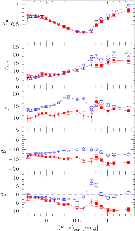
Figure 5: Inverse mean parallax, the asymmetric drift from equation (26b), Oort’s constants (left) and $\tilde{A}-\tilde{B}$, as well as the higher-order terms in the Fourier expansion of ${\overline{\mu}}_{\ell^{\star}}$ (right) obtained for the 19 color bins defined in Table 4.1, after $\kappa$-$\sigma$-clipping, from top to bottom. Both the raw results (circles) and the mode-mixing corrected values (squares) are presented. The vertical dotted lines indicates $(\bv)_{0}=0.75$.

Obviously, there is a significant difference between the raw and mode-mixing corrected values. From our discussion in §5.3.2, we expect the “true” values will be close to the mode-mixing corrected values, but we cannot entirely exclude the raw values as a possibility. We will consider the difference between the raw and mode-mixing corrected values as an upper limit to the systematic error involved. Regardless of this difficulty, several inferences can be made.

First, there is an obvious discontinuity in kinematic properties at $(\bv)_{0}\approx 0.75$. This discontinuity is reflected in all Fourier coefficients of ${\overline{\mu}}_{\ell^{\star}}$ raw or mode-mixing corrected. This is unlikely to be caused predominantly by a difference in distance, since there are no significant correlations between the Fourier coefficients and ${\overline{\pi}}^{-1}$ (not shown). Presumably more important is that these stars span the range in ages where the gradient in the age-velocity relation is large. The unstable nature of the Fourier coefficients in the red-clump region illustrates that it is very difficult to determine the true value of the Oort constants if the ages of the tracer stars are ill-determined.

Figure 6: Mode-mixing coefficients (defined in equation (14)) as estimated from equation (18) for the bins 1 to 7 (open) and 7a to 10 (solid) plotted against the inverse mean parallax estimated via equation (26b).

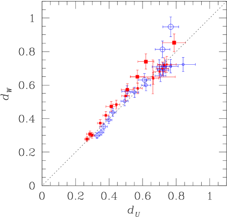
Figure 7: The mean distance estimated from the vertical proper motions (via equation (26b)) versus the distance from the radial proper motions (via equation (26a)). The raw results are represented as circles, the mode-mixing corrected results as squares. The size of the symbols increases with $(\bv)_{0}$.

Second, the asymmetric drift and $\tilde{A}-\tilde{B}$ are only weakly affected by the systematic errors. $\tilde{A}-\tilde{B}\approx 26$ for blue stars (uncorrected for mode-mixing), which is in nice agreement with $\tilde{A}-\tilde{B}=27$ measured from Cepheids by Feast & Whitelock (1997). There is a trend towards larger values for redder stars. At the red end, we again notice the strong discontinuity in the red-clump region $(\bv)_{0}=0.75\pm 0.15$. The red giant bin (#10) has $\tilde{A}-\tilde{B}=26.7\pm 0.7$ and $29.5\pm 1.4$ for the raw and mode-mixing corrected values, respectively. These values are consistent with a Galactic circular frequency of $28\pm 2$ as derived from the proper motion for Sgr A^⋆ (Reid et al., 1999; Backer & Sramek, 1999).

Third, the values for $\tilde{A}$ before and after mode-mixing correction differ by just $1\sigma$ for the red giant stars: $\tilde{A}$ is between $14.2\pm 0.6$ and $12.9\pm 1.1$.

Fourth, except for the very blue stars, there is a large systematic uncertainty for $\tilde{B}$. The red giant bin has $\tilde{B}$ values between –16.6 and –12.5.

Fifth, there are several clear evidences for deviations from axisymmetric equilibrium: non-zero $\tilde{C}$ and $\sin 3\ell$ terms (the latter only for blue stars). Note, in particular, that after mode-mixing correction $\tilde{C}$ has the same sign for all stars.

Finally, while the asymmetric drift is increasing with color independent of whether it has been derived from the raw or mode-mixing corrected coefficients, the curves derived from the $U$ and the $W$ motion differ clearly (not shown). In the latter case, the increase is more gentle and reaches only $v_{\rm a\varphi}\approx 16\,\mbox{${\rm km}\,{\rm s}^{-1}$}$, whereas the $U$-derived coefficients yield $v_{\rm a\varphi}$ 2-4 ${\rm km}\,{\rm s}^{-1}$larger. Note that we do not expect an exact correspondence with the asymmetric drift derived by DB98 because our samples comprise mixes of sub-populations that differ from the local Hipparcos sample, in particular at the red end.

5.3 Mode Mixing

5.3.1 Evidence for Mode Mixing

In Figure 6, we plot the Fourier coefficients $(c_{\pi},s_{\pi})_{m}$, derived from the vertical proper motions utilizing equation (18), versus the inverse mean parallax estimated from the average vertical proper motion via equation (26b). Clearly, these coefficients deviate significantly from zero proving that mode mixing is present and non-negligible, i.e. that the Oort constants obtained without correction are systematically in error. There is a clear dichotomy between main-sequence stars ($\bv<0.8$; open symbols) and non-main-sequence stars ($\bv>0.8$; closed symbols): most mode-mixing coefficients are similar within each color group but differ between them. This indicates different spatial distributions, necessitating separate analyses.

5.3.2 Is our Mode-Mixing Correction Correct?

We have tried to correct for the mode mixing by employing the vertical proper motion and the technique described in §3.2.1 and §3.3.2. However, as discussed in §2.7.3, there are possible caveats in this method, in particular neglecting contributions from higher-order terms (cf. §§2.4 to 2.5). One possible check on the consistency of the results obtained is a comparison of the secular parallaxes estimated from the solar radial and vertical motions via equations (26). Figure 7 compares the estimate ${\overline{\pi}}_{U}^{-1}$, which is affected by mode mixing, with ${\overline{\pi}}_{W}^{-1}$, which is not, before (circles) and after (squares) mode-mixing correction has been applied. Obviously, in both cases a systematic deviation of 5–10% exists between the two estimates, but with opposite signs. An exception are the very early-type stars ($\bv\lesssim 0.2$), which are known to deviate from equilibrium (DB98).

Note that while the deviations from the dotted line increase with distance, they do so less for the mode-mixing corrected results. This indicates that the neglect of higher-order terms, which should introduce systematic errors at large distances, cannot have introduced significant errors.

There are two possible explanations for those differences. First, the ratio $U_{0}/W_{0}$ may be different for this sample than for the more local sample of Hipparcos stars utilized by DB98. In this case, we cannot make any statement, whether our mode-mixing correction works or not.

Second, if $U_{0}/W_{0}$ is equal the DB98 value, we can determine an alternative mode-mixing solution in which we force equality between ${\overline{\pi}}_{U}$ and ${\overline{\pi}}_{W}$. In this case, the radial and tangential proper motions are given by

$${\overline{\mu}}_{U0,W} = U_{0}{\overline{\pi}}_{0}=\frac{U_{0}}{W_{0}}\times{\overline{\mu}}_{W0}$$

$${\overline{\mu}}_{V0,W} = \frac{s_{\pi 2}\times{\overline{\mu}}_{U0,W}-c_{l1}}{1+c_{\pi 2}}$$

from equations (26) and (15a), respectively (we have dropped the latitude dependence). When using these relation for ${\overline{\mu}}_{U0}$ and ${\overline{\mu}}_{V0}$ and solve the mode-mixing equations (15a) directly, we find that the so-determined Oort constants do not differ substantially from our previous mode-mixing corrected values. This indicates that the slight difference between $d_{U}$ and $d_{W}$ does not signify a substantial problem for the mode-mixing scenario.

Since there is overwhelming evidence for the reality of the mode-mixing effect (Figure 6) and the details of the mode-mixing procedure appear to be irrelevant, we conclude that the mode-mixing solutions are robust. In particular, we are confident (and hope to have convinced the reader, too) that the remaining systematic errors of the corrected results are signigicantly smaller than for the raw values. In our subsequent analysis, we will concentrate on the mode-mixing corrected values, but will also show the raw results for comparison.

5.4 Can we make sense of these results?

In §2, we discussed various potential origins for deviations of the measured Oort constants from their “true” values. These deviations, which can be several ${\rm km}\,{\rm s}^{-1}\,{\rm kpc}^{-1}$, originate from departure of the Milky Way from a smooth axisymmetric equilibrium, and may depend on velocity dispersion and mean depth of the stellar population considered. Variations of this order are seen in our results in Figure 5. While a detailled interpretation of the measured variations of the Oort constants is beyond the scope of this paper, we may nontheless examine whether we can single out a dominant cause.

   

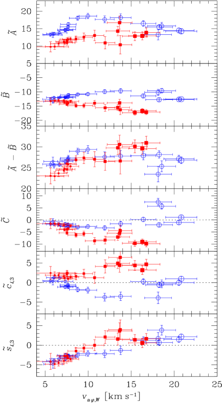
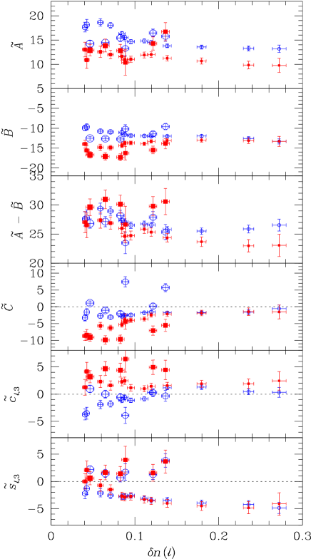
Figure 8: Plotted as a function of the asymmetric drift (left) and the overabundance $\delta n(\ell)$ of stars in direction of spiral-arm tangents (right), we present $\tilde{A},\tilde{B},\tilde{A}-\tilde{B},\tilde{C},c_{\ell,3}$, and $s_{\ell,3}$, from top to bottom. All “Oort constants” depend clearly upon $v_{a\phi}$, most significantly so in the mode-mixing case (squares). The symbol size grows with increasing $(\bv)_{0}$

To disentangle the factors that may contribute to the variation of $\tilde{B}$ with $v_{a\varphi}$, we first compare three sub-populations in Table LABEL:tab:sub_pops. The bluest and reddest stars have similar distances but very different ages, and hence also different velocity dispersions. As the third, we take the reddest main-sequence stars at $(\bv)_{0}\sim 0.6$, which are much nearer.

Properties of some critical sub-populations $(\bv)_{0}$ $d$ $\sigma_{*}$ $v_{a\varphi}$ $f_{Y}$ $\tau$ $\tilde{B}_{r}$ $\tilde{B}_{m}$ $\lesssim 0$ 0.8 15 6 100 0.1 –12 –13 0.6 0.3 36 15 30 8 –10 –16 1.2 0.8 38 17 30 8 –12 –16

Note.— We list approximate values for the intrinsic color, distance, velocity dispersion, asymmetric drift, percentage of young-stars, approximate average age [Gyr], and the raw and mode-mixing corrected Oort’s $B$ ($\tilde{B}_{r}$ and $\tilde{B}_{m}$, respectively).

In fact this is the only relevant property in which they differ significantly from the red giants, see Table LABEL:tab:sub_pops and Figure 5, in particular if one considers the mode-mixing corrected values. A straightforward interpretation is that differences in sample depth are unimportant in causing the differences in the observed Oort constants. This in turn implies that small-scale wiggles of the Galactic velocity field cannot be important either, for otherwise we would expect significantly different results for red MS stars and giants.

We can use the asymmetric drift as a proxy for the mean age and velocity dispersion of a stellar population. Similarly, we may use the overabundance $\delta n(\ell)$ of stars in directions of spiral-arm tangents as a proxy for the fraction of young stars. In Figure 8, we plot the Oort constants measured, including the $m=3$ Fourier coefficients, against our estimate (26b) for the asymmetric drift (left) and $\delta n(\ell)$ (right). The raw data (circles) show only marginal trends with $v_{a\varphi}$, and perhaps even some dichotomy between red main-sequence (small symbols) and giant populations (large symbols). On the other hand, the mode-mixing solutions do not show such a dichotomy but rather tight linear relations between the Oort constants and the asymmetric drift.

A dichotomy is clearly present in the plots versus $\delta n(\ell)$, which arises because the red-clump stars at $\delta n(\ell)\approx 0.13$ have values similar to those of the red giants and unlike those of the blue MS stars at the same $\delta n(\ell)$. Remarkable, however, is that the red MS stars and red giants at $\delta n(\ell)\approx 0.04$ show rather similar values, despite that fact that their average distances differ by a factor $>2$. This is true even for the high-order terms, which argues for their non-zero values not being created by sample-depth effects.

In §2.1 we saw that there should be almost no correlation between asymmetric drift and Oort’s $B$, for the case of axisymmetric equilibrium (and constant sample depth). Thus, the very presence of such a correlation with $v_{a,\varphi}$ as well as non-zero $C$ and $\tilde{s}_{\ell,3}$, argue strongly for non-axisymmetry to be the dominant origin of the observed differences of the Oort constants between stellar subsamples.

Alternatively, non-equilibrium effects may play a role. However, one would then expect a somewhat erratic behaviour, instead of the clean trends seen in the left plot of Figure 8 and also in Figure 5 for the main-sequence stars (i.e. from $(\bv)_{0}=-0.3$ to 0.6).

To summarize, the variations of the Oort constants between the subsamples originate most likely in deviations from axisymmetry, while non-equilibrium effects and small-scale wiggles (deviation from smoothness) seem less important (as do any effects that rely on variations in sample depth). This in turn implies that any interpretation of the Oort constants in terms of the properties of the underlying Galactic potential, the very motivation to undertake studies like this, see §1, cannot be as simple as in Oort’s days.

6 Summary and Conclusion

the Oort constants are defined as the divergence ($K$), vorticity ($B$), azimuthal ($A$) and radial ($C$) shear of the local stellar streaming field of the Milky Way in the limit of vanishing random motions, where all stars move on closed orbits, i.e. circular orbits in case of axisymmetry. The importance of the Oort constants derives from the fact that the dynamics of these closed orbits is directly related to the Galactic gravitational potential, a relation that becomes particularly simple in the axisymmetric case.

The longitudinal proper motion of a star with parallax $\pi$ and radial and azimuthal velocity with respect to the Sun, $U$ and $V$, may be written as

$${\overline{\mu}}_{\ell^{\star}}=-{\rm Re}\,\big{\{}\pi(V+i\,U)\mathrm{e}^{i\ell}\big{\}}.$$ (29)

Assuming that the stellar kinematics and parallaxes are uncorrelated, one finds for the mean longitudinal proper motion

$${\overline{\mu}}_{\ell^{\star}}=-{\rm Re}\,\big{\{}{\overline{\pi}}({\overline{V}}+i\,{\overline{U}})\mathrm{e}^{i\ell}\big{\}}.$$ (30)

The spatial variations of ${\overline{U}}$ and ${\overline{V}}$ are given by the Oort constants, and lead to a $|m|=1$ harmonics $\mathrm{e}^{im\ell}$ in their Fourier expansion. Together with the $\mathrm{e}^{i\ell}$ in (30) this results in $m=0,\,2$ harmonics with amplitudes given by the Oort constants $A$, $B$, and $C$. A similar harmonic dependence is exhibited by the mean radial velocity times parallax, ${\overline{\pi v_{r}}}$. However, stellar parallaxes and radial velocities are difficult to measure and thus the Oort constants are most commonly determined from their effect on the stellar proper motions.

Table 6: The Oort Constants: true and measurable

	symbols	definition and description
(1)	$A$, $B$, $C$, $K$	the Oort constants:
		divergence, vorticity, and shear of the (hypothetical) velocity field ${\boldsymbol{v}}({\boldsymbol{x}})$ due to the closed orbits supported by the Galactic potential
(2)	${\overline{A}}$, ${\overline{B}}$, ${\overline{C}}$, ${\overline{K}}$	the best we can hope to get:
		divergence, vorticity, and shear of the streaming velocity field ${\overline{{\boldsymbol{v}}}}({\boldsymbol{x}})$ of a group of stars
(3)	$\tilde{A}$, $\tilde{B}$, $\tilde{C}$, $\tilde{K}$	what we can actually measure:
		Fourier coefficients of the proper motions measured for a group of stars

6.1 Mode Mixing and Other Problems

The effect of the Oort constants on the stellar proper motions is comparably small. For nearby stars (within ${\sim}1\,\mbox{${\rm kpc}$}$), it is much smaller than the contributions from random stellar motions (i.e. dispersion of $U$ and $V$ in equation (29) and the reflex of the solar motion (i.e. the lowest order in equation (30). Therefore, large proper motion surveys are necessary to extract the Oort constants with reasonable accuracy. There are various, mostly known but neglected, problems arising in this procedure, which are summarized in the footnotes of Table 6.

A fundamental, hitherto apparently overlooked, problem in measuring the Oort constants from proper motion data is what we call mode mixing (point vii in Table 6). In fact, the cause of the problem is rather similar to the very effect one is after. As a spatial variation of $({\overline{U}},{\overline{V}})$, described by the Oort constants, contributes to the $m=0,\,2$ harmonics in the Fourier expansion of ${\overline{\mu}}_{\ell^{\star}}$, so does a variation of ${\overline{\pi}}$. This contribution is indistinguishable from that due to the Oort constants itself.

For a typical situation, already a variation in the mean parallax of only 10% results in a contribution of a few ${\rm km}\,{\rm s}^{-1}\,{\rm kpc}^{-1}$, larger than any other source of uncertainty in the Oort constants. Such a variation of ${\overline{\pi}}$ is not anticipated from a smooth exponential disk. However, that seems to be a bad description of the actual situation for a typical stellar sample. First, the stellar distribution is inhomogeneous, in particular for early-type stars, which are predominantly situated in spiral arms. Secondly, even if the underlying density is rather smooth, extinction inevitable leads to significant inhomogeneities in any actual stellar sample.

In order to correct for the mode mixing, one needs an unbiased estimate of the variations of ${\overline{\pi}}$ with $\ell$. For low-latitude samples, such an estimate may be provided from the latitudinal proper motion $\mu_{b}$, the mean of which at $b=0$ should be given by ${\overline{\mu}}_{b}={\overline{\pi\,W}}$. Here, $W$ is the vertical stellar motion with respect to the Sun. If (1) $\pi$ and $W$ are uncorrelated, and (2) ${\overline{W}}$ is constant with $\ell$, then we can directly measure the relative variations of ${\overline{\pi}}$. A local stellar warp would invalidate both these assumptions, and, hence, one would best not rely on them, but use an independent and unbiased, though not necessarily very accurate, distance estimate for the individual stars. Unfortunately, such an estimate is not currently available – note that the photometric parallax is ill-suited for this purpose.

There is also a more technical issue that we want to emphasize. The standard way to determine the Oort constant from proper motion surveys used to be a least-square fit of the data to a functional form that just accounts for the reflex of the solar motion and the Oort constants, i.e. does not allow for higher-order Fourier modes. This essentially is a parametric fit, and as such will give biased estimates for the parameters if the data are not well described by the functional form fitted. In our analysis, we allow for high-order terms, and found indeed that these are non-negligible. We also restricted our analysis to low latitude stars for three reasons: (i) restricting the latitude to a narrow range, we do not need to account for possible latitudinal variations of the mean proper motions; (ii) only at low $b$ can we use the latitudinal proper motion to correct for mode mixing; and (iii) the Oort constants are strictly defined only for closed, i.e. planar, orbits. Moreover, most disk stars in sufficiently deep samples are predominantly at low latitudes anyway. A disadvantage of low latitude stars is that extinction is largest and most patchy in this region, so that the variation of ${\overline{\pi}}$ with longitude is likely to be maximal here.

6.2 Longitudinal Number-Density Variations

Before analyzing the proper motions of the low-latitude ($|b|<5.73\arcdeg$) stars from the ACT/Tycho-2 catalogs, we first considered their longitudinal distribution as a function of color. For the bluest stars in the sample ($\bv\approx{-}0.1$), this distribution shows three narrow peaks in the direction of the nearby spiral-arm tangents.

Next, we quantified the over-abundance of stars at the longitudes associated with these three peaks. This over-abundance may be interpreted as a measure for the importance of stars in spiral arms. In fact, we use the relative over-abundance $\delta n(\ell)$ to estimate the fraction of young stars in our color bins. These estimates compare well with estimates based on the star-formation history. With increasing color along the main sequence, $\delta n(\ell)$ decreases, but never diminishes completely.

At colors redder than $(\bv)_{0}\approx 0.75$, sub-giant, red-clump, giant and super-giant stars dominate the sample. Interestingly, at about $(\bv)_{0}=0.9$, i.e. for red-clump stars, the over-abundance of stars at the peak-longitudes increases back to the value for early-type stars as blue as $(\bv)_{0}\approx 0.25$. This can be explained by the about equal duration of the horizontal-branch phase for stars of all masses ${\lesssim}2\,{\rm M}_{\odot}$, making the red clump a strange mixture of stars of all ages. As a consequence, any external observer of the Milky Way using some red pass band which allows for red-clump stars to contribute significantly, would see a spiral pattern considerably stronger than that of the underlying old-disk population, which essentially represents the stellar mass distribution.

For yet redder colors, i.e. beyond $(\bv)_{0}\approx 1.2$, our measure for the importance of spiral structure drops again, but not quite as low as for the dwarfs at $(\bv)_{0}\approx 0.6$. This is because the duration of the giant-branch phase is shorter for more massive and hence younger stars, such that the giants are rather old on average.

6.3 The Oort Constants

The significant non-uniformity of the longitudinal stellar distribution strongly hints towards inhomogeneity in the spatial distribution of the sample stars. Thus, longitudinal parallax variations and hence a confusion of the Oort constants by mode mixing with the solar reflex motion is expected and observed. In the previous sections we have presented evidence that the mode-mixing corrected values are likely to be close to the “true” Oort constants. We thus present the mode-mixing results below.

The absolute values of the Oort constants are small for young, blue stars. Extrapolating to zero asymmetric drift we find (in ${\rm km}\,{\rm s}^{-1}\,{\rm kpc}^{-1}$).

$$\mbox{young MS stars:\hskip 20.00003pt}\begin{array}[]{r@{\,=\,}r}A&9.6,\\ B&-11.6,\\ A-B&21.1,\\ C&0.4,\\ s_{\ell,3}&-6.7,\\ c_{\ell,3}&-0.1,\end{array}$$ (31)

with internal errors of about 0.5 ${\rm km}\,{\rm s}^{-1}\,{\rm kpc}^{-1}$. The oldest stars in our samples, giants with $(\bv)_{0}\gtrsim 1.2$, have significantly larger Oort constants. At $v_{a\varphi}=18$ we get:

$$\mbox{old red giants:\hskip 20.00003pt}\begin{array}[]{r@{\,=\,}r}A&15.9,\\ B&-16.9,\\ A-B&32.8,\\ C&-9.8,\\ s_{\ell,3}&2.6,\\ c_{\ell,3}&4.3,\end{array}$$ (32)

with internal errors of about 1.2 ${\rm km}\,{\rm s}^{-1}\,{\rm kpc}^{-1}$, and where 2 ${\rm km}\,{\rm s}^{-1}\,{\rm kpc}^{-1}$has already been added to the $A$ value of the giants in order to correct for the reduction by the asymmetric drift (cf. §2.1). The external errors are harder to estimate.

Our values for $A$ and $B$ for the old stars are somewhat unusual, which is largely due to our mode-mixing correction. Using the raw Fourier coefficients whereby ignoring this effect, one finds for the giants more conventional numbers, in particular $A_{\mathrm{raw}}\approx 14,B_{\mathrm{raw}}\approx{-}12.5$ and $C_{\mathrm{raw}}\approx 0$.

The values for the Oort constants for the young and old stars derived with the mode-mixing corrections are not inconsistent with previous determinations. In part this arises due to the fact that most previous work has applied parametric methods to derive the Oort constants, in part because published results still have significant uncertainties, and partly because all these values are uncertain due to the various systematic effects discussed above.

A relatively large value for $\Omega$ has been found from the longitudinal proper motion of Sgr A$\!{}^{\star}$ (if Sgr A$\!{}^{\star}$ is at rest in the Galactic center). In that case, $\Omega\equiv A-B=28\pm 2$ (Backer & Sramek, 1999; Reid et al., 1999). Even larger values for $A-B(\approx 31.5$) have been reported by Méndez et al. (1999) and Miyamoto & Zhu (1998), based on absolute proper motions derived from the Southern Proper Motion Program and the Hipparcos Catalogue, respectively (note, however, hat these two works have employed the classical parametric $\mu_{\ell}=B+A\cos 2\ell$ description of Galactic rotation). All of these results are consistent with our determinations for old stars (32).

6.4 What can be learned from the Oort constants?

To our knowledge, the linear dependence of the Oort constants on asymmetric drift is a new discovery. It is worth noting here, that while such a dependence was in principal expected already by Oort, our measurements are inconsistent with expectations from axisymmetric models for the Milky Way.

The non-zero $\tilde{s}_{\ell,3}$ value for young stars clearly shows that non-axisymmetry is present amongst these stars, which given their affiliation with spiral arms is not surprising at all. While for older stars $\tilde{s}_{\ell,3}$ diminishes, another indicator of non-axisymmetry, Oort’s $C$, becomes very significantly non-zero. For other sitations than axisymmetry, predictions for the values expected for the Oort constants are considerably involved and require detailled modelling. This is true especcially, if effects of the sample depth and velocity distribution are to be taken into account.

As indicated by the imprints of the Galactic bar on the local velocity distribution measured from Hipparcos data (Dehnen, 1998), the Sun lies just outside the outer Lindblad resonance (OLR) of the bar (Dehnen, 2000). This is exactly the place where the bar is expected to most strongly distort the local kinematics. In particular, stars from inside the OLR should produce $C<0$, and in a deep sample the number of such stars should be larger than in a very local volume. Indeed, when analyzing only the stars brighter than $V_{T}=10.5$, $C$ rises to $-7.5$, i.e. the effect is weaker. Thus, the value of $C$ might arise from contributions of stars from inside the OLR. Mühlbauer & Dehnen (2003) have analysed the effect of the Galactic bar on the stellar kinematics in the outer disk and find that larger a velocity dispersion, as for the red giants, tends to shift the “effective radius” of resonance outwards. They also find weaker distortions to the local $C$ than our result.

Another intriguing possibility is that asymmetries in the stellar distribution function arising from a (or more) satellite merger, like that of the Sgr dwarf, contributes to the apparent anomalies. Note that there appear to be asymmetries in the local number of thick disk/inner halo stars (Larsen & Humphreys, 1996; Parker, Humphreys, & Larsen, 2001).

Further work is needed to investigate whether such values can be explained when (1) considering sample-depth effects, i.e. simulating the actual data-taking and measurement process, (2) residual non-equilibrium effects from minor mergers, (3) and accounting for the additional non-axisymmetric forcing of triaxial halo, elliptical disk (e.g., Kuijken & Tremaine, 1994), or spiral arms. This latter option is interesting as the Sun resides also close to the co-rotation radius of the spiral pattern (e.g., Lin, Yuan & Shu, 1969; Mishurov Pavlovskaia & Suchkov, 1979), where one would expect its forcing to be most efficient.

6.5 Resumé

The very concept of the Oort constants is originally based on the idealization of the Milky Way being axisymmetric with almost circular stellar orbits. Similarly, in determining the Oort constants from stellar proper motions one has usually relied, at least implicitly, on the smoothness of the spatial distribution of the sampled stars. At Oort’s time, the deviations of reality from these ideals have been of second order compared to the internal uncertainties due to the low accuracy and sparse samples. However, with ever increasing accuracy and larger samples, these deviations inevitably become significant. Nonetheless, they have been largely ignored so far, resulting in significant systematic errors. The presence of such errors is reflected in the previous determinations of the Oort constants listed by Kerr & Lynden-Bell (1986), whose scatter exceeds the typical internal errors.

In this paper, we (1) tried to explain the possible deviations from the above ideal and the resulting systematics, in particular when using large proper motion surveys, and (2) tried as far as possible both to avoid and correct for them in our application to the ACT/Tycho-2 catalogs. Avoiding uncontrollable systematics lead us to exclude the results from either young, high-latitude, or nearby stars. Thus, the most reliable results reported in the present study are those for the (mainly old) giants in the Galactic plane, for which there are two main sources of systematics: the asymmetric drift and mode mixing. While the first problem was already known to Oort (1928), the second is not mentioned in previous determinations of the Oort constants from proper motions. Our correction for this latter effect using the stars’ vertical proper motions changes the Oort $A$, $B$, and $C$ from more conventional numbers to the values reported in equation (32) for old stars.

We hope that possible future space missions such as FAME, DIVA, SIM, and GAIA will dramatically improve both the quality and amount of the data, yielding highly accurate five- or even six-dimensional phase-space coordinates for millions of stars throughout the Milky Way. With such data, many of the hitherto unpleasant deviations from Oort’s idealized Galaxy will become clearly apparent and must be dealt with properly. Very likely, the classical deductive way of ‘measuring’ the Oort constants directly from the data, becomes hardly viable then. Instead, a detailed analysis is needed which compares the data with predictions from sophisticated dynamical models incorporating the Galactic bar, spiral structure, non-equilibrium effects such as moving groups, and other deviations from Oort’s ideal Milky Way. In fact, these deviations, which plague our current determination of the Galactic potential, are likely to constrain the models significantly leading eventually to a much enhanced understanding of the structure and formation of our host galaxy.

One datum that is very important to the study of the dynamics of the Milky Way will not be collected by the future space-based astrometric missions. The lack of approximate ages of the individual tracer stars will seriously compromise the study of the dynamical evolution of the Galaxy. We have already noted that the interpretation of the proper motions of certain kinds of stars (the red-clump region) is hampered due our inability to associate these stars with either young or old stellar populations.

We anticipate that age-related effects will become an important limitation to the interpretation of the space-based astrometric data. Age information would allow us to study many topics related to the formation and evolution of the Milky Way, such as (1) the (relative) ages of various stellar components, (2) the temporal variation of the star formation activity, (3) the minor-merger history (through distinct features in the age-velocity relation). Such studies would turn the Milky Way into an important benchmark galaxy, not only at the present, but also at cosmologically interesting epochs.

References

- Amaral & Lépine (1997) Amaral, L.H. & Lépine, J.R.D. 1997, MNRAS, 286, 885
- Amaral et al. (1996) Amaral, L.H., Ortiz, R., Lépine, J.R.D., Maciel, W.J. 1996, MNRAS, 281, 339
- Backer & Sramek (1999) Backer D.C., Sramek R.A. 1999, ApJ, 524, 805
- Binney et al. (1997) Binney J.J., Dehnen W., Houk N., Murray C.A., Penston M.J. 1997, ESA SP-402, 473
- Binney & Tremaine (1987) Binney J.J., Tremaine, S. 1987, Galactic Dynamics, Princeton Univ. Press, Princeton
- Chandrasekhar (1942) Chandrasekhar S. 1942, Principles of Stellar Dynamics, Univ. of Chicago Press, Chicago
- Chen et al. (1998) Chen, B., Vergely, J.L., Valette, B., Carraro, G. 1998 A&A, 336, 137
- Clube (1972) Clube S.V.M. 1972, MNRAS, 159, 289
- Cole (1998) Cole A.A. 1998, ApJ, 500, L137
- Corbin & Urban (1988) Corbin T.E., Urban S.E. 1988, IAU Symp. 133 Mapping the Sky, ed. S. Debarbat J.A., Eddy H.K., Eichhorn A.R., Upgren, Kluwer, Dordrecht, 287
- Crézé & Mennessier (1973) Crézé, M., Mennessier, M.O. 1973, A&A, 27, 281
- Dehnen & Binnez (1998) Dehnen W., Binney J.J. 1998, MNRAS, 298, 387, DB98
- Dehnen (1998) Dehnen W. 1998, AJ, 115, 2384
- Dehnen (1999) ——–. 1999, ApJ, 525, L35
- Dehnen (2000) ——–. 2000, AJ, 119, 800
- Drimmel (2000) Drimmel, R. 2000, A&A, 358, L13
- Drimmel & Spergel (2001) Drimmel, R., Spergel, D. 2001, ApJ, 556, 181
- Eichhorn (1974) Eichhorn H. 1974, Astronomy of Star Positions, Ungar, New York
- Englmaier & Gerhard (1999) Englmaier P., Gerhard O.E. 1999, MNRAS, 304, 512
- ESA (1997) ESA 1997, The Hipparcos and Tycho Catalogues, ESA SP-1200
- Feast & Whitelock (1997) Feast M.W., Whitelock P.A. 1997, MNRAS, 291, 683
- Fricke (1971) Fricke, W. 1971, A&A, 13, 298
- Fux (1999) Fux R. 1999, A&A, 345, 787
- Girardi et al. (1998) Girardi L., Groenewegen M.A.T., Weiss A., Salaris M. 1998, MNRAS, 301, 149
- Gómez & Mennessier (1977) Gómez A., Mennessier M.O. 1977, A&A, 54, 113
- Hanson (1987) Hanson R.B. 1987, AJ, 94, 409
- Hog et al. (2000b) Hog, E. et al. 2000b, A&A, 357, 367
- Hog et al. (2000a) Hog, E. et al. 2000a, A&A, 355, L27
- Hog et al. (1998) Hog, E., Kuzmin, A., Bastian, U., Fabricius, C., Kuimov, K., Lindgren, L., Makarov, V. V., Roeser, S. 1998, A&A, 335L
- Jeans (1922) Jeans J.H. 1922, MNRAS, 82, 122
- Jenkins (1992) Jenkins, A. 1992, MNRAS, 257, 620
- Kalnajs (1991) Kalnajs A.J. 1991, in Sundelius B., ed., Dynamics of Disc Galaxies, Göteborgs University, p. 323
- Kapteyn & van Rhijn (1920) Kapteyn, J.C., van Rhijn, P.J. 1920, ApJ, 53, 23
- Kapteyn (1922) Kapteyn, J.C. 1922, ApJ, 55, 302
- Kerr & Lynden-Bell (1986) Kerr F.J., Lynden-Bell D. 1986, MNRAS, 221, 1023
- Kovalevsky et al. (1997) Kovalevsky J. et al. 1997, A&A, 323, 620
- Kuijken & Tremaine (1994) Kuijken K., Tremaine S. 1994, ApJ, 421, 178
- Larsen & Humphreys (1996) Larsen, J.A., Humphreys, R.M. 1996, AJ, 468, 99
- Lewis & Freeman (1989) Lewis J.R., Freeman K.C. 1989, AJ97139
- Lin, Yuan & Shu (1969) Lin, C.C., Yuan, C., Shu, F.H. 1969, ApJ, 155, 721
- Lindblad (1927) Lindblad, B. 1927, MNRAS, 87, 553
- Lindgren & Kovalevsky (1995) Lindgren, L., Kovalevsky, J. 1995, A&A, 304, 189
- Mayor (1974) Mayor M. 1974, A&A, 32, 321
- Méndez et al. (1999) Méndez, R. A., Platais, I., Girard, T. M., Kozhurina-Platais, V. & van Altena, W.F. 1999, ApJ, 524, L39
- Milne (1935) Milne E.A. 1935, MNRAS, 95, 560
- Mishurov Pavlovskaia & Suchkov (1979) Mishurov, I. N., Pavlovskaia, E. D. & Suchkov, A. A. 1979, AZh, 56, 268
- Mishurov & Zenina (1999) Mishurov, Yu. N., Zenina, I.A. 1999, A&A, 341, 81
- Miyamoto & Soma (1993) Miyamoto, M., Soma, M. 1993, AJ, 105, 691
- Miyamoto & Zhu (1998) Miyamoto, M., Zhu, Z. 1998, AJ, 115, 1483
- Mühlbauer & Dehnen (2003) Mühlbauer, G., Dehnen, W., 2003, A&A, submitted
- Ogorodnikov (1932) Ogorodnikov, K.F. 1932, Z. Astrophys., 4, 190
- Olling & Merrifield (1998) Olling R.P., Merrifield M.R. 1998, MNRAS, 297, 943
- Oort (1927a) Oort J.H. 1927a, Bull. Astr. Inst. Neth., 3, 275
- Oort (1927b) ——–. 1927b, Bull. Astr. Inst. Neth., 4, 79
- Oort (1928) ——–. 1928, Bull. Astr. Inst. Neth., 4, 269
- Parker, Humphreys, & Larsen (2001) Parker, J.E., Humphreys, R.M., Larsen, J.A. 2001, BAAS, 199, #91.05
- Pont, Mayor & Burki (1994) Pont F., Mayor M., Burki G. 1994, A&A, 285, 415
- Reid et al. (1999) Reid M.J., Readhead A.C.S., Vermeulen R.C., Treuhaft R.N. 1999, ApJ, 524, 816
- Seidel, Demarque & Weinberg (1987) Seidel E., Demarque P., Weinberg D. 1987, ApJS, 63, 917
- Shapley (1918) Shapley H. 1918, ApJ, 48, 154
- Urban, Wycoff, & Makarov (2000) Urban, S. E., Wycoff, G. L., & Makarov, V. V. 2000, AJ, 120, 501
- Urban, Corbin & Wycoff (1998) Urban S.E., Corbin T.E., Wycoff G.L. 1998, AJ, 115, 2161
- Urban et al. (1998) Urban S.E., Corbin T.E., Wycoff G.L., Martin J.C., Jackson E.S., Zacharias M.I., Hall D.M. 1998, AJ, 115, 1212
- Vallée (1995) Vallée, J.P. 1995, ApJ, 454, 119