Towards a self-consistent relativistic model of the exterior gravitational field of rapidly rotating neutron stars

Abstract

We present a self-consistent, relativistic model of rapidly rotating neutron stars describing their exterior gravitational field. This is achieved by matching the new solution of Einstein’s field equations found by Manko et al. [2000] and the numerical results for the interior of neutron stars with different equations of state calculated by Cook et al. [1994]. This matching process gives constraints for the choice of the five parameters of the vacuum solution. Then we investigate some properties of the gravitational field of rapidly rotating neutron stars with these fixed parameters.

1 Introduction

Accretion on to neutron stars is primarily determined by their exterior gravitational field for which an analytical description is preferable to a numerical one. The solutions of Einstein’s field equations suitable for Black Holes as the Schwarzschild- and the Kerr-metric do not hold for neutron stars because those have a solid surface and are therefore oblate when rapidly rotating. The second difficulty is the possible existence of an intrinsic magnetic field. A new solution has been strongly needed including the two parameters of the Kerr-metric, mass and angular momentum, and three additional ones, the mass quadrupole moment due to the oblateness of the star, the electric charge (which is of no importance for astrophysical objects) and the magnetic dipole moment. After more than ten years of work Manko et al. [2000] found a space-time meeting all criteria.

These parameters are in a mathematical sense formally independent, but in an astrophysical sense, the mass quadrupole moment is a function of the mass and the angular momentum. To find these dependencies we use numerical results found by Cook et al. [1994]. They solved the general relativistic structure equations for an axisymmetric rotating star for 14 different equations of state (EOS) and three sequences and presented certain quantities for the stars in a tabulated form for five of them. By comparing those with the analytical values we get correlations for the parameters of the new solution.

This was also done by Sibgatullin & Sunyaev [1998], but with another metric [1994] and only three EOS with low stiffness. These authors investigated their found models in further publications (the most recent is Sibgatullin & Sunyaev [2000]). This metric, however, did not permit the rational function representation – the reason why Manko et al. continued their search for a new solution – and could not be written in a concise form which is more useful for analytical examinations. Furthermore the same procedure – but in opposite order – was done for this new metric extended to all five EOS and all three sequences.

With fixed parameters this new solution is highly useful to improve the models of rapidly rotating neutron stars e.g. in accretion disc calculations for which the Schwarzschild- or Kerr-metric are still used at this time. These introduce large errors because of their significant deviations to real neutron stars due to symmetry simplifications which are now not necessary anymore.

2 The general exterior field of rotating neutron stars

Starting with the most general form of a stationary axisymmetric metric, found by Papapetrou [1953],

$$ds^{2}=f\,(dt-w\,d\phi)^{2}-f^{-1}[\,e^{2\gamma}\,(d\rho^{2}+dz^{2})+\rho^{2}\,d\phi^{2}],$$ (1)

where $\rho$ and $z$ are quasi-cylindrical Weyl-Papapetrou-coordinates and $f$, $w$ and $\gamma$ are functions independent of $\phi$ and $t$, Ernst [1968] found that Einstein’s equations reduce to the form

$$(Re\,\mathcal{E}+|\Phi|^{2})\nabla^{2}\mathcal{E} = (\nabla\mathcal{E}+2\Phi^{*}\nabla\Phi)\cdot\nabla\mathcal{E}$$

$$(Re\,\mathcal{E}+|\Phi|^{2})\nabla^{2}\Phi = (\nabla\mathcal{E}+2\Phi^{*}\nabla\Phi)\cdot\nabla\Phi,$$ (2)

after introducing the two complex potentials $\mathcal{E}$ and $\Phi$ and their complex conjugates $\mathcal{E}^{*}$ and $\Phi^{*}$ as

$$\mathcal{E}=(f-|\Phi|^{2})+i\varphi\qquad\Phi=A_{t}+i\varphi^{\prime},$$ (3)

$\varphi$ and $\varphi^{\prime}$ are defined by

$$\rho^{-1}f^{2}\nabla w-2\hat{n}\times Im(\Phi^{*}\nabla\Phi) = \hat{n}\times\nabla\varphi$$

$$\rho^{-1}f(\nabla A_{\phi}-w\nabla A_{t}) = \hat{n}\times\nabla\varphi^{\prime}$$ (4)

with the $t$- and $\phi$-components $A_{t}$ and $A_{\phi}$ of the electromagnetic four-potential and the unit-vector in azimuthal direction $\hat{n}$. If the Ernst-potentials are known, the functions $f$, $w$ and $\gamma$ can be directly calculated from

$$f = Re\mathcal{E}+\Phi\Phi^{*}$$

$$w_{,\rho} = -\rho f^{-2}[\varphi_{,z}+2\,Im(\Phi^{*}\Phi_{,z})]$$

$$w_{,z} = \rho f^{-2}[\varphi_{,\rho}+2\,Im(\Phi^{*}\Phi_{,\rho})]$$

$$\gamma_{,\rho} = \frac{1}{4}\rho f^{-2}[(\mathcal{E}_{,\rho}+2\,\Phi^{*}\Phi_{,\rho})(\mathcal{E}_{,\rho}^{*}+2\,\Phi\Phi_{,\rho}^{*})$$

$$-(\mathcal{E}_{,z}+2\,\Phi^{*}\Phi_{,z})(\mathcal{E}_{,z}^{*}+2\,\Phi\Phi_{,z}^{*})]$$

$$-\rho f^{-1}(\Phi_{,\rho}\Phi_{,\rho}^{*}-\Phi_{,z}\Phi_{,z}^{*})$$

$$\gamma_{,z} = \frac{1}{2}\rho f^{-2}Re[(\mathcal{E}_{,\rho}+2\,\Phi^{*}\Phi_{,\rho})(\mathcal{E}_{,z}^{*}+2\,\Phi\Phi_{,z}^{*})]$$ (5)

$$-2\rho f^{-1}Re(\Phi_{,\rho}^{*}\Phi_{,z}).$$

The two Ernst-equations are solved by simple integral equations [1991] which introduce the axis data of the Ernst-potentials $e(z)=\mathcal{E}(\rho=0,z)$ and $f(z)=\Phi(\rho=0,z)$:

$$\mathcal{E}=\frac{1}{\pi}\int\limits^{1}_{-1}\frac{e(\xi)\mu_{1}d\sigma}{\sqrt{1-\sigma^{2}}}\qquad\Phi=\frac{1}{\pi}\int\limits^{1}_{-1}\frac{f(\xi)\mu_{1}d\sigma}{\sqrt{1-\sigma^{2}}},$$ (6)

where $\mu_{1}$ has to satisfy

$$\int\limits^{1}_{-1}\!\!\!\!\!\!\!\!\;-\,\,\,\frac{\mu_{1}(\sigma)\,(\tilde{e}(\eta)+e(\xi)+2\tilde{f}(\eta)f(\xi))\,d\sigma}{(\xi-\eta)\,\sqrt{1-\sigma^{2}}} = 0$$

$$\int\limits^{1}_{-1}\frac{\mu_{1}(\sigma)\,d\sigma}{\sqrt{1-\sigma^{2}}} = \pi$$ (7)

with $\eta=z+i\rho\tau$, $\xi=z+i\rho\sigma$, $\tilde{e}(\xi)=\bar{e}(\bar{\xi})$, $\tau,\sigma\in[-1,1]$. In the first integral the Cauchy principal value has to be calculated. These new functions can be expressed as a multipole expansion of the mass-, angular momentum-, electric and magnetic field-distribution

$$\mathcal{E}=\frac{1-\xi}{1+\xi}\qquad\Phi=\frac{q}{1+\xi}$$ (8)

$$\xi(\rho=0) = \sum^{\infty}_{n=0}m_{n}z^{-(n+1)}$$

$$q(\rho=0) = \sum^{\infty}_{n=0}q_{n}z^{-(n+1)}.$$ (9)

The physical multipole moments are the real (mass multipoles) and imaginary (angular momentum multipoles) part of $m_{n}$ and the real (electric multipoles) and imaginary (magnetic multipoles) part of $q_{n}$.

To derive a new exact analytical solution of Einstein’s equations one starts with an ansatz of $e(z)$ and $f(z)$, checks whether the solution has the wanted parametrisation of the multipole moments and performs the cumbersome but straight-forward calculation of the metric functions $f$, $w$ and $\gamma$.

Different authors (e.g. Aguirregabaria et al. [1993], Manko et al. [1994]) made an effort to find a new solution involving five parameters representing mass, angular momentum, charge, magnetic dipole moment and mass quadrupole moment of the star which can be expressed with relatively simple rational functions. After more than ten years and several ansatzes such a solutions was found [2000] starting with

$$e(z) = \frac{(z-m-ia)\,(z+ib)+d-\delta-ab}{(z+m-ia)\,(z+ib)+d-\delta-ab}$$

$$f(z) = \frac{Qz+i\mu}{(z+m-ia)\,(z+ib)+d-\delta-ab}$$ (10)

with

$$\delta = \frac{\mu^{2}-m^{2}b^{2}}{m^{2}-(a-b)^{2}-Q^{2}}$$

$$d = \frac{1}{4}\,[m^{2}-(a-b)^{2}-Q^{2}].$$ (11)

After checking the multipole moments one finds that $m$ is the mass, $a$ the specific angular momentum, $Q$ the charge and $\mu$ the magnetic dipole moment (if $Q=0$). The parameter $b$ is no physical quantity, but is related to the mass quadrupole moment. For comparison the functions $e(z)$ and $f(z)$ of the Schwarzschild- and the Kerr-solution are

$$e(z)=\frac{z-m}{z+m}=1-\frac{2m}{z+m}\qquad f(z)=0$$ (12)

$$e(z)=\frac{z-m+i\,a}{z+m+i\,a}\qquad f(z)=0.$$ (13)

To be able to write the metric function in a rational form it is convenient to introduce general spheroidal coordinates by

$$x=\frac{1}{2\kappa}(r_{+}+r_{-})\qquad y=\frac{1}{2\kappa}(r_{+}-r_{-})$$ (14)

with $r_{\pm}=\sqrt{\rho^{2}+(z\pm\kappa)^{2}}$ and $\kappa=\sqrt{d+\delta}$. The metric then becomes

$$ds^{2} = f\,(dt-w\,d\phi)^{2}-\kappa^{2}f^{-1}\Bigl{[}e^{2\gamma}\,(x^{2}-y^{2})\Bigl{(}\frac{dx^{2}}{x^{2}-1}$$ (15)

$$+\frac{dy^{2}}{1-y^{2}}\Bigr{)}+(x^{2}-1)(1-y^{2})d\phi^{2}\Bigr{]}$$

and the functions are

$$f=\frac{E}{D}\qquad e^{2\gamma}=\frac{E}{16\kappa^{8}(x^{2}-y^{2})^{4}}\qquad w=\frac{-(1-y^{2})F}{E}$$

with

$$E = \{4[\kappa^{2}(x^{2}-1)+\delta(1-y^{2})]^{2}+(a-b)$$

$$[(a-b)(d-\delta)-m^{2}b+Q\mu](1-y^{2})^{2}\}^{2}$$

$$-16\kappa^{2}(x^{2}-1)(1-y^{2})\{(a-b)[\kappa^{2}(x^{2}-y^{2})$$

$$+2\delta y^{2}]+(m^{2}b-Q\mu)y^{2}\}^{2}$$

$$D = \{4(\kappa^{2}x^{2}-\delta y^{2})^{2}+2\kappa mx[2\kappa^{2}(x^{2}-1)$$

$$+(2\delta+ab-b^{2})(1-y^{2})]+(a-b)[(a-b)(d-\delta)$$

$$-m^{2}b+Q\mu](y^{4}-1)-4d^{2}\}^{2}+4y^{2}\{2\kappa^{2}(x^{2}-1)$$

$$[\kappa x(a-b)-mb]-2mb\delta(1-y^{2})+[(a-b)$$

$$(d-\delta)-m^{2}b+Q\mu](2\kappa x+m)(1-y^{2})\}^{2}$$

$$F = 8\kappa^{2}(x^{2}-1)\{(a-b)[\kappa^{2}(x^{2}-y^{2})+2\delta y^{2}]$$ (17)

$$+y^{2}(m^{2}b-Q\mu)\}\{\kappa mx[(2\kappa x+m)^{2}-2y^{2}(2\delta+ab$$

$$-b^{2})-a^{2}+b^{2}-Q^{2}]-2\kappa^{2}Q^{2}x^{2}-2y^{2}(4\delta d$$

$$-m^{2}b^{2})\}+\{4[\kappa^{2}(x^{2}-1)+\delta(1-y^{2})]^{2}$$

$$+(a-b)[(a-b)(d-\delta)-m^{2}b+Q\mu]$$

$$(1-y^{2})^{2}\}(4(2\kappa mbx+2m^{2}b-Q\mu)$$

$$[\kappa^{2}(x^{2}-1)+\delta(1-y^{2})]+(1-y^{2})$$

$$\{(a-b)(m^{2}b^{2}-4\delta d)-(4\kappa mx+2m^{2}$$

$$-Q^{2})[(a-b)(d-\delta)-m^{2}b+Q\mu]\}).$$

Mathematically, the five parameters of this solution are independent. To make it applicable for astrophysical purposes and to describe astrophysical configurations, one needs to find constraints for the choice of and the relations between some of these parameters. Those can only be found by matching the exterior solution with existing models for the interior of neutron stars.

3 The Interior of neutron stars

Until now, the knowledge of the composition of the interior of neutron stars is very poor. A large zoo of different EOS exists to describe all possible ingredients of the star and the interactions of these particles. Before the right EOS can be singled out by observations, i.e. determining the mass-radius-relation by e.g. measuring the cooling curve of neutron stars, the basic structure equations for rotating, axisymmetric stars – similar to the Oppenheimer-Volkoff-equations for spherical stars – have to be solved numerically for each model. Cook et al. [1994] performed these calculations for 14 different EOS with a modified variation of the KEH-Code [1989] and tabulated several quantities for five of them representing the whole range of stiffness (A, AU, FPS, L, M; see table 1, Cook et al. [1994] and references therein). For further informations on different numerical methods see e.g. Ansorg et al. [2002] and references therein.

Table 1: Equations of state, used in Cook et al. [1994]

EOS	Description
A	Reid soft core, adapted to nuclear matter
AU	Argonne V14 + Urbana VII
FPS	Urbana V14 + Three Nuclei Interaction
L	Nuclear attraction due to scalar exchange
M	Nuclear attraction due to pion exchange
	(Tensor interaction)

For each EOS these authors computed models for three star sequences: first the normal sequence (NS) of stars whose masses are below the maximum mass of non-rotating stars, second the maximum mass normal sequence (MM) of stars with the maximum mass of non-rotating stars and third the supramassive sequence (SM) of stars whose masses exceed the maximum mass of non-rotating stars. These numerical values can be compared with the analytically derived ones to adjust the free parameters. The following fitting procedure was performed for all five equations of state and all three sequences.

There exists a newer EOS including more effects of nuclear and particle physics (Glendenning & Weber [2001] and references therein), but unfortunately the analog analysis of Cook et al. [1994] has not yet been done. Perhaps this modern EOS describes the interior of neutron stars in a better way than the older EOS considered by Cook et al., then the same fitting procedure performed with this EOS would give more physically meaningful results. More observations are needed to clear this point.

4 Fitting the free parameters

4.1 The gravitational redshift

One of the quantities tabulated in Cook et al. [1994] is the gravitational redshift photons experience being emitted forward ($Z_{f}$) and backward ($Z_{b}$) with respect to the rotation direction at the equator. The same can be easily calculated for this analytical solution. For photons which are emitted at the equator in forward (backward) direction with respect to the rotational direction the four-momentum has the form

$$p^{\mu}=\textrm{const.}\,\times\,[\,\xi_{(t)}^{\mu}+\frac{f}{fw\pm\rho}\,\xi_{(\phi)}^{\mu}\,]$$ (18)

with the Killing-vectors $\xi_{(t)}^{\mu}$ and $\xi_{(\phi)}^{\mu}$. The frequency is calculated by

$$\omega_{E}=p_{\mu}\,u^{\mu},$$ (19)

where the fluid four-velocity on the equator is

$$u^{\mu}=\frac{f^{-1/2}}{\sqrt{1-v^{2}}}\,(\xi_{(t)}^{\mu}+\Omega\,\xi_{(\phi)}^{\mu})$$ (20)

and the fluid velocity measured by a ZAMO (zero angular momentum observer)

$$v=\sqrt{2w\Omega-\Omega^{2}\,(w^{2}-\rho^{2}/f^{2})}.$$ (21)

The frequency observed at infinity is

$$\omega_{\infty}=p_{\mu}\,\xi_{(t)}^{\mu}.$$ (22)

Therefore the redshift which is looked for has the form

$$Z_{{}^{f}_{b}} = \frac{p_{\mu}\,u^{\mu}}{p_{\mu}\,\xi_{(t)}^{\mu}}-1$$ (23)

$$= \left(\pm 2f\rho\sqrt{1-v^{2}}-2f^{3/2}(-1+v^{2})(\mp\rho+fw)\right.$$

$$\left.+\sqrt{1-v^{2}}\sqrt{4f^{2}\rho^{2}v^{2}-4f^{4}(-1+v^{2})w^{2}}\right)/$$

$$\left(2f^{3/2}(-1+v^{2})(\mp\rho+fw)\right).$$

A suitable combination of these two redshifts is

$$Z:=(1+Z_{f})\,(1+Z_{b})=\frac{1}{f(\rho_{eq.},z_{eq.})}$$ (24)

with the metric function $f$ taken at the equator of the neutron star. To be able to compare the analytical function

$$Z_{anal.}=Z_{anal.}(\rho,z=0;m,a,b,Q,\mu)$$ (25)

with the numerical results one has to match the parameters. Cook et al. [1994] considered only neutron star models without electric charge and magnetic field, therefore one can set

$$Q=0\qquad\textrm{and}\qquad\mu=0.$$ (26)

Further it is useful to introduce the specific angular momentum $j$ defined by

$$j=\frac{J}{m^{2}}=\frac{a}{m}\qquad\Longrightarrow\qquad a=m\,j.$$ (27)

Because of the fact that Cook et al. [1994] made their calculations in Boyer-Lindquist-like quasi-spherical coordinates $r$ and $\theta$ one has to transform the coordinates as

$$r = \frac{1}{2}\,\Bigl{(}\sqrt{\rho^{2}+(z+\kappa)^{2}}+\sqrt{\rho^{2}+(z-\kappa)^{2}}\Bigr{)}+m$$

$$\theta = \arccos{\frac{1}{2\,\kappa}\,\Bigl{(}\sqrt{\rho^{2}+(z+\kappa)^{2}}-\sqrt{\rho^{2}+(z-\kappa)^{2}}\Bigr{)}}$$ (28)

The connection of the distance coordinates in the equatorial plane ($z=0$) is then

$$r_{*} = \frac{R_{*}}{m}=\frac{1}{m}\,\left(m+\sqrt{\rho_{*}^{2}+\kappa^{2}}\right)$$

$$\rho_{*} = \sqrt{m^{2}\,(r_{*}-1)^{2}-\kappa^{2}}$$ (29)

with the equatorial stellar radius $R_{*}$. Combining all these equations one gets

$$b=b[Z(j),r(j);m(j),j]=b(j).$$ (30)

It follows from the numerical data that

$$M_{*} = M_{*}(j)=M_{*}(-j)$$

$$R_{*} = R_{*}(j)=R_{*}(-j)$$

$$Z_{num.} = Z_{num.}(j)=Z_{num.}(-j)$$ (31)

so $b(j)$ also has to be symmetric with respect to the rotation direction. As we wanted to fit the parameter $b$ in the whole range [-1,1] for $j$ we had to include the Schwarzschild limiting case for $j=0$. The solution of Manko et al. [2000] reduces to Kerr by setting

$$b=\sqrt{a^{2}-m^{2}}$$ (32)

and to Schwarzschild with $b=im$. Therefore, we were especially interested in imaginary values of $b$. This poses no problem as $b$ is no physical observable. Moreover, it can be shown that the equation of the marginally-stable orbit (next section) has solutions for small $j$ only with imaginary $b$.

4.2 The marginally-stable orbit – an independent test

The radius of the marginally-stable orbit is another quantity given in the tables of Cook et al. [1994]. This provides the possibility to perform an independent test of the fits done above. The following calculation gives the analytic expression for this radius. Consider a particle moving in the equatorial plane. With the three constants of motion $\mathbf{E}$, $\mathbf{L}$ and $\mathbf{K}=1$ related to the energy, the angular momentum and the mass of the particle the equations of motion are fully integrable. The equation of the radial coordinate $\rho$ can be interpreted as energy equation with an effective potential

$$V(\rho)=\frac{e^{2\gamma}}{f}\dot{\rho}^{2}=\frac{\mathbf{E}^{2}}{f}-\frac{f}{\rho^{2}}\,(\mathbf{L}-\mathbf{E}w)^{2}-1.$$ (33)

For circular orbits the conditions

$$V(\rho)=\frac{\mathbf{E}^{2}}{f}-\frac{f}{\rho^{2}}\,(\mathbf{L}-\mathbf{E}w)^{2}-1 = 0$$ (34)

$$\frac{dV(\rho)}{d\rho}=\frac{2\,f\,(\mathbf{L}-\mathbf{E}\,w)^{2}}{\rho^{3}}-\frac{(\mathbf{L}-\mathbf{E}\,w)^{2}\,f_{,\rho}}{\rho^{2}}$$

$$-\frac{\mathbf{E}^{2}\,f_{,\rho}}{f^{2}}+\frac{2\,\mathbf{E}\,f\,(\mathbf{L}-\mathbf{E}\,w)\,w_{,\rho}}{\rho^{2}} = 0$$ (35)

have to hold from which one can calculate

$$\mathbf{E} = \frac{\sqrt{f}}{\sqrt{1-f^{2}\,\mathcal{X}^{2}/\rho^{2}}}$$ (36)

$$\mathbf{L} = \mathbf{E}\,(w+\mathcal{X})$$ (37)

$$\mathcal{X} = \frac{\rho\,[-w_{,\rho}\,f^{2}-\sqrt{w_{,\rho}^{2}\,f^{4}+f_{,\rho}\,\rho\,(2\,f-f_{,\rho}\,\rho)}\,]}{f\,(2\,f-f_{,\rho}\,\rho)}.$$ (38)

With the condition for a marginally-stable circular orbit

$$\frac{d^{2}V(\rho)}{d\rho^{2}}=\frac{-6\,f\,(\mathbf{L}-\mathbf{E}\,w)^{2}}{\rho^{4}}+\frac{4\,(\mathbf{L}-\mathbf{E}\,w)^{2}\,f_{,\rho}}{\rho^{3}}$$

$$-\frac{8\,\mathbf{E}\,f\,(\mathbf{L}-\mathbf{E}\,w)\,w_{,\rho}}{\rho^{3}}+\frac{4\,\mathbf{E}\,(\mathbf{L}-\mathbf{E}\,w)\,f_{,\rho}\,w_{,\rho}}{\rho^{2}}$$

$$+\frac{2\,\mathbf{E}^{2}\,f_{,\rho}^{2}}{f^{3}}-\frac{2\,\mathbf{E}^{2}\,f\,w_{,\rho}^{2}}{\rho^{2}}-\frac{\mathbf{E}^{2}\,f_{,\rho\rho}}{f^{2}}$$

$$-\frac{(\mathbf{L}-\mathbf{E}\,w)^{2}\,f_{,\rho\rho}}{\rho^{2}}+\frac{2\,\mathbf{E}\,f\,(\mathbf{L}-\mathbf{E}\,w)\,w_{,\rho\rho}}{\rho^{2}} = 0$$

and with (36), (37) and (38) the equation for the radius of the marginally-stable orbit is

$$\Bigl{(}w_{,\rho}\,w_{,\rho\rho}\,f^{5}\,\rho\,(2f-f_{,\rho}\,\rho)+w_{,\rho}^{2}\,f^{4}\,[2f^{2}+(-f_{,\rho}^{2}$$

$$+f_{,\rho\rho}\,f)\,\rho^{2}]+w_{,\rho}\,f^{2}\,\sqrt{w_{,\rho}^{2}\,f^{4}+f_{,\rho}\,\rho\,(2f-f_{,\rho}\,\rho)}$$

$$\,[2f^{2}+2\,f_{,\rho}^{2}\,\rho^{2}-f\,\rho\,(4f_{,\rho}+f_{,\rho\rho}\,\rho)]+\rho\,(2f-f_{,\rho}\,\rho)$$

$$\,\{3f_{,\rho}\,f^{2}-4f_{,\rho}^{2}\,f\,\rho+f_{,\rho}^{3}\,\rho^{2}+f^{2}\,[f_{,\rho\rho}\,\rho$$

$$-w_{,\rho\rho}\,f\,\sqrt{w_{,\rho}^{2}\,f^{4}+f_{,\rho}\,\rho\,(2f-f_{,\rho}\,\rho)}]\}\Bigr{)}/$$

$$\Bigl{(}f^{2}\,\rho^{2}\,\{w_{,\rho}^{2}\,f^{4}+3f_{,\rho}\,f\,\rho-f_{,\rho}^{2}\,\rho^{2}$$

$$-f^{2}\,[2+w_{,\rho}\,\sqrt{w_{,\rho}^{2}\,f^{4}+f_{,\rho}\,\rho\,(2f-f_{,\rho}\,\rho)}]\}\Bigr{)} = 0.$$

Again, one has to set $z=Q=\mu=0$, then a function of $m$, $r$, $j$ and $b$ remains. To test the fitted parameters we used the $m$- and $b$-values of the tables 3 and 2 and made implicit plots in the ($r$,$j$)-plane.

5 The fits and the tests

Fitting the numerically calculated masses in Cook et al. [1994] with

$$m(j) = m_{0}+m_{1}j^{2}+m_{2}j^{4}+m_{3}j^{6}$$ (41)

and choosing the ansatz

$$b=\sqrt{\Delta_{1}\,a^{2}-m^{2}+\Delta_{2}\,\frac{a^{4}}{m^{2}}+\Delta_{3}\,\frac{a^{6}}{m^{4}}}$$ (42)

on finds the fitting parameters as listed in table 2 and table 3. This ansatz is chosen to ensure $b=im$ for $j=0$, to achieve $b(j)=b(-j)$ and to be sure that all terms have the right units. The fit parameters in (41) are in units of solar masses and the those in (42) are dimensionless. Although $b$ is imaginary the parameter $\kappa$ stays pure real. Therefore this solution is subextreme. Pure imaginary values of $\kappa$ represent hyperextreme spacetimes which could be interpreted as generated by relativistic discs.

Table 2: Dimensionless fitting parameters of the fit ansatz $b=\sqrt{\Delta_{1}\,a^{2}-m^{2}+\Delta_{2}\,\frac{a^{4}}{m^{2}}+\Delta_{3}\,\frac{a^{6}}{m^{4}}}$

EOS (Seq.)	$\Delta_{1}$	$\Delta_{2}$	$\Delta_{3}$
A(NS)	$-7.97743$	$-0.09978$	$-2.62792$
A(MM)	$-2.98207$	$-12.02850$	$14.27300$
A(SM)	$0.51654$	$-25.66350$	$30.50040$
AU(NS)	$-8.35758$	$-7.59210$	$11.33570$
AU(MM)	$-2.10796$	$-7.94790$	$8.71811$
AU(SM)	$0.83801$	$-18.47420$	$19.58550$
FPS(NS)	$-8.06897$	$-20.34330$	$40.12250$
FPS(MM)	$-3.94624$	$-6.15936$	$3.74551$
FPS(SM)	$-0.44467$	$-21.45520$	$25.25300$
L(NS)	$-19.75040$	$6.10370$	$-6.68697$
L(MM)	$-3.59342$	$-7.91550$	$7.25291$
L(SM)	$-0.10791$	$-20.44890$	$22.08320$
M(NS)	$-23.07410$	$20.14150$	$-37.30740$
M(MM)	$-6.50839$	$-47.76620$	$87.45900$
M(SM)	$11.14010$	$-144.35100$	$221.00000$
Kerr	$1$	$0$	$0$

Table 3: Fitting parameters in units of solar masses of the fit ansatz $m(j)=m_{0}+m_{1}j^{2}+m_{2}j^{4}+m_{3}j^{6}$

EOS (Seq.)	$m_{0}$	$m_{1}$	$m_{2}$	$m_{3}$
A(NS)	$1.39999$	$0.08294$	$-0.01655$	$-0.00135$
A(MM)	$1.65510$	$0.14606$	$-0.02487$	$-0.00866$
A(SM)	$1.73043$	$0.20082$	$-0.08822$	$0.03529$
AU(NS)	$1.40004$	$0.07455$	$-0.01832$	$0.00962$
AU(MM)	$2.13344$	$0.21933$	$0.03005$	$-0.03461$
AU(SM)	$2.21414$	$0.32712$	$-0.12039$	$0.07834$
FPS(NS)	$1.40003$	$0.07255$	$-0.02813$	$0.02114$
FPS(MM)	$1.79945$	$0.16119$	$-0.04416$	$0.01113$
FPS(SM)	$1.87636$	$0.21989$	$-0.11459$	$0.05728$
L(NS)	$1.40000$	$0.04002$	$-0.00943$	$0.00292$
L(MM)	$2.69993$	$0.23158$	$0.00001$	$-0.03842$
L(SM)	$2.84355$	$0.36050$	$-0.19396$	$0.11556$
M(NS)	$1.39999$	$0.03695$	$-0.01482$	$0.00563$
M(MM)	$1.80458$	$0.14357$	$-0.27871$	$0.31632$
M(SM)	$1.87629$	$0.38213$	$-0.91656$	$0.89839$

The numerical data fall on the theoretical curves with an accuracy of 0.6 - 1.8 % (see figures 1-5). The small deviation is a consequence of rounding and numerical errors during the two fit processes of the mass and of $b$ which could not be improved by taking higher orders into account. Because of the symmetry $Z(j)=Z(-j)$ only the negative $j$-values are plotted. Although this procedure was done for all sequences, we show only plots of the normal sequences, but the error range is valid for all sequences.

Figure 1: gravitational redshift $Z$ vs. rotation parameter $j$ for the normal sequence of EOS A

Figure 2: gravitational redshift $Z$ vs. rotation parameter $j$ for the normal sequence of EOS AU

Figure 3: gravitational redshift $Z$ vs. rotation parameter $j$ for the normal sequence of EOS FPS

Figure 4: gravitational redshift $Z$ vs. rotation parameter $j$ for the normal sequence of EOS L

Figure 5: gravitational redshift $Z$ vs. rotation parameter $j$ for the normal sequence of EOS M

The test of these parameters with the radius of the marginally-stable orbit shows deviations between the numerical data and the analytical function of the order 4 - 8 %, in the case of the normal sequence of the EOS L 15 % (Figs. 6-9). In these figures the same function is plotted for the Kerr-metric [1996] for comparison. The radius of the marginally-stable orbit of the normal sequence of the EOS M is always smaller than the stellar radius, so the corresponding plot is omitted.

Figure 6: radius of the marginally-stable orbit (in units of $m$) vs. rotation parameter $j$ for the normal sequence of EOS A

Figure 7: radius of the marginally-stable orbit (in units of $m$) vs. rotation parameter $j$ for the normal sequence of EOS AU

Figure 8: radius of the marginally-stable orbit (in units of $m$) vs. rotation parameter $j$ for the normal sequence of EOS FPS

Figure 9: radius of the marginally-stable orbit (in units of $m$) vs. rotation parameter $j$ for the normal sequence of EOS L

6 Symmetry with respect to the equatorial plane

The ansatz of an imaginary parameter $b$ was a direct consequence of the requirement that Schwarzschild is a limiting case for vanishing rotation. This choice causes a problem. Following the formalism of deriving exact solutions of Einstein’s equations the solution is symmetric with respect to the equatorial plane if certain multipole moments of the mass-, angular momentum-, electric and magnetic field-distributions vanish [1994]. This is obtained if the five parameters are real [2000]. Because of the imaginary parameter $b$, terms of the multipole moments change their role from mass to angular momentum multipole moments or from electric to magnetic field multipole moments and vice versa, and destroy this symmetry. One has to test if the physical gravitational and gravitomagnetic forces are still symmetric. Using the formalism of the 3+1-split [1986] the four-dimensional space-time can be brought into the form

$$ds^{2}=\alpha^{2}\,dt^{2}-h_{ik}\,(dx^{i}+\beta^{i}\,dt)\,(dx^{k}+\beta^{k}\,dt).$$ (43)

To perform the following calculations it is convenient to introduce a “star-fixed” coordinate system, at best in Boyer-Lindquist-like quasi-spherical coordinates. After comparison of (43) with the metric (1) in these coordinates

$$ds^{2} = f\,(dt-w\,d\phi)^{2}-f^{-1}\,\Bigl{[}\,e^{2\gamma}\,\Bigl{(}\frac{(r-m)^{2}-\kappa^{2}\,\cos{\theta}^{2}}{(r-m)^{2}-\kappa^{2}}\,dr^{2}$$ (44)

$$+[(r-m)^{2}-\kappa^{2}\,\cos{\theta}^{2}]\,d\theta^{2}\Bigr{)}$$

$$+[(r-m)^{2}-\kappa^{2}]\,\sin{\theta}^{2}\,d\phi^{2}\Bigr{]}$$

– for the transformation of the coordinates $\rho$ and $z$ to $r$ and $\theta$ see eq. (4.1) – it follows

$$\alpha^{2} = \frac{f\,[(r-m)^{2}-\kappa^{2}]\,\sin{\theta}^{2}}{[(r-m)^{2}-\kappa^{2}]\,\sin{\theta}^{2}-f^{2}\,w^{2}}$$

$$\beta^{\phi} = \frac{f^{2}\,w}{[(r-m)^{2}-\kappa^{2}]\,\sin{\theta}^{2}-f^{2}\,w^{2}}$$

$$\beta^{r} = 0\qquad\beta^{\theta}=0$$

$$h_{rr} = \frac{e^{2\gamma}\,[(r-m)^{2}-\kappa^{2}\,\cos{\theta}^{2}]}{f\,[(r-m)^{2}-\kappa^{2}]}$$

$$h_{\theta\theta} = \frac{e^{2\gamma}\,[(r-m)^{2}-\kappa^{2}\,\cos{\theta}^{2}]}{f}$$

$$h_{\phi\phi} = \frac{[(r-m)^{2}-\kappa^{2}]\,\sin{\theta}^{2}-f^{2}\,w^{2}}{f}$$

$$h_{ij} = 0\qquad\,\,i\neq j.$$ (45)

The gravitational and gravitomagnetic force can be calculated with

$$g_{i}=-\frac{1}{\alpha}\,\alpha_{|i}\qquad\qquad\qquad H_{ij}=\frac{1}{\alpha}\,\beta_{j|i},$$ (46)

which means

$$\mn@boldsymbol{g} = -\frac{1}{\alpha}\,\nabla\,\alpha=-\frac{1}{\alpha}\,\left(\frac{1}{\sqrt{h_{rr}}}\,\frac{\partial\alpha}{\partial r}\,\mn@boldsymbol{e_{\hat{r}}}+\frac{1}{\sqrt{h_{\theta\theta}}}\,\frac{\partial\alpha}{\partial\theta}\,\mn@boldsymbol{e_{\hat{\theta}}}\right)$$

$$H_{\hat{\theta}\hat{\phi}} = \frac{1}{\alpha}\,\left(\frac{1}{2}\,\frac{1}{\sqrt{h_{\theta\theta}}}\,\frac{1}{\sqrt{h_{\phi\phi}}}\,\beta^{\phi}\,\frac{\partial h_{\phi\phi}}{\partial\theta}\right.$$

$$\left.+\frac{1}{\sqrt{h_{\theta\theta}}}\,\frac{1}{\sqrt{h_{\phi\phi}}}\,h_{\phi\phi}\,\frac{\partial\beta^{\phi}}{\partial\theta}\right)$$

$$H_{\hat{\phi}\hat{\theta}} = \frac{1}{\alpha}\,\left(-\frac{1}{2}\,\frac{1}{\sqrt{h_{\theta\theta}}}\,\frac{1}{\sqrt{h_{\phi\phi}}}\,\beta^{\phi}\,\frac{\partial h_{\phi\phi}}{\partial\theta}\right)$$

$$H_{\hat{r}\hat{\phi}} = \frac{1}{\alpha}\,\left(\frac{1}{2}\,\frac{1}{\sqrt{h_{rr}}}\,\frac{1}{\sqrt{h_{\phi\phi}}}\,\beta^{\phi}\,\frac{\partial h_{\phi\phi}}{\partial r}\right.$$

$$\left.+\frac{1}{\sqrt{h_{rr}}}\,\frac{1}{\sqrt{h_{\phi\phi}}}\,h_{\phi\phi}\,\frac{\partial\beta^{\phi}}{\partial r}\right)$$

$$H_{\hat{\phi}\hat{r}} = \frac{1}{\alpha}\,\left(-\frac{1}{2}\,\frac{1}{\sqrt{h_{rr}}}\,\frac{1}{\sqrt{h_{\phi\phi}}}\,\beta^{\phi}\,\frac{\partial h_{\phi\phi}}{\partial r}\right)$$

with the orthonormal basis vectors

$$\mn@boldsymbol{e_{\hat{r}}} = \frac{1}{\sqrt{h_{rr}}}\,\frac{\partial}{\partial r}$$

$$\mn@boldsymbol{e_{\hat{\theta}}} = \frac{1}{\sqrt{h_{\theta\theta}}}\,\frac{\partial}{\partial\theta}$$

$$\mn@boldsymbol{e_{\hat{\phi}}} = \frac{1}{\sqrt{h_{\phi\phi}}}\,\frac{\partial}{\partial\phi}.$$ (48)

Inserting all functions in (6), one finds that the transformation $r,\theta=\frac{\pi}{2}-\vartheta\to r,\theta=\frac{\pi}{2}+\vartheta$ does not change the coefficient of $\mn@boldsymbol{e_{\hat{r}}}$ and the components $H_{\hat{r}\hat{\phi}}$ and $H_{\hat{\phi}\hat{r}}$, but changes the sign of the coefficient of $\mn@boldsymbol{e_{\hat{\theta}}}$ and the components $H_{\hat{\theta}\hat{\phi}}$ and $H_{\hat{\phi}\hat{\theta}}$. This shows that the physical forces are symmetric with respect to the equatorial plane.

7 The ergoregion

The existence of the ergoregion is a property of stationary, axisymmetric space-times which is defined as the region between an event horizon (if existing) and the stationary limit surface. In stationary, axisymmetric space-times the components $g_{\mu\nu}$ of the metric tensor are independent of the cyclic variables $t$ and $\phi$. Therefore two Killing vectors

$$\xi_{(t)}^{\mu}=\frac{\partial}{\partial t}\qquad\textrm{und}\qquad\xi_{(\phi)}^{\mu}=\frac{\partial}{\partial\phi}.$$ (49)

are existing. With the angular velocity

$$\Omega=\frac{d\phi}{dt}=\frac{d\phi/d\tau}{dt/d\tau}=\frac{u^{\phi}}{u^{t}}$$ (50)

the four-velocity of a stationary observer takes the form

$$u^{\mu} = u^{t}(\frac{\partial}{\partial t}+\Omega\frac{\partial}{\partial\phi})=\frac{\xi_{(t)}^{\mu}+\Omega\xi_{(\phi)}^{\mu}}{|\xi_{(t)}^{\mu}+\Omega\xi_{(\phi)}^{\mu}|}$$ (51)

$$= \frac{\xi_{(t)}^{\mu}+\Omega\xi_{(\phi)}^{\mu}}{\sqrt{g_{tt}+2\Omega g_{t\phi}+\Omega^{2}g_{\phi\phi}}}$$

with which the condition for $\Omega$

$$\Omega_{-}<\Omega<\Omega_{+}\quad\Omega_{\pm}=\omega\pm\sqrt{\omega^{2}-\frac{g_{tt}}{g_{\phi\phi}}}\quad\omega=-\frac{g_{\phi t}}{g_{\phi\phi}}$$ (52)

is introduced. There is a limit where no static observer with $\Omega=0$ can exist. The surface of this stationary limit can be calculated from

$$g_{tt}=0\qquad\Longrightarrow\qquad f=0.$$ (53)

The implicit plots of this surface reveal new features which are unknown for the Kerr-solution. In contrast to the Kerr-metric, the ergoregion inflates with increasing rotation parameter $j$ for neutron stars in their normal sequence (their mass is below the maximum of a non-rotating star), while the EOS and the rest mass of the star are kept fixed (Fig. 10).

Additionally the ergoregion consists beside the main body of two “bubbles” lying at the poles of the ergoregion whose existence is completely unknown in the Kerr-metric. As the rotation speed increases, the bottle neck connecting the bubbles with the main ergoregion attenuates until, at a critical $j^{peel}_{crit}$, these bubbles peel away.

Another possible effect of rapid rotation is a constriction of the ergoregion in the equatorial plane which also increases for higher rotation. At another critical rotation value $j^{constr}_{crit}$ two separated regions appear (Fig. 11). This takes place only on neutron stars with stiffer EOS FPS, L and M in the normal sequence (notation see Cook et al. [1994]).

Until now, the magnetic dipole moment has been neglected. The surprising result of an increased non-vanishing magnetic field is the fact that the main ergoregion is almost not affected (Fig. 12), while the bubbles grow in size and the constriction moves to larger values of $z$ coordinate (Fig. 13). Because of the fact that observed neutron stars have magnetic fields in the range of $10^{12}$ - $10^{15}$ gauss, the parameter $\mu$ should be smaller than $0.1$. Therefore, the effect of a non-vanishing magnetic field is relatively small.

Figure 10: Inflation of the ergoregion with increasing rotation parameter $j$

Figure 11: Constriction of the ergoregion in the equatorial plane and splitting into two main ergoregions at a critical rotation

Figure 12: Invariance of the main ergoregion to an increasing magnetic dipole moment $\mu$

Figure 13: Effects of an increasing magnetic dipole moment $\mu$ to the polar bubbles

Neutron stars are flattened due to their rotation and oblate; their equatorial radius is larger than the distance between their poles, whereas the ergoregion is prolate. Three different cases are then possible:

1. $r^{erg}_{eq}>r^{*}_{eq}$, the ergoregion is completely outside the star

2. $r^{erg}_{eq}<r^{*}_{eq}$, but $r^{erg}_{pole}>r^{*}_{pole}$, the ergoregion exceeds the stellar surface only in the polar region

3. $r^{erg}_{eq}<r^{*}_{eq}$ and $r^{erg}_{pole}<r^{*}_{pole}$, the ergoregion is completely inside the star.

Table 4 shows which case occurs for which EOS if $j$ is smaller than the $j$ at mass-shedding for uniform rotation.

Table 4: Position of the ergoregion in comparison to the stellar surface ($Q=0$, $\mu=0$)

Equation of state	$j$	case
A normal sequence	0.3	(iii)
	0.6	(iii)
A maximum mass normal sequence	0.3	(ii)
	0.6	(ii)
A supramassive sequence	0.6	(ii)
AU normal sequence	0.3	(iii)
	0.6	(ii)
AU maximum mass normal sequence	0.3	(ii)
	0.6	(ii)
AU supramassive sequence	0.6	(ii)
FPS normal sequence	0.3	(iii)
	0.6	(iii)
FPS maximum mass normal sequence	0.3	(ii)
	0.6	(ii)
FPS supramassive sequence	0.6	(i)
L normal sequence	0.3	(iii)
	0.6	(iii)
L maximum mass normal sequence	0.3	(ii)
	0.6	(ii)
L supramassive sequence	0.6	(ii)
M normal sequence	0.3	(iii)
	0.6	(iii)
M maximum mass normal sequence	0.3	(iii)
	0.6	(iii)
M supramassive sequence	0.6	(ii)

For all EOS in the normal sequence the ergoregion is inside the region for slow rotation, where the stellar surface lies in the models of the interior. Increasing $j$, the ergoregion moves outside in the polar region after passing a critical $j^{erg}_{crit}$. Only stars with the EOS AU can be accelerated to this critical value, all other stars become unstable due to mass-shedding at smaller $j$. The critical $j$ decreases with increasing stellar mass and increases with increasing stiffness.

8 Singularities of the global solution

Singularities are given if the curvature tensor diverges. This divergence occurs if the denominator of the Ernst-potentials [1968] has to vanish [1999]:

$$A+2mB=0$$ (54)

with

$$A = 4[(\kappa^{2}x^{2}-\delta y^{2})^{2}-d^{2}-i\kappa^{3}xy(a-b)(x^{2}-1)]$$

$$-(1-y^{2})[(a-b)(d-\delta)-m^{2}b+Q\mu]$$

$$[(a-b)(y^{2}+1)+4i\kappa xy]$$

$$B = \kappa x\{2\kappa^{2}(x^{2}-1)+[b(a-b)+2\delta](1-y^{2})\}$$ (55)

$$+iy\{2\kappa^{2}b(x^{2}-1)-[\kappa^{2}(a-b)-m^{2}b+Q\mu$$

$$-2a\delta](1-y^{2})\}.$$

Equation (54) in fact consists of two equations, because $A$ and $B$ are complex and both, the real and imaginary part, have to vanish simultaneously. These two equations give the coordinates $x$-$y$, or $\rho$-$z$ respectively, of the singularities.

These were computed numerically for all EOS and sequences as a function of the rotation parameter $j$. If $j=0$ only one point singularity arises in the origin as expected for the Schwarzschild limiting case. With increasing rotation this singularity splits into two ring singularities whose radius increases and which move away from the equatorial plane (Fig. 14). In a few cases the singularities merge again to one single ring singularity at a critical $j^{sing}_{crit}$ (Fig. 15), but the data of Cook et al. [1994] suggest that stars become unstable before reaching this rapid rotation.

Figure 14: Splitting of the point singularity ($j=0$) into two ring singularities ($j\neq 0$); only the singularity below the equatorial plane is shown ($z<0$) due to clarity (dashed line)

Figure 15: Same as Fig. 14, but also merging of the two ring singularities to one single ring singularity ($\rho\neq 0$, $z=0$) at $|j|\approx 0.9$

Again the results shown apply only to non-magnetized stars. In the presence of magnetic fields the two ring singularities are present ($\rho\neq 0$, $z\neq 0$) even for vanishing rotation. The Schwarzschild space-time is of course no limiting case anymore. Increasing $j$, the singularities approach each other, merge at a critical rotation $j^{radius}_{crit}$ – but not in the origin – (sign change of $\rho$ while $z\neq 0$) and seem to change their roles (sign change of $z$) at $j^{dist}_{crit}$. The singularity lying above the equatorial plane for slow rotation moves after the merging below the equatorial plane (Fig. 16, 17).

Figure 16: Radius of the ring singularities; two ring singularities for vanishing rotation ($\rho\neq 0$), merging at a critical rotation (sign change of $\rho$)

Figure 17: Distance of the ring singularities to the equatorial plane; moving of the singularities from above to below the equatorial plane (sign change of $z$)

9 Horizons

The horizon is the null surface spanned by the tangential vectors $\partial_{t}$ and $\partial_{\phi}$. The resulting condition is

$$g_{tt}\,g_{\phi\phi}-g_{\phi\,t}^{2}=-\rho^{2}=0.$$ (56)

$\rho$ plays in this coordinate system the role of the Weyl radius.

The singularities are located at $\rho>0$. Therefore the solution hurts the “cosmic censorship hypothesis”. But because of the fact that all singularities are within the stellar surface this is irrelevant.

10 Conclusions

The same procedure as shown in section 4 was already performed – in the opposite order – by Sibgatullin & Sunyaev [1998], but only with the normal sequences of EOS A, EOS AU and EOS FPS and with an older analytic solution found by Manko et al. [1994] which did not permit a rational function representation and could not be written in a concise form. These three EOS are of lower stiffness. These authors arrived at the conclusion that it is sufficient to include only the mass quadrupole moment and no higher multipole moments – a result we could not confirm for all, especially not for the stiffest EOS L and M. The fact that the accuracy is high in the case of the redshift, but much poorer in describing the radius of the marginally-stable-orbit which is more sensitive to higher multipole moments of the space-time (see comparison to Kerr in the figures), seems to show that higher multipole moments have to be included, especially for rapid rotation and stiffer EOS, to improve the form of the exterior gravitational field of neutron stars. But until a new exterior solution is found, this new self-consistent relativistic model of rapidly rotating neutron stars, we present here, is a great improvement in comparison to the Schwarzschild- and Kerr-solutions sometimes used to describe also rapidly rotating stars.

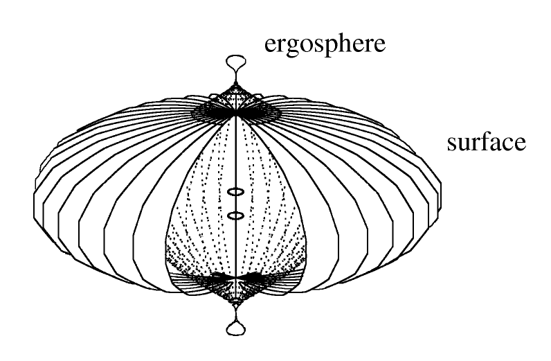
Figure 18: Ring currents as sources of the exterior fields

It is clear that a vacuum solution is not able to describe the interior of the star. For each EOS the parameters have to be adjusted to match both regions. Therefore this solution cannot claim to be global and the presence of (naked) singularities which are always inside the stellar surface is irrelevant for astrophysics. However they help to interprete the exterior field as a space-time created by a configuration with two ring currents (Fig. 18). These mass- and angular momentum currents arise as singularities in the curvature tensor. Coupled by the Einstein equations to the energy-momentum-tensor of the electromagnetic fields these sources should also appear in the electric and magnetic field-distributions. Because of charge neutrality the ring currents must have different rotation directions and therefore create also weak electromagnetic quadrupole fields. As discussed in section 7 it seems to be common that the ergoregion is not completely enclosed by the stellar surface. The fact that it leak from the interior of the star only in the polar regions could have very interesting consequences for the acceleration of particles and propagation of light.

References

• [1993] Aguirregabaria, J. M., Chamorro, A., Manko, V. S., Sibgatullin, N. R., 1993, Phys. Rev. D, 48, 622
• [2002] Ansorg, M., Kleinwächter, A., Meinel, R., 2002, A & A, 381, L49
• [1994] Cook, G. B., Shapiro, S. L., Teukolsky, S. A., 1994, ApJ, 424, 823
• [1968] Ernst, F. J., 1968, Phys. Rev., 168, 1415
• [2001] Glendenning, N. K., Weber, F., 2001, ApJ, 559, L119
• [1989] Komatsu, H., Eriguchi, Y., Hachisu, I., 1989, MNRAS, 237, 355
• [1994] Manko, V. S., Martin, J., Ruiz, E., Sibgatullin, N. R., Zaripov, M. N., 1994, Phys. Rev. D, 49, 5144
• [1999] Manko, O. V., Manko, V. S., Sanabria-G$\acute{\textrm{o}}$mez, J. D., 1999, Gen. Rel. Grav., 31, 1539
• [2000] Manko, V. S., Sanabria-G$\acute{\textrm{o}}$mez, J. D., Manko, O. V., 2000, Phys. Rev. D, 62, 044048
• [1996] Miller, M. C., Lamb, F. K., 1996, ApJ, 470, 1033
• [1980] Paczy$\acute{\textrm{n}}$ski, B., Wiita, P. J., 1980, A & A, 88, 23
• [1953] Papapetrou, A., 1953, Ann. Phys., 12, 309
• [1991] Sibgatullin, N. R., Oscillations and Waves in Strong Gravitational and Electromagnetic Fields, Nauka, Moskau, 1984; English translation: Springer, Berlin, 1991
• [1998] Sibgatullin, N. R., Sunyaev, R. A., 1998, Astron. Let., 24, 894
• [2000] Sibgatullin, N. R., Sunyaev, R. A., 2000, Astron. Let., 26, 699
• [1986] Thorne, K. S., Price, R. H., MacDonald, D. A., Black Holes: The Membrane Paradim, Yale University Press, New Haven, 1986
• [1999] Thorsett, S. E., Chakrabarty, D., 1999, ApJ, 512, 288