Generation of Compressible Modes in MHD Turbulence

Abstract

Astrophysical turbulence is magnetohydrodynamic (MHD) in its nature. We discuss fundamental properties of MHD turbulence. In particular, we discuss the generation of compressible MHD waves by Alfvenic turbulence and show that this process is inefficient. This allows us to study the evolution of different types of MHD perturbations separately. We describe how to separate MHD fluctuations into 3 distinct families - Alfven, slow, and fast modes. We find that the degree of suppression of slow and fast modes production by Alfvenic turbulence depends on the strength of the mean field. We show that Alfven modes in compressible regime exhibit scalings and anisotropy similar to those in incompressible regime. Slow modes passively mimic Alfven modes. However, fast modes exhibit isotropy and a scaling similar to that of acoustic turbulence both in high and low $\beta$ plasmas. We show that our findings entail important consequences for theories of star formation, cosmic ray propagation, dynamics of dust, and gamma ray bursts. We anticipate many more applications of the new insight to MHD turbulence and expect more revisions of the existing paradigms of astrophysical processes as the field matures.

1 Introduction

Astrophysics has been providing the major incentive for MHD studies. High conductivity of astrophysical fluids makes magnetic fields “frozen in”, and they affect fluid motions. The coupled motion of magnetic field and conducting fluid is what a researcher has to deal with while studying various astrophysical phenomena from star formation to gamma ray bursts.

Turbulence is ubiquitous in astrophysical fluids and it holds the key to many astrophysical processes (stability of molecular clouds, heating of the interstellar medium, properties of accretion disks, cosmic ray transport etc). Why would we expect astrophysical fluids to be turbulent? A fluid of viscosity $\nu$ gets turbulent when the rate of viscous dissipation, which is $\sim\nu/L^{2}$ at the energy injection scale $L$, is much smaller than the energy transfer rate $\sim V_{L}/L$, where $V_{L}$ is the velocity dispersion at the scale $L$. The ratio of the two rates is the Reynolds number $Re=V_{L}L/\nu$. In general, when $Re$ is larger than $10-100$ the system becomes turbulent. Chaotic structures develop gradually as $Re$ increases, and those with $Re\sim 10^{3}$ are appreciably less chaotic than those with $Re\sim 10^{8}$. Observed features such as star forming clouds are very chaotic with $Re>10^{8}$, which ensures that the fluids are turbulent. The measured statistics of fluctuations ISM ArmRS95 ; StaL01 ; DesDG00 and Solar wind fluctuations LeaSN98 show signatures of the Kolmogorov statistics obtained for incompressible unmagnetized turbulent fluid.

Kolmogorov theory Kol41 provides a scaling law for incompressible non-magnetized hydrodynamic turbulence. This law is true in the statistical sense and it provides a relation between the relative velocity $v_{l}$ of fluid elements and their separation $l$, namely, $v_{l}\sim l^{1/3}$. An equivalent description is to express spectrum $E(k)$ as functions of wave number $k$ ($\sim 1/l$). The two descriptions are related by $kE(k)\sim v_{l}^{2}$. The famous Kolmogorov spectrum is $E(k)\sim k^{-5/3}$. The applications of Kolmogorov theory range from engineering research to meteorology (see MonY75 ) but its astrophysical applications are poorly justified.

Unlike laboratory turbulence astrophysical turbulence is magnetized and highly compressible. Then, why do astrophysical fluids show signatures of Kolmogorov statistics? Let us consider incompressible MHD turbulence first. There have long been understanding that the MHD turbulence is anisotropic (e.g. SheMM83 ). A substantial progress has been achieved recently by Goldreich & Sridhar GolS95 (hereafter GS95) who made a prediction regarding relative motions parallel and perpendicular to magnetic field B for incompressible MHD turbulence. The GS95 model envisages a Kolmogorov spectrum of velocity and the scale-dependent anisotropy (see below). These relations have been confirmed numerically (Cho & Vishniac ChoV00b ; Maron & Goldreich MarG01 ; Cho, Lazarian & Vishniac ChoLV02b , hereafter CLV02b; see also review by Cho, Lazarian, & Vishniac ChoLV02a , hereafter CLV02a); they are in good agreement with observed and inferred astrophysical spectra (see CLV02a). A remarkable fact revealed in CLV02b is that fluid motions perpendicular to B are identical to hydrodynamic motions. This provides an essential physical insight into why in some respects MHD turbulence and hydrodynamic turbulence are similar, while in other respects they are different.

However, in most cases compressibility of turbulence is important. For instance, interstellar medium is highly compressible and star formation requires considering supersonic compressible motions (see reviews VazOP00 ; MacK03 ; ZweHF02 ). It can be shown that assuming that only incompressible turbulence exists in ISM results in grossly erroneous conclusions for cosmic ray transport (see review LazCY03 ). It may be an important question whether the physical pictures in incompressible and compressible turbulence are similar. For instance, Cho, Lazarian & Vishniac ChoLV02c (henceforth CLV02c) reported a new regime of turbulence that takes place in a partially ionized gas. In this regime turbulent energy protrudes to small scales through a magnetic cascade, while the turbulent velocities are suppressed. How will compressibility affect this regime?

Compressible turbulence is an unsolved problem even in the absence of magnetic fields. How feasible is it to strive for obtaining universal scaling relations for compressible media in view of the fact that no such universality exists for compressible hydro turbulence? The difficulty one encounters while studying compressible MHD is that MHD turbulence is in general more complicated than its hydrodynamic counterpart. In compressible regime, 3 different types of motions (Alfven, slow, and fast modes) exist. Alfven modes are incompressible and sometimes called shear Alfven modes. The other two modes are compressible modes (see §3.2). How do those modes interact? Is it reasonable to talk about separate modes in highly non-linear MHD turbulence? These and similar questions dealing with fundamental properties of MHD turbulence we will attempt to answer below.

Thus we must consider a more realistic case of compressible MHD turbulence. Literature on the properties of compressible MHD is very rich (see CLV02a). Back in 80s Higdon Hig84 theoretically studied density fluctuations in the interstellar MHD turbulence. Matthaeus & Brown MatB88 studied nearly incompressible MHD at low Mach number and Zank & Matthaeus ZanM93 extended it. In an important paper Matthaeus et al. MatGO96 numerically explored anisotropy of compressible MHD turbulence. However, those papers do not provide universal scalings of the GS95 type. Some hints about effects of compressibility can be inferred from Goldreich & Sridhar (GS95) seminal paper. A more focused discussion was presented in the Lithwick & Goldreich LitG01 paper which deals with electron density fluctuations in the pressure dominated plasma, i.e. in high $\beta$ regime ($\beta\equiv P_{gas}/P_{mag}\gg 1$). Incompressible regime formally corresponds to $\beta\rightarrow\infty$ and therefore it is natural to expect that for $\beta\gg 1$ the GS95 picture would persist. Lithwick & Goldreich LitG01 also speculated that for low $\beta$ plasmas the GS95 scaling of slow modes may be applicable. A direct study of MHD modes in compressible low $\beta$ plasmas is given in Cho & Lazarian ChoL02a (hereafter CL02), and more general results applicable for a wide range of $\beta$ and Mach numbers are presented in Cho & Lazarian ChoL03a (hereafter CL03).

The generation of slow and fast modes (i.e. MHD version of “sound waves”) has important astrophysical implications. First, in the presence of damping, density and non-Alfvenic magnetic fluctuations are generated only through compressible daughter waves (i.e. slow and fast waves) generated by Alfven turbulence. These fluctuations are important for interstellar physics and cosmic ray physics. Second, if Alfvenic modes produce a copious amount of compressible modes, the whole picture of independent Alfvenic turbulence fails. Therefore, inefficient generation of compressible modes from Alfven turbulence is a necessary condition for independent Alfvenic cascade.

In what follows we review observational data on statistics of turbulence, including the velocity data available through spectral line studies §2. In §3 we describe our technique for decomposing MHD turbulence into Alfven, slow and fast modes. Mode coupling is discussed in §4, while simple theoretical arguments about mode scalings are provided in §5. We describe scalings of velocity fluctuations in §6 and magnetic and density fluctuations in §7. The new regime of turbulence that emerges below the viscous cut-off is briefly discussed in §8. §9 deals with the applicability of our results and with their significance for the theories of star formation, cosmic ray propagation, gamma ray bursts etc. The summary is given in §10.

2 Observational Motivation

Observations as well as space missions provide data on the statistics of astrophysical turbulence. This data suggests that in a wide variety of circumstances astrophysical turbulence exhibits power-law spectra consistent with Kolmogorov picture. It would be very naive to think that, in the presence of dynamically important magnetic fields, the turbulence may really be Kolmogorov, but it is suggestive that, for a wide variety of circumstances, the turbulence should allow pretty simple statistical description. This strongly motivates a quest for simple relations to describe the apparently complex phenomenon.

Direct studies of turbulence have been done mostly for interstellar medium and for the Solar wind. While for the Solar wind in-situ measurements are possible, studies of interstellar turbulence require inverse techniques to interpret the observational data.

Attempts to study interstellar turbulence with statistical tools date as far back as the 1950s Hor51 ; Kam55 ; Mun58 ; WilMF59 and various directions of research achieved various degree of success (see reviews by KapP70 ; Dic85 ; ArmRS95 ; Laz99a ; Laz99b ; LazPE02 ).

2.1 Solar wind

Solar wind (see review GolR95 ) is a magnetized flow of particles (mostly electrons and protons) from the Sun. Studies of the solar wind allow point-wise statistics to be measured directly using spacecrafts. These studies are the closest counterpart of laboratory measurements.

The solar wind flows nearly radially away from the Sun, at up to $\sim$700 km/s. This is much faster than both spacecraft motions and the Alfvén speed. Therefore, the turbulence is “frozen” and the fluctuations at frequency $f$ are directly related to fluctuations at the scale $k$ in the direction of the wind, as $k=2\pi f/v$, where $v$ is the solar wind velocity Hor99 .

The solar wind shows $f^{-5/3}$ scaling on small scales. The turbulence is strongly anisotropic (see KleBB93 ) with the ratio of power in motions perpendicular to the magnetic field to those parallel to the magnetic field being around 30. The intermittency of the solar wind turbulence is very similar to the intermittency observed in hydrodynamic flows HorB97 .

2.2 Electron density statistics in the ISM

Studies of turbulence statistics of ionized media in the interstellar space (see SpaG90 ) have provided information on the statistics of plasma density at scales $10^{8}$-$10^{15}$ cm. This was based on a clear understanding of processes of scintillations and scattering achieved by theorists (see NarG89 ; GooN85 ). A peculiar feature of the measured spectrum (see ArmRS95 ) is the absence of the slope change at the scale at which the viscosity by neutrals becomes important.

Scintillation measurements are the most reliable data in the “big power law” plot in Armstrong et al. ArmRS95 . However there are intrinsic limitations to the scintillations technique due to the limited number of sampling directions, its relevance only to ionized gas at extremely small scales, and the impossibility of getting velocity (the most important!) statistics directly. Therefore with the data one faces the problem of distinguishing actual turbulence from static density structures. Moreover, the scintillation data do not provide the index of turbulence directly, but only show that the data are consistent with Kolmogorov turbulence. Whether the (3D) index can be -4 instead of -11/3 is still a subject of intense debate Hig84 ; NarG89 . In physical terms the former corresponds to the superposition of random shocks rather than eddies.

2.3 Velocity and density statistics from spectral lines

Atoms and molecules in the interstellar space emit radiation at specific wavelengths. A spectral line from atomic hydrogen with $\lambda_{0}$=21 cm is particularly important in astronomy. Astronomers observe intensity of radiation at different wavelengths near $\lambda_{0}$ for different points on the sky, which results in a 3D data cube that consists of two spatial (or, angular) coordinates and one wavelength coordinate (i.e. T=T($\theta_{1}$, $\theta_{2}$, $\lambda-\lambda_{0}$), where T is so-called antenna temperature, which measures radiation energy). Using the Doppler shift formula, we can convert the wavelength dimension to the velocity dimension. Such spectral line data cubes are unique sources of information on interstellar turbulence. Doppler shifts due to supersonic motions contain information on the turbulent velocity field which is otherwise difficult to obtain. Moreover, the statistical samples are extremely rich and not limited to discrete directions. In addition, line emission allows us to study turbulence at large scales, comparable to the scales of star formation and energy injection.

However, the problem of separating velocity and density fluctuations within HI data cubes is far from trivial Laz95 ; Laz99b ; LazP00 ; LazPE02 . The analytical description of the emissivity statistics of channel maps (velocity slices) in Lazarian & Pogosyan LazP00 (see also Laz99b ; LazPE02 for reviews) shows that the relative contribution of the density and velocity fluctuations depends on the thickness of the velocity slice. In particular, the power-law asymptote of the emissivity fluctuations changes when the dispersion of the velocity at the scale under study becomes of the order of the velocity slice thickness (the integrated width of the channel map). These results are the foundation of the Velocity-Channel Analysis (VCA) technique which provides velocity and density statistics using spectral line data cubes. The VCA has been successfully tested using data cubes obtained via compressible magnetohydrodynamic simulations and has been applied to Galactic and Small Magellanic Cloud atomic hydrogen (HI) data LazPV01 ; LazP00 ; StaL01 ; DesDG00 . Furthermore, the inclusion of absorption effects LazP03 has increased the power of this technique. Finally, the VCA can be applied to different species (CO, H_α etc.) which should further increase its utility in the future.

Within the present discussion a number of results obtained with the VCA are important. First of all, the Small Magellanic Cloud (SMC) HI data exhibit a Kolmogorov-type spectrum for velocity and HI density from the smallest resolvable scale of 40 pc to the scale of the SMC itself, i.e. 4 kpc. Similar conclusions can be inferred from the Galactic data Gre93 for scales of dozens of parsecs, although the analysis has not been done systematically. Deshpande et al. DesDG00 studied absorption of HI on small scales toward Cas A and Cygnus A. Within the VCA their results can be interpreted as implying that on scales less than 1 pc the HI velocity is suppressed by ambipolar drag and the spectrum of density fluctuations is shallow $P(k)\sim k^{-2.8}$. Such a spectrum Des00 can account for the small scale structure of HI observed in absorption.

2.4 Magnetic field statistics

Magnetic field statistics are the most poorly constrained aspect of ISM turbulence. The polarization of starlight and of the Far-Infrared Radiation (FIR) from aligned dust grains is affected by the ambient magnetic fields. Assuming that dust grains are always aligned with their longer axes perpendicular to magnetic field (see review Laz00a ), one gets the 2D distribution of the magnetic field directions in the sky. Note that the alignment is a highly non-linear process in terms of the magnetic field and therefore the magnetic field strength is not available.

The statistics of starlight polarization (see FosLP02 ) is rather rich for the Galactic plane and it allows to establish the spectrum $E(K)\sim K^{-1.5}$, where $K$ is a two dimensional wave vector describing the fluctuations over sky patch.

For uniformly sampled turbulence it follows from Lazarian & Shutenkov LazS90 that $E(K)\sim K^{\alpha}$ for $K<K_{0}$ and $K^{-1}$ for $K>K_{0}$, where $K_{0}^{-1}$ is the critical angular size of fluctuations which is proportional to the ratio of the injection energy scale to the size of the turbulent system along the line of sight. For Kolmogorov turbulence $\alpha=-11/3$.

However, the real observations do not uniformly sample turbulence. Many more close stars are present compared to the distant ones. Thus the intermediate slops are expected. Indeed, Cho & Lazarian ChoL02b showed through direct simulations that the slope obtained in FosLP02 is compatible with the underlying Kolmogorov turbulence. At the moment FIR polarimetry does not provide maps that are really suitable to study turbulence statistics. This should change soon when polarimetry becomes possible using the airborne SOFIA observatory. A better understanding of grain alignment (see Laz00a ) is required to interpret the molecular cloud magnetic data where some of the dust is known not to be aligned (see LazGM97 and references therein).

Another way to get magnetic field statistics is to use synchrotron emission. Both polarization and intensity data can be used. The angular correlation of polarization data BacBP01 shows the power-law spectrum $K^{-1.8}$ and we believe that the interpretation of it is similar to that of starlight polarization. Indeed, Faraday depolarization limits the depth of the sampled region. The intensity fluctuations were studied in LazS90 with rather poor initial data and the results were inconclusive. Cho & Lazarian ChoL02b interpreted the fluctuations of synchrotron emissivity GiaBF01 ; GiaBG02 in terms of turbulence with Kolmogorov spectrum.

3 Numerical Approach

3.1 Helmholtz decomposition for hydrodynamic turbulence

To get an insight of the turbulence cascade we have attempted a decomposition of the MHD turbulent flow into Alfven, slow and fast modes (see CL02, CL03). Our numerical method is similar to the technique utilizing the “Helmholtz” decomposition in hydrodynamics.

Our method is different from Lighthill’s theory Lig52 of far field acoustic wave generation from homogeneous turbulence. Literature on the application of Lighthill’s approximation to astrophysical problems is rich. Astrophysical fluids are stratified (by gravity) and/or magnetized. Therefore, Lighthill’s theory requires modifications for astrophysical fluids. Stein Ste67 extended Lighthill’s theory to stratified astrophysical fluids in gravitational field. Subsequent papers (e.g. GolK90 ) further discussed about generation of acoustic waves in (Solar) convection zone. On the other hand, Musielak & Rosner MusR88 constructed a model for weak magnetic field convection zone and Musielak, Rosner, & Ulmschneider MusRU89 discussed about wave generation in an inactive flux tube. Lee Lee93 explored wave generation in sunspots, which are the most strongly magnetized on the surface of the Sun. All these approaches are to calculate far-field acoustic flux.

Moyal Moy51 introduced a method that decomposes velocity field in Fourier space, which is equivalent to Helmholtz’s decomposition of a vector field: ${\bf V}={\bf V}_{s}+{\bf V}_{c}$, where ${\bf V}_{s}$ is divergence-free ($\nabla\cdot{\bf V}_{s}$=0) field and ${\bf V}_{c}$ is curl-free ($\nabla\times{\bf V}_{c}$=0) field. Note that ${\bf V}_{s}$ represents incompressible or solenoidal part and ${\bf V}_{c}$ compressible or dilatational one. In Fourier space, solenodal and dilatational components have simple geometrical meanings: ${\bf V}_{s}$ is the component perpendicular to the wave vector ${\bf k}$ and ${\bf V}_{s}$ parallel to ${\bf k}$.

The first (published) numerical simulations of compressible hydrodynamic turbulence were performed by Feiereisen, et al. FeiRF82 . They studied subsonic (sonic Mach numbers, $M_{s}$, up to 0.32) homogeneous shear flows with $64^{3}$ grid points. Passot & Pouquet PasP87 carried out two-dimensional isotropic homogeneous compressible decaying turbulence with $256^{2}$ grid points. They showed that properties of turbulence at low initial Mach numbers ($M_{s}<0.3$) is significantly different from those of higher Mach number ones. Passot, Pouquet, & Woodward PasPW88 simulated two-dimensional isotropic decaying turbulence with initial Mach numbers up to $4$. They provided conjecture for the three-dimensional case and discussed implications of their work on astrophysical fluids in the interstellar medium. Subsequent simulations KidO90a ; KidO90b ; StaYK90 ; SarEH91 ; LeeLM91 addressed various issues of compressible turbulence. Recent high resolution three-dimensional simulations include Porter, Pouquet, & Woodward PorPW92 , Porter, Woodward, & Pouquet PorWP98 , and Porter, Pouquet, & Woodward PorPW02 .

The energy spectra of compressible hydrodynamic turbulence are still uncertain. For spectrum of solenoidal components, a Kolmogorov-type dimensional analysis leads to

$$E_{solenoidal}(k)\propto k^{-5/3}(kL)^{\alpha M_{s}^{2}}$$ (1)

(KadP73 ; see also PasPW88 ). However, Moiseev et al. MoiPT81 obtained slightly different results

$$E_{solenoidal}(k)\propto k^{-5/3}(kL)^{\frac{-2M_{s}^{2}}{3(3-M_{s}^{2})}}.$$ (2)

When, $M_{s}\rightarrow 0$, both results give Kolmogorov spectrum.

The energy spectrum of compressible components is more uncertain. For example, Zakharov & Sagdeev ZakS70 derived scalings for compressible modes:

$$E_{rad}(k)\propto k^{-3/2},$$ (3)

where the subscript rad denotes compressible components (i.e. radial components in Fourier space). On the other hand, Bataille & Zhou BatZ99 and Bertoglio, Bataille, & Marion BerBM01 obtained that the spectral index (slope) is a function of Mach number, $M_{s}$. When, Mach number is of order unity, their results give a Kolmogorov spectrum. Recent numerical simulations PorWP98 with up to $1024^{3}$ grid points show Kolmogorov’s $k^{-5/3}$ spectra both for $E_{solenoidal}(k)$ and $E_{rad}(k)$.

The generation of compressible components from incompressible initial turbulence is also an unresolved issue. Closure calculation by Bataille & Zhou BatZ99 and Bertoglio et al. BerBM01 predicts that $\chi\equiv\langle V_{rad}^{2}\rangle/\langle V_{solenoidal}^{2}\rangle\sim M_{s}^{2}$. Numerical calculations of decaying turbulence with initial Mach number of order unity PorPW92 ; PorPW02 show that $\chi\sim 0.1$.

3.2 MHD mode decomposition

Three types of waves exist (Alfven, slow and fast) in compressible magnetized plasma. In this section, we describe how to separate different MHD modes.

In the presence of magnetic field ${\bf B}$, the momentum equation has an additional term, $(\nabla\times{\bf B})\times{\bf B}$ (divided by $1/4\pi$). This is the so-called ${\bf J}\times{\bf B}$ term, which can be re-written as the sum of the magnetic tension term, ${\bf B}\cdot\nabla{\bf B}$, and magnetic pressure term, $\nabla^{2}{\bf B}$:

$$(\nabla\times{\bf B})\times{\bf B}={\bf B}\cdot\nabla{\bf B}-\nabla^{2}{\bf B}/2.$$ (4)

In addition, when magnetic Reynolds number, $R_{m}=VL/\eta$, where $\eta$ is magnetic diffusivity, is large, magnetic field lines move together with fluid elements, which is sometime called that magnetic fields are frozen-in.

In some sense, the magnetic field lines are like elastic bands moving together with fluid elements in that they have tension. However, they are different from rubber bands in that they are repulsive each other, which is the nature of magnetic pressure.

Because of tension and pressure, the nature of MHD waves is much more complicated than their hydrodynamic counterpart - sound wave. This is because we need to consider 3 different restoring forces - magnetic tension, magnetic pressure, and gas pressure. For Alfven waves, magnetic tension is the only the restoring force (Fig. 1(a)). For slow and fast waves, all 3 restoring forces are important. For Slow waves, magnetic and gas pressure are out of phase and, for fast modes, they are in phase (Fig. 2).

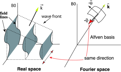
(a)

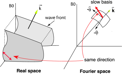
(b)

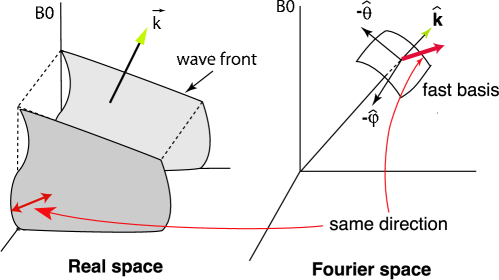
(c)

Figure 1: (a) Alfven wave and its direction of oscillation/displacement. The direction of displacement is perpendicular to both ${\bf B}_{0}$ and ${\bf k}$. Only magnetic tension is the restoring force. (b) Slow wave and its direction of oscillation/displacement. The direction of displacement is between $-\hat{\bf\theta}$ and $\hat{\bf B}_{0}$. (c) Slow wave and its direction of oscillation/displacement. The direction of displacement is between $\hat{\bf k}$ and $\hat{\bf k}_{\perp}$.

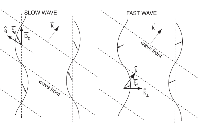
Figure 2: Slow and fast waves in real space (${\bf B}_{0}-{\bf k}$ plane). We show the directions of displacement vectors for a slow wave (left panel) and a fast wave (right panel). Note that $\hat{\xi}_{s}$ lies between $\hat{\theta}$ and $\hat{\bf B}_{0}~{}(=\hat{\bf k}_{\|})$ and $\hat{\xi}_{f}$ between $\hat{\bf k}$ and $\hat{\bf k}_{\perp}$. Again, $\hat{\theta}$ is perpendicular to $\hat{\bf k}$ and parallel to the wave front. Note also that, for the fast wave, for example, density (inferred by the directions of the displacement vectors) becomes higher where field lines are closer, resulting in a strong restoring force, which is why fast waves are faster than slow waves. From CLV02a.

The slow, fast, and Alfven bases that denote the direction of displacement vectors for each mode are given by

$$\hat{\bf\xi}_{s}\propto(-1+\alpha-\sqrt{D})k_{\|}\hat{\bf k}_{\|}+(1+\alpha-\sqrt{D})k_{\perp}\hat{\bf k}_{\perp},$$ (5)

$$\hat{\bf\xi}_{f}\propto(-1+\alpha+\sqrt{D})k_{\|}\hat{\bf k}_{\|}+(1+\alpha+\sqrt{D})k_{\perp}\hat{\bf k}_{\perp},$$ (6)

$$\hat{\bf\xi}_{A}\propto\hat{\bf\varphi}\propto\hat{\bf k}_{\perp}\times\hat{\bf k}_{\|},$$ (7)

where $D=(1+\alpha)^{2}-4\alpha\cos\theta$, $\alpha=a^{2}/V_{A}^{2}=\beta(\gamma/2)$, $\theta$ is the angle between ${\bf k}$ and ${\bf B}_{0}$, and $\hat{\bf\varphi}$ is the azimuthal basis in the spherical polar coordinate system (see Appendix). These are equivalent to the expression in CL02:

$$\hat{\bf\xi}_{s} \propto k_{\|}\hat{\bf k}_{\|}+\frac{1-\sqrt{D}-{\beta}/2}{1+\sqrt{D}+{\beta}/2}\left[\frac{k_{\|}}{k_{\perp}}\right]^{2}k_{\perp}\hat{\bf k}_{\perp},$$ (8)

$$\hat{\bf\xi}_{f} \propto \frac{1-\sqrt{D}+{\beta}/2}{1+\sqrt{D}-{\beta}/2}\left[\frac{k_{\perp}}{k_{\|}}\right]^{2}k_{\|}\hat{\bf k}_{\|}+k_{\perp}\hat{\bf k}_{\perp}.$$ (9)

(Note that $\gamma=1$ for isothermal case.)

We can obtain slow and fast velocity by projecting velocity Fourier component ${\bf v}_{\bf k}$ into $\hat{\bf\xi}_{s}$ and $\hat{\bf\xi}_{f}$, respectively. In Appendix, we also discuss how to separate slow and fast magnetic modes. We obtain energy spectra using this projection method.

3.3 Numerical method

We use a hybrid essentially non-oscillatory (ENO) scheme to solve the ideal isothermal MHD equations. When variables are sufficiently smooth, we use the 3rd-order Weighted ENO scheme JiaW99 without characteristic mode decomposition. When the opposite is true, we use the 3rd-order Convex ENO scheme LiuO98 . Combined with a three-stage Runge-Kutta method for time integration, our scheme gives third order accuracy in space and time. We solve the ideal MHD equations in a periodic box:

$${\partial\rho}/{\partial t}+\nabla\cdot(\rho{\bf v})=0,$$ (10)

$${\partial{\bf v}}/{\partial t}+{\bf v}\cdot\nabla{\bf v}+\rho^{-1}\nabla(a^{2}\rho)-(\nabla\times{\bf B})\times{\bf B}/4\pi\rho={\bf f},$$ (11)

$${\partial{\bf B}}/{\partial t}-\nabla\times({\bf v}\times{\bf B})=0,$$ (12)

with $\nabla\cdot{\bf B}=0$ and an isothermal equation of state. Here $\bf{f}$ is a random large-scale driving force, $\rho$ is density, ${\bf v}$ is the velocity, and ${\bf B}$ is magnetic field. The rms velocity $\delta V$ is maintained to be unity, so that ${\bf v}$ can be viewed as the velocity measured in units of the r.m.s. velocity of the system and ${\bf B}/\sqrt{4\pi\rho}$ as the Alfvén speed in the same units. The time $t$ is in units of the large eddy turnover time ($\sim L/\delta V$) and the length in units of $L$, the scale of the energy injection. The magnetic field consists of the uniform background field and a fluctuating field: ${\bf B}={\bf B}_{0}+{\bf b}$.

For mode coupling studies (Fig. 4), we do not drive turbulence. For scaling studies, we drive turbulence solenoidally in Fourier space and use $216^{3}$ points and $\rho_{0}=1$. The average rms velocity in statistically stationary state is $\delta V\sim 0.7$.

For our calculations we assume that $B_{0}/\sqrt{4\pi\rho}\sim\delta B/\sqrt{4\pi\rho}\sim\delta V$. In this case, the sound speed is the controlling parameter and basically two regimes can exist: supersonic and subsonic. Note that supersonic means low-beta and subsonic means high-beta. When supersonic, we consider mildly supersonic (or, mildly low-$\beta$) and highly supersonic (or, very low-$\beta$).

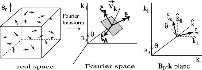
Figure 3: Separation method. We separate Alfven, slow, and fast modes in Fourier space by projecting the velocity Fourier component ${\bf v_{k}}$ onto bases ${\bf\xi}_{A}$, ${\bf\xi}_{s}$, and ${\bf\xi}_{f}$, respectively. Note that ${\bf\xi}_{A}=-\hat{\bf\varphi}$. Slow basis ${\bf\xi}_{s}$ and fast basis ${\bf\xi}_{f}$ lie in the plane defined by ${\bf B}_{0}$ and ${\bf k}$. Slow basis ${\bf\xi}_{s}$ lies between $-\hat{\bf\theta}$ and $\hat{\bf k}_{\|}$. Fast basis ${\bf\xi}_{f}$ lies between $\hat{\bf k}$ and $\hat{\bf k}_{\perp}$. From CL03.

4 Mode Coupling: Theory and Simulations

As mentioned above, the coupling of compressible and incompressible modes is crucial. If Alfvenic modes produce a copious amount of compressible modes, the whole picture of independent Alfvenic turbulence fails.

The generation of compressible motions (i.e. radial components in Fourier space) from Alfvenic turbulence is a measure of mode coupling. How much energy in compressible motions is drained from Alfvenic cascade? According to the closure calculations (BerBM01 ; see also ZanM93 ), the energy in compressible modes in hydrodynamic turbulence scales as $\sim M_{s}^{2}$ if $M_{s}<1$. We may conjecture that this relation can be extended to MHD turbulence if, instead of $M_{s}^{2}$, we use $\sim(\delta V)_{A}^{2}/(a^{2}+V_{A}^{2})$. (Hereinafter, we define $V_{A}\equiv B_{0}/\sqrt{4\pi\rho}$.) However, as the Alfven modes are anisotropic, this formula may require an additional factor. The compressible modes are generated inside so-called Goldreich-Sridhar cone, which takes up $\sim(\delta V)_{A}/V_{A}$ of the wave vector space. The ratio of compressible to Alfvenic energy inside this cone is the ratio given above. If the generated fast modes become isotropic (see below), the diffusion or, “isotropization” of fast wave energy in the wave vector space increase their energy by a factor of $\sim V_{A}/(\delta V)_{A}$. This results in

$$\frac{(\delta V)_{rad}^{2}}{(\delta V)_{A}^{2}}\sim\left[\frac{V_{A}^{2}+a^{2}}{(\delta V)^{2}_{A}}\frac{(\delta V)_{A}}{V_{A}}\right]^{-1},$$ (13)

where $(\delta V)_{rad}^{2}$ and $(\delta V)_{A}^{2}$ are energy of compressible and Alfven modes, respectively. Eq. (13) suggests that the drain of energy from Alfvenic cascade is marginal when the amplitudes of perturbations are weak, i.e. $(\delta V)_{A}\ll V_{A}$.

Fig. 4(a) shows that generation of slow and fast modes (the dotted line) from Alfven modes (the solid line) is marginal. The result shown in the figure is for $M_{s}=1.6$ at $t=0$. We repeated similar simulation for different Mach numbers and plasma $\beta$’s and measured the ratios of energy in compressible modes to that in Alfven modes. The results are shown in Fig. 4(c) and (d). Fig. 4(c) suggest that the generation of compressible motions follows equation (13). Fast modes also follow a similar scaling, although the scatter is a bit larger. Fig. 4(e) demonstrates that fast modes are initially generated anisotropically, which supports our theoretical consideration above. Fast modes becomes isotropic later (Fig. 4(f)). Fig. 4(d) shows that generation of slow modes follows $(\delta V)_{s}^{2}/(\delta V)_{A}^{2}\propto(\delta V)_{A}/V_{A}$ for low $\beta$ cases (pluses in the figure). But, the scaling is not clear for high $\beta$ cases (diamonds in the figure).

Fig. 4(b) shows that dynamics of Alfven modes is not affected by slow modes. The solid line in the figure is the energy in Alfven modes when we start the decay simulation with Alfven modes only. The dotted line is the Alfven energy when we start the simulation with all modes. This result confirms that Alfven modes cascade is almost independent of slow and fast modes. In this sense, coupling between Alfven and other modes is weak.

(a)	(b)
(c)	(d)
(e)	(f)

Figure 4: Generation of compressible MHD modes. (a) When Alfvenic turbulence decays, generation of slow and fast modes is marginal. $144^{3}$. Initially, $\beta$ (ratio of gas to magnetic pressure, $P_{g}/P_{mag}$) $=0.2$ and $M_{s}$ (sonic Mach number) $\sim 1.6$. (b) Comparison of decay rates. Decay of Alfven modes is not much affected by other (slow and fast) modes. We use $144^{3}$ grid points. Initially, $\beta=0.2$ and $M_{s}\sim 1.6$ for the solid line and $M_{s}\sim 2.3$ for the dotted line. (c) Square of the r.m.s. velocity of the compressible modes. We use $144^{3}$ grid points. Only Alfven modes are allowed as the initial condition. “Pluses” are for low $\beta$ cases ($0.02\leq\beta\leq 0.4$). “Diamonds” are for high $\beta$ cases ($1\leq\beta\leq 20$). Fast modes follow a similar scaling. (d) Square of the r.m.s. velocity of the slow modes. See (c) for explanation. (e) Generation of fast modes. Snapshot is taken at t=0.06 from a simulation (with $144^{3}$ grid points) that started off with Alfven modes only. Initially, $\beta=0.2$ and $M_{s}$ (sonic Mach number) $\sim 1.6$. (f) Generation of fast modes. Snapshot is taken at t$\sim$2. See (e) for explanation.

5 Quest for Scaling Relations

5.1 Scaling of incompressible MHD turbulence

As mentioned in §1, Goldreich & Sridhar (GS95) made a prediction regarding relative motions parallel and perpendicular to magnetic field B for incompressible MHD turbulence. Here, we reconstruct GS95 model from different perspectives.

An important observation that leads to understanding of the GS95 scaling is that magnetic field cannot prevent mixing motions of magnetic field lines if the motions are perpendicular to magnetic field. Those motions will cause, however, waves that will propagate along magnetic field lines. If that is the case, the time scale of wave-like motion, i.e. $\sim l_{\|}/V_{A}$, where $l_{\|}$ is the characteristic size of the perturbation and $V_{A}$ is the local Alfven speed, will be equal to the hydrodynamic time-scale, $l_{\perp}/v_{l}$. The mixing motions are hydrodynamic-like and therefore obey Kolmogorov scaling $v_{l}\propto l_{\perp}^{1/3}$. Equating the two relations above, we obtain a critically balance condition

$$l_{\|}/V_{A}\sim l_{\perp}/v_{k}\mbox{ ~{}(or $k_{\|}V_{A}\sim k_{\perp}v_{k}$).}$$ (14)

If conservation of energy in the turbulent cascade applies locally in phase space then the energy cascade rate ($v_{l}^{2}/t_{cas}$) is constant): $(v_{l}^{2})/(l_{\perp}/v_{l})=\mbox{constant.}$ Combining this with the critical balance condition we obtain

$$l_{\|}\propto l_{\perp}^{2/3}$$ (15)

(or $k_{\|}\propto k_{\perp}^{2/3}$ in terms of wavevectors) and and a Kolmogorov-like spectrum for perpendicular motions

$$v_{l}\propto l_{\perp}^{1/3},\mbox{~{}~{}or,~{}}E(k)\propto k_{\perp}^{-5/3},$$ (16)

which is not surprising since perpendicular motions are hydrodynamic. If we interpret $l_{\|}$ as the eddy size in the direction of the local field and $l_{\perp}$ as that in the perpendicular direction, the relation in equation (15) implies that smaller eddies are more elongated (see Fig. 5 for illustration of scale-dependent anisotropy).

Using Matthaeus et al. MatOG98 result, we can re-derive GS95 model. Matthaeus et al. MatOG98 showed that the anisotropy of low frequency MHD turbulence scales linearly with the ratio of perturbed and total magnetic field strength $b/B$ ($=b/(b^{2}+B_{0}^{2})^{1/2}$). This scaling relation has simple geometric meaning: perpendicular size of a large scale eddy is similar to its parallel size times $b/B$, which is is determined by magnetic field line wandering. Although their analysis was based on comparing the strength of a uniform background field and the magnetic perturbations on all scales, we can reinterpret this result by assuming that the strength of random magnetic field at a scale $l$ is $b_{l}$, and that the background field is the sum of all contributions from larger scales. Then Matthaeus et al.’s result becomes a prediction that the anisotropy ($k_{\parallel}/k_{\perp}$) is proportional to ($b_{l}/B$). We can take the total magnetic field strength $B\sim$ constant as long as the background field is stronger than the perturbations on all scales. Since $b_{l}\sim(kE(k))^{1/2}\sim k_{\perp}^{-1/3}$, we obtain an anisotropy ($k_{\parallel}/k_{\perp}$) proportional to $k_{\perp}^{-1/3}$, and $k_{\parallel}\propto k_{\perp}^{2/3}$. In this interpretation, smaller eddies are more elongated because they have a smaller $b_{l}/B$ ratio.

5.2 Compressible scalings: theoretical considerations

In §4, we showed that Alfven modes are independent of other modes. Therefore, we expect GS95 scalings for Alfven modes even for supersonic turbulence.

When Alfven cascade evolves on its own, it is natural to assume that slow modes passively follow the Alfven cascade and exhibit the same scaling. Indeed, slow modes in high $\beta$ plasmas are similar to the pseudo-Alfven modes in incompressible regime (see GS95; LitG01 ). The latter modes do follow the GS95 scaling. In low $\beta$ plasmas, motions of slow modes are density perturbations propagating with the sound velocity $a$ parallel to the mean magnetic field (see equation (81)). In magnetically dominated environments ($\beta\ll 1$), $a\ll V_{A}$ and the gaseous perturbations are essentially static. Therefore the magnetic field mixing motions are expected to mix density perturbations as if they were passive scalar. It is known that the passive scalar shows the same scaling as the velocity field of the inducing turbulent motions. Thus the slow waves are expected to demonstrate GS95 scalings (see CL02).

The fast waves in low $\beta$ regime propagate at $V_{A}$ irrespectively of the magnetic field direction. In high $\beta$ regime, the properties of fast modes are similar, but the propagation speed is the sound speed $a$. Thus the mixing motions induced by Alfven waves should affect the fast wave cascade only marginally. The latter cascade is expected to be analogous to the acoustic wave cascade and be isotropic.

6 Velocity scaling

6.1 Illustration of eddy structures

Fig. 5 and Fig. 6 show the shapes of eddies of different sizes. For Alfven mode eddies (Fig. 5), left 3 panels show an increased anisotropy as we move from the top (large eddies) to the bottom (small eddies). The horizontal axes of the left panels are parallel to ${\bf B_{0}}$. Structures in the perpendicular plane (right panels) do not show a systematic elongation. However, Fig. 6 shows that velocity of fast modes exhibit isotropy. Data are from a simulation with $216^{3}$ grid points, $M_{s}=2.3$, and $\beta=0.2$.

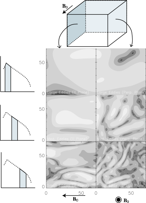
Figure 5: Anisotropy as a function of scale. Alfven mode velocity show scale-dependent anisotropy. Lighter tones are for larger $|{\bf v}|$. Only part of the data cube is shown. Magnetic field show similar behaviors. Large scale eddies are obtained from the Fourier components with $1\leq k<3$. Medium scale eddies are obtained from the Fourier components with $3\leq k<9$. Small scale eddies are obtained from the Fourier components with $9\leq k<27$.

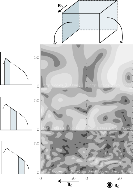
Figure 6: Fast mode velocity show isotropy. Only part of the data cube is shown. Magnetic field show similar behaviors.

6.2 Alfven modes in compressible MHD

If Alfven cascade evolves on its own, it is natural to assume that slow modes exhibit the GS95 scaling. Indeed, slow modes in pressure dominated environment (high $\beta$ plasmas) are similar to the pseudo-Alfven modes in incompressible regime (see GS95; LitG01 ). The latter modes do follow the GS95 scaling. In magnetically dominated environments (low $\beta$ plasmas), slow modes are density perturbations propagating with the sound velocity $a$ parallel to the mean magnetic field (see equation (81)). Those perturbations are essentially static for $a\ll V_{A}$. Therefore Alfvenic turbulence is expected to mix density perturbations as if they were passive scalar. This also induces GS95 spectrum.

Fig. 7(a), (c), and (e) show that the spectra of Alfvén waves follow a Kolmogorov spectrum:

$$\mbox{\it Spectrum of Alfv\'{e}n Waves:~{}~{}~{}}E^{A}(k)\propto k_{\perp}^{-5/3},$$ (17)

regardless of plasma $\beta$ or sonic Mach number $M_{s}$.

In Fig. 7(b), (d), and (f), we plot contours of equal second-order structure function for velocity ($SF_{2}({\bf r})=<|{\bf v}({\bf x}+{\bf r})-{\bf v}({\bf x})|^{2}>_{avg.~{}over~{}{\bf x}}$) obtained in local coordinate systems in which the parallel axis is aligned with the local mean field (see ChoV00b ;MarG01 ; CLV02b). The $SF_{2}$ along the axis perpendicular to the local mean magnetic field follows a scaling compatible with $r^{2/3}$. The $SF_{2}$ along the axis parallel to the local mean field follows steeper $r^{1}$ scaling. The results are compatible with the GS95 model,

$$\mbox{\it Anisotropy of Alfv\'{e}n Waves:~{}~{}~{}}r_{\|}\propto r_{\perp}^{2/3},\mbox{~{}or~{}}k_{\|}\propto k_{\perp}^{2/3},$$ (18)

where $r_{\|}$ and $r_{\perp}$ are the semi-major axis and semi-minor axis of eddies, respectively ChoV00b . When we interpret that contours represent eddy shapes, the above scaling means that smaller contours are more elongated.

(a)	(b)
(c)	(d)
(e)	(f)

Figure 7: Alfven modes. (a)&(b): $M_{s}\sim 0.35$ ($\beta=4$). (c)&(d): $M_{s}\sim 2.3$ ($\beta=0.2$). (e)&(f): $M_{s}\sim 7$ ($\beta=0.02$). Spectra are compatible with Kolmogorov. Contours (or, eddy shapes) show scale-dependent anisotropy: smaller eddies are more elongated. Overall, the scalings are consistent with Goldreich & Sridhar scalings.

6.3 Slow modes in compressible MHD

The incompressible limit of slow waves is pseudo-Alfvén waves. Goldreich & Sridhar GolS97 argued that the pseudo-Alfvén waves are slaved to the shear-Alfvén (i.e. ordinary Alfvén) waves, which means that pseudo-Alfvén modes do not cascade energy for themselves. Lithwick & Goldreich LitG01 made similar theoretical arguments for high $\beta$ plasmas and conjectured similar behaviors of slow modes in low $\beta$ plasmas. We confirmed that similar arguments are also applicable to slow waves in low $\beta$ plasmas (CL02). Indeed, energy spectra in Fig. 8(a) and (c) are consistent with:

$$\mbox{\it Spectrum of Slow Modes:~{}~{}~{}}E^{s}(k)\propto k_{\perp}^{-5/3}.$$ (19)

However, the kinetic energy spectrum for slow modes in Fig. 8(e) does not show the Kolmogorov slope. The slope is close to $-2$, which is suggestive of shock formation. At this moment, it is not clear whether or not the $-2$ slope is the true slope. In other words, the observed $-2$ slope might be due to the limited numerical resolution. Runs with higher numerical resolution should give the definite answer.

In Fig. 8(b), (d), and (f), contours of equal second-order velocity structure function ($SF_{2}$), representing eddy shapes, show scale-dependent anisotropy: smaller eddies are more elongated. The results are compatible with the GS95 model

$$\mbox{\it Anisotropy of Slow Modes:~{}~{}~{}}k_{\|}\propto k_{\perp}^{2/3},\mbox{~{}or~{}}r_{\|}\propto r_{\perp}^{2/3},$$ (20)

where $r_{\|}$ and $r_{\perp}$ are the semi-major axis and semi-minor axis of eddies, respectively.

(a)	(b)
(c)	(d)
(e)	(f)

Figure 8: Slow modes. (a)&(b): $M_{s}\sim 0.35$ ($\beta=4$). (c)&(d): $M_{s}\sim 2.3$ ($\beta=0.2$). (e)&(f): $M_{s}\sim 7$ ($\beta=0.02$). In (a) and (c), spectra are compatible with Kolmogorov. In (e), spectra is uncertain. Contours (or, eddy shapes) show scale-dependent anisotropy: smaller eddies are more elongated. Overall, the scalings are consistent with Goldreich & Sridhar scalings (except spectra in (e)).

6.4 Fast modes in compressible MHD

Fig. 9(b), (d), and (f) show fast modes are isotropic. The resonance conditions for the interacting fast waves are $\omega_{1}+\omega_{2}=\omega_{3}\mbox{~{}~{}and~{}~{}}{\bf k}_{1}+{\bf k}_{2}={\bf k}_{3}.$ Since $\omega\propto k$ for the fast modes, the resonance conditions can be met only when all three ${\bf k}$ vectors are collinear. This means that the direction of energy cascade is radial in Fourier space. This is very similar to acoustic turbulence, turbulence caused by interacting sound waves Zak67 ; ZakS70 ; LvoLP00 . Zakharov & Sagdeev ZakS70 found $E(k)\propto k^{-3/2}$. However, there is debate about the exact scaling of acoustic turbulence. Here we cautiously claim that our numerical results are compatible with the Zakharov & Sagdeev scaling:

$$\mbox{\it Spectrum of Fast Modes:~{}~{}~{}}E^{f}(k)\sim k^{-3/2}.$$ (21)

The eddies are isotropic (see also Fig. 6).

(a)	(b)
(c)	(d)
(e)	(f)

Figure 9: Fast modes. (a)&(b): $M_{s}\sim 0.35$ ($\beta=4$). (c)&(d): $M_{s}\sim 2.3$ ($\beta=0.2$). (e)&(f): $M_{s}\sim 7$ ($\beta=0.02$). Spectra are compatible with either $k^{-3/2}$ or Kolmogorov. Contours (or, eddy shapes) show isotropy. Overall, the scalings are consistent with those of acoustic turbulence.

7 Magnetic Field and Density Scalings

We expect that isotropy/anisotropy of magnetic field is similar to that of velocity (see CL03). However, anisotropy of density shows different behavior. Density shows anisotropy for the high $\beta$ case. But, for low $\beta$ cases, density shows more or less isotropic structures. We suspect that shock formation is responsible for isotropization of density.

To estimate the r.m.s. fluctuations, we use the following linearized continuity and induction equations:

$$|\rho_{k}| = (\rho_{0}v_{k}/c)|\hat{\bf k}\cdot\hat{\bf\xi}|,$$ (22)

$$|b_{k}| = (B_{0}v_{k}/c)|\hat{\bf B}_{0}\times\hat{\bf\xi}|,$$ (23)

where $c$ denotes velocity of slow or fast waves (equation (72)). From this, we obtain the r.m.s. fluctuations

$$(\delta\rho/\rho_{0})_{s} = (\delta V)_{s}\langle|\hat{\bf k}\cdot\hat{\bf\xi}_{s}/c_{s}|\rangle,$$ (24)

$$(\delta\rho/\rho_{0})_{f} = (\delta V)_{f}\langle|\hat{\bf k}\cdot\hat{\bf\xi}_{f}/c_{f}|\rangle,$$ (25)

$$(\delta B/B_{0})_{s} = (\delta V)_{s}\langle|\hat{\bf B}_{0}\times\hat{\bf\xi}_{s}/c_{s}|\rangle,$$ (26)

$$(\delta B/B_{0})_{f} = (\delta V)_{f}\langle|\hat{\bf B}_{0}\times\hat{\bf\xi}_{f}/c_{f}|\rangle,$$ (27)

where angled brackets denote a proper Fourier space average. Generation of slow and fast modes velocity ($(\delta V)_{s}$ and $(\delta V)_{f}$) depends on driving force. Therefore, we may simply assume that

$$(\delta V)_{A}\sim(\delta V)_{s}\sim(\delta V)_{f},$$ (28)

where we ignore constants of order unity. However, when we consider mostly incompressible driving, the generation fast modes may follow equation (13). In this case, the amplitude of fast mode velocity is reduced by a factor of $\left[\frac{V_{A}^{2}+a^{2}}{(\delta V)^{2}_{A}}\frac{(\delta V)_{A}}{V_{A}}\right]^{-1/2}$:

$$(\delta V)_{A}\sim(\delta V)_{s}\sim\left[\frac{V_{A}^{2}+a^{2}}{(\delta V)^{2}_{A}}\frac{(\delta V)_{A}}{V_{A}}\right]^{1/2}(\delta V)_{f}.$$ (29)

When we assume $(\delta V)_{A}\sim B_{0}$, equation (29) reduces to equation (28) in low $\beta$ plasmas.

7.1 Low-$\beta$ case

In this limit, $c_{s}\sim a\cos\theta$ and $c_{f}\sim V_{A}$. Using equations (81) and (82), we obtain

$$(\delta\rho/\rho_{0})_{s} \sim (\delta V)_{s}\langle|\cos\theta/c_{s}|\rangle\sim(\delta V)_{s}/a,$$ (30)

$$(\delta\rho/\rho_{0})_{f} = (\delta V)_{f}\langle|\sin\theta/c_{f}|\rangle\sim(\delta V)_{f}/V_{A},$$ (31)

$$(\delta B/B_{0})_{s} = (\delta V)_{s}\langle|\alpha\cos\theta\sin\theta/c_{s}|\rangle\sim\alpha(\delta V)_{s}/a,$$ (32)

$$(\delta B/B_{0})_{f} = (\delta V)_{f}\langle|1/c_{f}|\rangle\sim(\delta V)_{f}/V_{A},$$ (33)

where we ignore $\cos\theta$’s or $\sin\theta$’s.

When we assume $(\delta V)_{A}\sim(\delta V)_{s}\sim(\delta V)_{f}\sim B_{0}$, we get

$$(\delta\rho/\rho_{0})_{s} \sim M_{s},$$ (34)

$$(\delta\rho/\rho_{0})_{f} = \sqrt{\beta}M_{s},$$ (35)

$$(\delta B/B_{0})_{s} = \beta M_{s},$$ (36)

$$(\delta B/B_{0})_{f} = \sqrt{\beta}M_{s}$$ (37)

Therefore, in low $\beta$ plasmas, slow modes give rise to most of density fluctuations (CL02). On the other hand, magnetic fluctuation by slow modes is smaller than that by fast modes by a factor of $\sqrt{\beta}$.

7.2 High-$\beta$ case

In this limit, $c_{s}\sim V_{A}\cos\theta$ and $c_{f}\sim a$. Using equations (83) and (84), we obtain

$$(\delta\rho/\rho_{0})_{s} \sim (\delta V)_{s}\langle|\cos\theta\sin\theta/(\alpha c_{s})|\rangle$$ (38)

$$\sim (V_{A}/a)(\delta V)_{s}/a,$$ (39)

$$(\delta\rho/\rho_{0})_{f} = (\delta V)_{f}\langle|1/c_{f}|\rangle\sim(\delta V)_{f}/a,$$ (40)

$$(\delta B/B_{0})_{s} = (\delta V)_{s}\langle|\cos\theta/c_{s}|\rangle\sim(\delta V)_{s}/V_{A},$$ (41)

$$(\delta B/B_{0})_{f} = (\delta V)_{f}\langle|\sin\theta/c_{f}|\rangle\sim(\delta V)_{f}/a,$$ (42)

where we ignore $\cos\theta$’s or $\sin\theta$’s.

Let us just assume that $(\delta V)_{A}\sim(\delta V)_{s}\sim B_{0}\sim M_{s}^{-1}(\delta V)_{f}$ (cf. equation (29)). Then we have

$$(\delta\rho/\rho_{0})_{s} \sim M_{s}/\sqrt{\beta}\sim M_{s}^{2},$$ (43)

$$(\delta\rho/\rho_{0})_{f} \sim M_{s}^{2},$$ (44)

$$(\delta B/B_{0})_{s} = O(1),$$ (45)

$$(\delta B/B_{0})_{f} = M_{s}^{2}.$$ (46)

The density fluctuation associated with slow modes is $\sim M_{s}^{2}$, when $(\delta V)_{s}\sim(\delta V)_{A}\sim V_{A}$. This is consistent with Zank & Matthaeus ZanM93 . The ratio of $(\delta\rho)_{s}$ to $(\delta\rho)_{f}$ is of order unity. Therefore, both slow and fast modes give rise to similar amount of density fluctuations. Note that this argument is of order-of-magnitude in nature. In fact, in our simulations for the high $\beta$ case, the r.m.s. density fluctuation by slow modes is about twice as large as that by fast modes. When we use equation (28), we have a different result: $(\delta\rho)_{s}\sim(V_{A}/a)(\delta\rho)_{f}<(\delta\rho)_{f}$. It is obvious that slow modes dominate magnetic fluctuations: $(\delta B)_{s}>(\delta B)_{f}$ for both equations (28) and (29).

8 Slowly Evolving Fluctuations Below Viscous Cutoff

In hydrodynamic turbulence viscosity sets a minimal scale for motion, with an exponential suppression of motion on smaller scales. Below the viscous cutoff the kinetic energy contained in a wavenumber band is dissipated at that scale, instead of being transferred to smaller scales. This means the end of the hydrodynamic cascade, but in MHD turbulence this is not the end of magnetic structure evolution. For viscosity much larger than resistivity, $\nu\gg\eta$, there will be a broad range of scales where viscosity is important but resistivity is not. On these scales magnetic field structures will be created by the shear from non-damped turbulent motions, which amounts essentially to the shear from the smallest undamped scales. The created magnetic structures would evolve through generating small scale motions. As a result, we expect a power-law tail in the energy distribution, rather than an exponential cutoff. This completely new regime for MHD turbulence was reported in CLV02c. Further research showed that there is a smooth connection between this regime and small scale turbulent dynamo in high Prandtl number fluids (see SchMC02 ).

CLV02c explored this regime numerically with a grid of $384^{3}$ and a physical viscosity for velocity damping. The kinetic Reynolds number was around 100. We achieved a very small magnetic diffusivity by the use of hyper-diffusion. The result is presented in Fig. 10a. A theoretical model for this new regime and its consequences for stochastic reconnection LazV99 can be found in Lazarian, Vishniac, & Cho LazVC03 . It explains the spectrum $E(k)\sim k^{-1}$ as a cascade of magnetic energy to small scales under the influence of shear at the marginally damped scales. The mechanism is based on the solenoidal motions and therefore the compressibility should not alter the physics of this regime of turbulence.

Figure 10: Viscously damped regime (viscosity $>$ magnetic diffusivity). Due to large viscosity, velocity damps after $k\sim 10$. (a) Left: Incompressible case with $384^{3}$ grid points. Magnetic spectra show a shallower slope ($E_{b}(k)\propto k^{-1}$) below the velocity damping scale. From CLV02c. (b) Middle: Compressible case with $216^{3}$ grid points (high $\beta$). Magnetic and density spectra show structures below the velocity damping scale at $k\sim 10$. The spectral slope is poorly defined because it was relatively hard to achieve very small magnetic diffusivity in the compressible run. From CL03. (c) Right: Compressible case with low $\beta$. Density structures are vividly enhanced.

CL03 showed that the new regime of turbulence is also valid for compressible MHD. We use the same physical viscosity as in incompressible case (see CLV02c). We rely on numerical diffusion, which is much smaller than physical viscosity, for magnetic field. The inertial range is much smaller due to numerical reasons, but it is clear that the new regime of MHD turbulence persists. The magnetic fluctuations, however, compress the gas and thus cause fluctuations in density. The amplitude of density perturbations is higher in low $\beta$ plasma (see Fig. 10c). This is a new (although expected) phenomenon compared to our earlier incompressible calculations. These density fluctuations may have important consequences for the small scale structure of the ISM.

9 Discussion

9.1 Range of applicability

One may argue that for the first time ever we have universal scaling relations that describe turbulence over a wide range of plasma $\beta$ and Mach numbers. This remarkable fact entails a lot of astrophysical implications.

Is this consistent with the observational data discussed above?
Yes, we would claim that the observed spectra that are consistent with the Kolmogorov scaling arise naturally. Indeed, Alfven and slow modes exhibit GS95 type scaling. Most of the energy in those modes correspond to perturbations perpendicular to magnetic field. The scaling for the perpendicular motions is Kolmogorov-like, i.e. $E(k)\sim k_{\bot}^{-5/3}$. However, this fact does not imply that it is OK to use Kolmogorov scalings to solve astrophysical problems (see §9.2). It can be a serious mistake to disregard scale-dependent anisotropy of MHD turbulence. Fast modes are isotropic and have a bit different scaling. A more careful analysis of the observational data is necessary to detect the signature of fast modes.

Is super-Alfvenic turbulence different?
In the paper above we considered the cases in which the Alfven speed associated with the mean magnetic field is slightly faster than the r.m.s. fluid velocity. This regime is called “sub-Alfvenic” regime. If initially the turbulent energy is larger than magnetic energy, we are in the regime of so-called “super-Alfvenic” turbulence. In this regime the growth of the magnetic field is expected through so called “turbulent dynamo” (see ChoV00a ; MulB00 ; CLV02a). The magnetic energy at scale $l$ in this regime grows exponentially with the characteristic rate of the eddy turnover time. Thus we expect to reach equipartition between magnetic and kinetic energies at the energy injection scale. At smaller scales the turbulence becomes sub-Alfvenic and our earlier considerations should be applicable. Although the decomposition of MHD turbulence described above does not work for irregular magnetic field characterizing super-Alfvenic turbulence, CL03 results are suggestive that our considerations about Alfven, slow and fast modes are applicable to this regime.

9.2 Compressible MHD turbulence and star formation

How fast does MHD turbulence decay?
This question has fundamental implications for star formation (see McK99 ). Indeed, it was thought originally that magnetic fields would prevent turbulence from fast decay. Later (see MacKB98 ; StoOG98 ; and review VazOP00 ) this was reported not to be true. However, fast decay was erroneously associated with the coupling between compressible and incompressible modes. The idea was that incompressible motions quickly transfer their energy to the compressible modes, which get damped fast by direct dissipation (presumably through shock formation).

Our calculations support the relation in eq. (13). According to it the coupling of Alfven and compressible motions is important only at the energy injection scales where $\delta V_{l}\sim V_{A}$. As the turbulence evolves the perturbations become smaller and the coupling less efficient. Typically for numerical simulations the inertial range is rather small and this could explain why marginal coupling of modes was not noticed.

Our results show that MHD turbulence damping does not depend on whether the fluid is compressible or not. The incompressible motions damp also within one eddy turnover time. This is the consequence of the fact that within the strong turbulence mixing motions perpendicular to magnetic field are hydrodynamic to high order (CLV02b) and the cascade of energy induced by those motions is similar to the hydrodynamic one, i.e. energy cascade happens within an eddy turnover time.

Is the decay always fast for compressible MHD turbulence?
This issue does need further investigation. However, our preliminary answer to this question is “no”. Indeed, incompressible MHD computations (see MarG01 ; CLV02b) show that the rate of turbulence decay depends on the degree of turbulence imbalance, i.e. the difference in the energy fluxes moving in opposite directions. The strongly imbalanced incompressible turbulence was shown to persist longer than its balanced counterpart. This enabled CLV02b to speculate that this may enable energy transfer between clouds and may explain the observed turbulent linewidths of GMCs without evident star formation. Our results above show a marginal coupling of compressible and incompressible modes. This is suggestive that the results obtained in incompressible simulations are applicable to compressible environments if amplitudes of perturbations are not large. The complication arises from the existence of the parametric instability DelVL01 that happens as the density perturbations reflect Alfven waves and grow in amplitude. This instability eventually controls the degree of imbalance that is achievable. However, the growth rate of the instability is substantially slower than the Alfven wave oscillation rate. Therefore, if we take into account that interstellar sources are intermittent not only in space, but also in time, the transport of turbulent energy described in CLV02b may be feasible.

What is the density structure that we expect to see?
First of all, we do not expect to see tight correlation between density and magnetic field. Such sort of correlation is expected in the traditional static picture of the ISM. Introduction of turbulence in the picture of ISM complicates the analysis (see discussion in VazOP00 ; CLV02a). Our results confirm earlier claims (e.g. CLV02a; PasV02 ) that magnetic field - density correlations may be weak. First of all, some magnetic field fluctuations are related to Alfvenic turbulence which does not compress the medium. Second, slow modes in low $\beta$ plasmas are essentially density perturbations that propagate along magnetic field and which marginally perturb magnetic fields.

On the small scales we expect to see structures that anti-correlate with magnetic field and caused by the new regime of turbulence below the ambipolar damping scale. We mentioned above that the simulations in Cho, Lazarian & Vishniac (CLV02c) and theoretical calculations in Lazarian, Vishniac & Cho LazVC03 show that the magnetic field in a newly discovered regime of MHD turbulence can produce a shallow spectrum $E(k)\sim k^{-1}$ spectrum of magnetic fluctuations. Calculations in CL03 suggest that this will translate in the corresponding shallow spectrum of density. For cold neutral medium (CNM; see Draine & Lazarian DraL98 for a list of idealized phases) the spectrum of density fluctuations can protrude from a fraction of parsec to a scale of $\sim 100$ AU (see CL03).

9.3 Astrophysical significance of fast modes

Results of CL02 and CL03 show that the Alfven and slow modes exhibit Goldreich-Sridhar scale-dependent anisotropy. However, it would be very wrong to forget that fast modes are isotropic. It is possible to show that in many instances that difference makes fast modes very important. Consider two examples.

Cosmic Ray Propagation.
The propagation of cosmic rays is mainly determined by their interactions with electromagnetic fluctuations in the interstellar medium. The resonant interaction of cosmic ray particles with MHD turbulence has been repeatedly suggested as the main mechanism for scattering and isotropizing cosmic rays. In these studies, it is usually assumed that the turbulence is isotropic with a Kolmogorov spectrum (e.g. SchM98 ). Yan & Lazarian YanL02 identified fast modes as being responsible for cosmic ray scattering. The scattering by Alfvenic turbulence, which is the default for most of the theoretical constructions, is from 15 to 5 orders smaller than it is usually obtained using Kolmogorov model of Alfvenic turbulence (see Fig. 11).

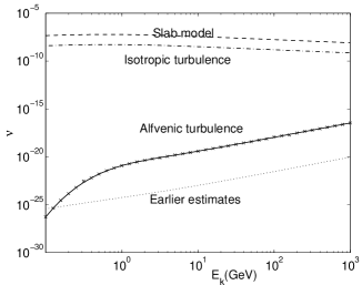
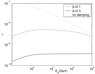
Figure 11: Rate of cosmic ray scattering by Alfvenic (left panel) and fast (right Panel) modes of MHD turbulence. The scattering by Alfvenic modes is negligible, although it is substantially larger than an earlier estimate in Chandran Cha01 . The default for many researchers is Alfvenic turbulence with Kolmogorov spectrum (upper curve on the left panel). Fast modes scatter cosmic rays much more efficiently in spite of being partially damped in the ISM the dependence of scattering on plasma $\beta$ is a new prediction. From Yan & Lazarian YanL02 .

Dust Grain Dynamics.
Turbulence induces relative dust grain motions and leads to grain-grain collisions. These collisions determine grain size distribution, which affects most dust properties, including starlight absorption and H₂ formation. Unfortunately, as in the case of cosmic rays, earlier work appealed to hydrodynamic turbulence to predict grain relative velocities. Lazarian & Yan LazY02 and Yan & Lazarian YanL03 considered motions of charged grains in MHD turbulence and identified the direct interaction of the charged grains with fast modes as the principal mechanism for acceleration of grains with radius larger than $\sim 10^{-5}$ cm. Those modes can acceleration provide grains with supersonic velocities (see fig. 12).

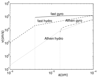
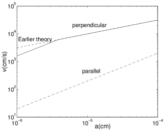
Figure 12: A new mechanism of grain acceleration is based on the direct interaction of charged grains with MHD turbulence. Gyroresonance of charged grains with fast modes dominates the acceleration of charged grains in Cold Neutral Medium (CNM). Within dark clouds the interaction of MHD turbulence and charged grains is important only for small grains. When grains decouple from magnetic field, Kolmogorov theory provides an OK estimate for grain velocities. From Yan & Lazarian YanL03 and Lazarian & Yan LazY02 .

9.4 Other examples: from HII regions to gamma ray busts

Lithwick & Goldreich LitG01 addressed the issue of the origin of density fluctuations within HII regions. There the gas pressure is larger than the magnetic pressure (the ‘high $\beta$’ regime) and they conjectured that fast waves, which are essentially sound waves, would be decoupled from the rest of the cascade. They found that density fluctuations are due to the slow mode and the entropy mode, which are passively mixed by shear Alfvén waves and follow a Kolmogorov spectrum. Our results in CL03 suggest that fast modes may be also an important source of density fluctuations. In addition, results on the new regime of turbulence (CLV02c, CL03) indicate that the new regime of turbulence can fluctuations on very small scales and this entails resumption of the turbulent cascade LazVC03 that was not considered in LitG01 .

The whole machinery of MHD turbulence scalings is required to deal with turbulence in gamma ray bursts (see LazPY03 ). There both fast and Alfven waves can transfer their energy to emitting electrons. However, the ways that they transfer their energy are different and this may result in important observational consequences.

Heating of ISM and of Diffuse Ionized Gas (DIG), in particular, is another issue where imbalanced MHD turbulence is important (see CLV02a). Compression of molecular clouds by MHD turbulence (see MyeL98 ), stochastic magnetic reconnection LazV99 ; LazVC03 are other examples when it is essential to know the fundamental properties of compressible MHD.

10 Summary

In the paper, we have studied generation of compressible MHD modes. We have presented the statistics of compressible MHD turbulence for high, intermediate, and low $\beta$ plasmas and for different sonic and Alfven Mach numbers. For subAlfvenic turbulence we provided the decomposition of turbulence into Alfven, slow and fast modes. We have found that the generation of compressible modes by Alfvenic modes is suppressed and, contrary to the common belief, the drain of energy from Alfven to compressible modes is marginal along the cascade. As the result the Alfvenic modes form a separate cascade with the properties similar to those of Goldreich-Sridhar cascade in incompressible media. As Alfven modes shear slow modes they impose their scaling on them. On the contrary, fast modes show isotropy for both magnetic- and gas-pressure dominated plasmas. The new insight into compressible MHD entails important astrophysical consequences that range from the dynamics of star formation to the dynamics of gamma ray busts.

Acknowledgments: We thank Ethan Vishniac, Peter Goldreich, Bill Matthaeus, Chris McKee, and Annick Pouquet for stimulating discussions. We acknowledge the support of NSF Grant AST-0125544. This work was partially supported by NCSA under AST010011N and utilized the NCSA Origin2000.

Appendix

Let us consider a small perturbation in the presence of a strong mean magnetic field. We write density, velocity, pressure, and magnetic field as the sum of constant and fluctuating parts: $\rho\rightarrow\rho_{0}+\rho$, ${\bf v}\rightarrow{\bf v}_{0}+{\bf v}$, $P\rightarrow P_{0}+p$, and ${\bf B}\rightarrow{\bf B}_{0}+{\bf b}$, respectively. We assume that ${\bf v}_{0}=0$ and that perturbation is small : $\rho<<\rho_{0}$, etc. Ignoring the second and higher order contributions, we can rewrite the MHD equations as follows:

$$\frac{\partial\rho}{\partial t}+\rho_{0}\nabla\cdot{\bf v}=0,$$ (47)

$$\rho_{0}\frac{\partial{\bf v}}{\partial t}+\nabla(a^{2}\rho)-\frac{1}{4\pi}(\nabla\times{\bf b})\times{\bf B}_{0}=0,$$ (48)

$$\frac{\partial{\bf b}}{\partial t}+\nabla\times\left[{\bf v}\times{\bf B}_{0}\right]=0,$$ (49)

where we assume a polytropic equation of state: $p=a^{2}\rho$ with $a^{2}=\gamma p_{0}/\rho_{0}$. We follow arguments in Thompson (1962) to derive magnetosonic waves. Let ${\bf\xi}({\bf r},t)$ be the displacement vector, so that $\partial{\bf\xi}/\partial t={\bf v}$. Assuming that the displacements vanish at $t=0$, we can integrate the equations as follows

$$\rho+\rho_{0}\nabla\cdot{\bf\xi}=0,$$ (50)

$$\ddot{\bf\xi}=a^{2}\nabla(\nabla\cdot{\bf\xi})+(\nabla\times{\bf b})\times{\bf B}_{0}/4\pi\rho_{0},$$ (51)

$${\bf b}=\nabla\times(\xi\times{\bf B}_{0}).$$ (52)

The momentum equation (eq. 51) becomes

$$\ddot{\bf\xi}=a^{2}\nabla(\nabla\cdot{\bf\xi})+\left[\nabla\times\left(\nabla\times(\xi\times{\bf B}_{0})\right)\right]\times{\bf B}_{0}/4\pi\rho_{0}$$ (53)

$$~{}~{}=a^{2}\nabla(\nabla\cdot{\bf\xi})+\nabla(B_{0}^{2}\nabla\cdot{\bf\xi}-{\bf B}_{0}\cdot\nabla{\bf B}_{0}\cdot{\bf\xi})/4\pi\rho_{0}$$ (54)

$$~{}~{}~{}-({\bf B}_{0}\cdot\nabla)^{2}{\bf\xi}/4\pi\rho_{0}+\left[{\bf B}_{0}({\bf B}_{0}\cdot\nabla)\nabla\cdot{\bf\xi}\right]/4\pi\rho_{0}$$ (55)

Using $\alpha=a^{2}/V_{A}^{2}=\beta(\gamma/2)$, $V_{A}=B_{0}/4\pi\rho_{0}$, we have

$$\ddot{\bf\xi}/V_{A}^{2}-\nabla[(\alpha+1)\nabla\cdot{\bf\xi}-(\hat{\bf B}_{0}\cdot\nabla)(\hat{\bf B}_{0}\cdot{\bf\xi})]\\ -(\hat{\bf B}_{0}\cdot\nabla)^{2}{\bf\xi}+(\hat{\bf B}_{0}\cdot\nabla)(\nabla\cdot{\bf\xi})\hat{\bf B}_{0}=0$$ (56)

In Fourier spacethe equation becomes

$$\ddot{\bf\xi}/V_{A}^{2}+k\hat{\bf k}[(\alpha+1)k\xi_{k}-k_{\|}\xi_{\|}]+k_{\|}^{2}{\bf\xi}-k_{\|}k\xi_{k}\hat{k}_{\|}=0,$$ (57)

where $\xi_{k}={\bf\xi}\cdot\hat{\bf k}$, $\xi_{\|}={\bf\xi}\cdot\hat{\bf k}_{\|}$, $\hat{\bf k}={\bf k}/k$, and $\hat{\bf k}_{\|}$ is unit vector parallel to ${\bf B}_{0}$ (i.e. $\hat{\bf k}_{\|}=\hat{\bf B}_{0}$). Assuming $\ddot{\bf\xi}=-\omega^{2}{\bf\xi}=-c^{2}k^{2}{\bf\xi}$, we can rewrite (57) as

$$(c^{2}/V_{A}^{2}-\cos^{2}\theta){\bf\xi}-[(\alpha+1)\xi_{k}-\cos\theta\xi_{\|}]\hat{\bf k}+\cos\theta\xi_{k}\hat{k}_{\|}=0,$$ (58)

where $\cos\theta=k_{\|}/k$ and $\theta$ is the angle between ${\bf k}$ and ${\bf B}_{0}$.

Using $\hat{\bf k}=\sin\theta\hat{\bf k}_{\perp}+\cos\theta\hat{\bf k}_{\|}$, we get

$$(c^{2}/V_{A}^{2}-\cos^{2}\theta){\bf\xi}-[(\alpha+1)\xi_{k}-\cos\theta\xi_{\|}]\sin\theta\hat{\bf k}_{\perp}$$ (59)

$$-\{[(\alpha+1)\xi_{k}-\cos\theta\xi_{\|}]\cos\theta-\cos\theta\xi_{k}\}\hat{\bf k}_{\|}=0.$$ (60)

Writing ${\bf\xi}=\xi_{\perp}\hat{\bf k}_{\perp}+\xi_{\|}\hat{\bf k}_{\|}+\xi_{\varphi}\hat{\bf\varphi}$, we get

$$(c^{2}/V_{A}^{2}-\cos^{2}\theta)\xi_{\perp}-[(\alpha+1)\xi_{k}-\cos\theta\xi_{\|}]\sin\theta=0,$$ (61)

$$(c^{2}/V_{A}^{2}-\cos^{2}\theta)\xi_{\|}-[\alpha\xi_{k}-\cos\theta\xi_{\|}]\cos\theta=0,$$ (62)

$$(c^{2}/V_{A}^{2}-\cos^{2}\theta)\xi_{\varphi}=0.$$ (63)

The non-trivial solution of equation (63) is the Alfven wave, whose dispersion relation is $\omega/k=V_{A}\cos\theta$. The direction of the displacement vector for Alfven wave is parallel to the azimuthal basis $\hat{\bf\varphi}$:

$$\hat{\bf\xi}_{A}=-\hat{\bf\varphi}=\hat{\bf k}_{\perp}\times\hat{\bf k}_{\|}.$$ (64)

Let us consider solutions of equations (61) and (62). Using $\xi_{k}=\xi_{\perp}\sin\theta+\xi_{\|}\cos\theta$, we get

$$(c^{2}/V_{A}^{2}-\cos^{2}\theta)\xi_{\perp}-(\alpha+1)\sin^{2}\theta\xi_{\perp}-\alpha\cos\theta\sin\theta\xi_{\|}=0,$$ (65)

$$(c^{2}/V_{A}^{2}-\cos^{2}\theta)\xi_{\|}-\alpha\sin\theta\cos\theta\xi_{\perp}-(\alpha-1)\cos^{2}\theta\xi_{\|}=0.$$ (66)

Rearranging these, we get

$$(c^{2}/V_{A}^{2}-\alpha\sin^{2}\theta-1)\xi_{\perp}-\alpha\cos\theta\sin\theta\xi_{\|}=0,$$ (67)

$$(c^{2}/V_{A}^{2}-\alpha\cos^{2}\theta)\xi_{\|}-\alpha\sin\theta\cos\theta\xi_{\perp}=0.$$ (68)

Combining these two, we get

$$(c^{2}/V_{A}^{2}-\alpha\sin^{2}\theta-1)(c^{2}/V_{A}^{2}-\alpha\cos^{2}\theta)$$ (69)

$$=\alpha^{2}\sin^{2}\theta\cos^{2}\theta.$$ (70)

Therefore, the dispersion relation is

$$c^{4}/V_{A}^{4}-(1+\alpha)c^{2}/V_{A}^{2}+\alpha\cos^{2}\theta=0.$$ (71)

The roots of the equation are

$$c_{f,s}^{2}=\frac{1}{2}V_{A}^{2}\left[(1+\alpha)\pm\sqrt{(1+\alpha)^{2}-4\alpha\cos^{2}\theta}\right],$$ (72)

where subscripts ‘f’ and ’s’ stand for ‘fast’ and ’slow’ waves, respectively.

We can write

$${\bf\xi}=\xi_{\|}\hat{\bf k}_{\|}+\xi_{\perp}\hat{\bf k}_{\perp}\propto\left[\frac{\xi_{\|}k_{\perp}}{\xi_{\perp}k_{\|}}\right]k_{\|}\hat{\bf k}_{\|}+k_{\perp}\hat{\bf k}_{\perp}.$$ (73)

Plugging eq. (72) into eq. (67) and (68), we get

$$\left[\frac{1+\alpha}{2}\pm\frac{\sqrt{D}}{2}-\alpha\sin^{2}\theta-1\right]\xi_{\perp}=\alpha\cos\theta\sin\theta\xi_{\|},$$ (74)

$$\left[\frac{1+\alpha}{2}\pm\frac{\sqrt{D}}{2}-\alpha\cos^{2}\theta\right]\xi_{\|}=\alpha\cos\theta\sin\theta\xi_{\perp},$$ (75)

where $D=(1+\alpha)^{2}-4{\alpha}\cos^{2}{\theta}$. Using $k_{\|}=k\cos\theta$ and $k_{\perp}=k\cos\theta$, we get

$$\left[\frac{-1+\alpha}{2}\pm\frac{\sqrt{D}}{2}\right]\xi_{\perp}k_{\|}-\alpha\sin^{2}\theta\xi_{\perp}k_{\|}=\alpha\cos^{2}\theta\xi_{\|}k_{\perp},$$ (76)

$$\left[\frac{1+\alpha}{2}\pm\frac{\sqrt{D}}{2}\right]\xi_{\|}k_{\perp}-\alpha\cos^{2}\theta\xi_{\|}k_{\perp}=\alpha\sin^{2}\theta\xi_{\perp}k_{\|}.$$ (77)

Arranging these, we get

$$\frac{\xi_{\|}k_{\perp}}{\xi_{\perp}k_{\|}}=\frac{-1+\alpha\pm\sqrt{D}}{1+\alpha\pm\sqrt{D}},$$ (78)

where the upper signs are for fast mode and the lower signs for slow mode. Therefore, we get

$$\hat{\bf\xi}_{s}\propto(-1+\alpha-\sqrt{D})k_{\|}\hat{\bf k}_{\|}+(1+\alpha-\sqrt{D})k_{\perp}\hat{\bf k}_{\perp},$$ (79)

$$\hat{\bf\xi}_{f}\propto(-1+\alpha+\sqrt{D})k_{\|}\hat{\bf k}_{\|}+(1+\alpha+\sqrt{D})k_{\perp}\hat{\bf k}_{\perp}.$$ (80)

The slow basis $\hat{\bf\xi}_{s}$ lies between $\hat{\bf k}_{\|}$ and $-\hat{\bf\theta}$. The slow basis $\hat{\bf\xi}_{f}$ lies between $\hat{\bf k}_{\perp}$ and $\hat{\bf k}$ (Fig. 3). Here overall sign of $\hat{\bf\xi}_{s}$ and $\hat{\bf\xi}_{f}$ is not important.

When $\alpha\rightarrow 0$, equations (80) and (79) becomes

$$\hat{\bf\xi}_{s}\approx\hat{\bf k}_{\|}-(\alpha\sin\theta\cos\theta)\hat{\bf k}_{\perp},$$ (81)

$$\hat{\bf\xi}_{f}\approx(\alpha\sin\theta\cos\theta)\hat{\bf k}_{\|}+\hat{\bf k}_{\perp}.$$ (82)

In this limit, $\hat{\bf\xi}_{s}$ is mostly proportional to $\hat{\bf k}_{\|}$ and $\hat{\bf\xi}_{f}$ to $\hat{\bf k}_{\perp}$. When $\alpha\rightarrow\infty$, equations (80) and (79) becomes

$$\hat{\bf\xi}_{s}\approx-\hat{\bf\theta}+(\sin\theta\cos\theta/\alpha)\hat{\bf k},$$ (83)

$$\hat{\bf\xi}_{f}\approx(\sin\theta\cos\theta/\alpha)\hat{\bf\theta}+\hat{\bf k}.$$ (84)

When $\alpha=\infty$, slow modes are called pseudo-Alfvenic modes.

We can obtain slow and fast velocity component by projecting Fourier velocity component ${\bf v}_{\bf k}$ onto $\hat{\bf\xi}_{s}$ and $\hat{\bf\xi}_{f}$, respectively.

To separate slow and fast magnetic modes, we assume the linearized continuity equation ($\omega\rho_{k}=\rho_{0}{\bf k}\cdot{\bf v}_{k}$) and the induction equation ($\omega{\bf b}_{k}={\bf k}\times({\bf B}_{0}\times{\bf v}_{k})$) are statistically true. From these, we get Fourier components of density and non-Alfvénic magnetic field:

$$\rho_{k} = (\rho_{0}\Delta v_{k,s}/c_{s})\hat{\bf k}\cdot\hat{\bf\xi}_{s}+(\rho_{0}\Delta v_{k,f}/c_{f})\hat{\bf k}\cdot\hat{\bf\xi}_{f}$$ (85)

$$\equiv \rho_{k,s}+\rho_{k,f},$$ (86)

$$b_{k} = (B_{0}\Delta v_{k,s}/c_{s})|\hat{\bf B}_{0}\times\hat{\bf\xi}_{s}|+(B_{0}\Delta v_{k,f}/c_{f})|\hat{\bf B}_{0}\times\hat{\bf\xi}_{f}|$$ (87)

$$\equiv b_{k,s}+b_{k,f},$$ (88)

$$= \rho_{k,s}(B_{0}/\rho_{0})(|\hat{\bf B}_{0}\times\hat{\bf\xi}_{s}|/\hat{\bf k}\cdot\hat{\bf\xi}_{s})$$ (89)

$$+ \rho_{k,f}(B_{0}/\rho_{0})(|\hat{\bf B}_{0}\times\hat{\bf\xi}_{f}|/\hat{\bf k}\cdot\hat{\bf\xi}_{f}),$$ (90)

where $\Delta v_{k}\propto v_{k}^{+}-v_{k}^{-}$ (superscripts ‘+’ and ‘-’ represent opposite directions of wave propagation) and subscripts ‘s’ and ‘f’ stand for ‘slow’ and ‘fast’ modes, respectively. From equations (86), (88), and (90), we can obtain $\rho_{k,s}$, $\rho_{k,f}$, $b_{k,s}$, and $b_{k,f}$ in Fourier space.

References

- (1) J. W. Armstrong, B. J. Rickett, S. R. Spangler: Astrophys. J. 443, 209 (1995)
- (2) C. Baccigalupi, C. Burigana, F. Perrotta, G. De Zotti, L. La Porta, D. Maino, M. Maris, R. Paladini: Astron. Astrophys. 372, 8 (2001)
- (3) F. Bataille, Y. Zhou: Phys. Rev. E 59(5), 5417 (1999)
- (4) J.-P. Bertoglio, F. Bataille, J.-D. Marion: Phys. Fluids 13, 290 (2001)
- (5) B. Chandran: Phys. Rev. Lett. 85(22), 4656 (2001)
- (6) J. Cho, A. Lazarian: Phy. Rev. Lett. 88, 245001 (2002a) (CL02)
- (7) J. Cho, A. Lazarian: Astrophys. J. 575, L63 (2002)
- (8) J. Cho, A. Lazarian: submitted to Monthly Not. Roy. Astron. Soc. (2003) (http://xxx.lanl.gov/abs/astro-ph/0301062) (CL03)
- (9) J. Cho, A. Lazarian, E. Vishniac: in Simulations of magnetohydrodynamic turbulence in astrophysics, eds. T. Passot & E. Falgarone (Springer LNP) (2002a) (astro-ph/0205286) (CLV02a)
- (10) J. Cho, A. Lazarian, E. Vishniac: Astrophys. J. 564, 291 (2002b) (CLV02b)
- (11) J. Cho, A. Lazarian, E. Vishniac: Astrophys. J. 566, L49 (2002c) (CLV02c)
- (12) J. Cho, E. Vishniac: Astrophys. J. 538, 217 (2000a)
- (13) J. Cho, E. Vishniac: Astrophys. J. 539, 273 (2000b)
- (14) L. Del Zanna, M. Velli, P. Londrillo: Astron. Astrophys. 367, 705 (2001)
- (15) A. A. Deshpande: Monthly Not. Roy. Astron. Soc. 317, 199 (2000)
- (16) A. A. Deshpande, K. S. Dwarakanath, W. M. Goss: Astrophys. J. 543, 227 (2000)
- (17) R. L. Dickman: in Protostars and Planets II, ed. by D. C. Black, M. S. Mathews (Tucson: Univ. Arizona Press, 1985) p.150
- (18) B. Draine, A. Lazarian: Astrophys. J. 508, 157 (1998)
- (19) W. J. Feiereisen, E. Shirani, J. H. Ferziger, W. C. Reynolds: in Turbulent Shear Flows 3, (Springer), p. 309 (1982)
- (20) P. Fosalba, A. Lazarian, S. Prunet, J. A. Tauber: Astron. J. 564, 762 (2002)
- (21) G. Giardino, A.J. Banday, P. Fosalba, K.M. Górski, J.L. Jonas, W. O’Mullane, J. Tauber: Astron. Astrophys. 371 708 (2001)
- (22) G. Giardino, A.J. Banday, K.M. Górski, K. Bennett, J.L. Jonas, J. Tauber: Astron. Astrophys. (astro-ph/0202520) (2002)
- (23) P. Goldreich, P. Kumar: Astrophys. J. 363, 694 (1990)
- (24) P. Goldreich, S. Sridhar: Astrophys. J. 438, 763 (1995)
- (25) P. Goldreich, S. Sridhar: Astrophys. J. 485, 680 (1997)
- (26) M. L. Goldstein, D. A. Roberts: Annu. Rev. Astron. Astrophys. 33, 283, (1995)
- (27) J. Goodman, R. Narayan: Monthly Not. Roy. Astron. Soc. 214, 519 (1985)
- (28) D. A. Green: Monthly Not. Roy. Astron. Soc. 262, 328 (1993)
- (29) J. C. Higdon: Astrophys. J. 285, 109 (1984)
- (30) S. von Horner: Zs.F. Ap. 30, 17 (1951)
- (31) T. S. Horbury, A. Balogh: Nonlin. Proc. Geophys. 4, 185 (1997)
- (32) T. S. Horbury: in Plasma Turbulence and Energetic particles, ed. by M. Ostrowski, R. Schlickeiser (Cracow, Poland, 1999) p.28
- (33) G. Jiang, C. Wu: J. Comp. Phys. 150, 561 (1999)
- (34) B. B. Kadomtsev, V. I. Petviashvili: Sov. Phys. Dokl. 18, 115 (1973)
- (35) J. Kampé de Fériet: in: Gas Dynamics of Cosmic Clouds (Amsterdam: North-Holland, 1955) p.134
- (36) S. A. Kaplan, S. B. Pickelner: The Interstellar Medium (Harvard Univ. Press, 1970)
- (37) S. Kida, S. A. Orszag: J. Sci. Comput. 5(1), 1 (1990a)
- (38) S. Kida, S. A. Orszag: J. Sci. Comput. bf 5(2), 85 (1990b)
- (39) L. Klein, R. Bruno, B. Bavassano, H. Rosenbauer: J. Geophys. Res. 98, 17461 (1993)
- (40) A. Kolmogorov: Dokl. Akad. Nauk SSSR 31, 538 (1941)
- (41) R. B. Larson: Monthly Not. Roy. Astron. Soc. 194, 809 (1981)
- (42) A. Lazarian: Astron. Astrophys. 293, 507 (1995)
- (43) A. Lazarian: in Interstellar Turbulence, ed. by J. Franco, A. Carraminana (Cambridge Univ. Press, 1999a) p.95 (astro-ph/9804024)
- (44) A. Lazarian: in Plasma Turbulence and Energetic Particles, ed. by M. Ostrowski, R. Schlickeiser (Cracow, 1999b) p.28, (astro-ph/0001001)
- (45) A. Lazarian: in Cosmic Evolution and Galaxy Formation, ASP v.215, ed. by J. Franco, E. Terlevich, O. Lopez-Cruz, I. Aretxaga (Astron. Soc. Pacific, 2000) p.69 (astro-ph/0003414)
- (46) A. Lazarian, J. Cho, H. Yan: preprint (astro-ph/0211031) (2003)
- (47) A. Lazarian, A. Goodman, P. Myers: Astrophys. J. 490, 273 (1997)
- (48) A. Lazarian, V. Petrosian, H. Yan, J. Cho: preprint (astro-ph/0301181) (2003)
- (49) A. Lazarian, D. Pogosyan: Astrophys. J. 537, 720L (2000)
- (50) A. Lazarian, D. Pogosyan: (2003), in preparation
- (51) A. Lazarian, D. Pogosyan, A. Esquivel: in Seeing Through the Dust, ed. by R. Taylor, T. Landecker, A. Willis (ASP Conf. Series, 2002), in press (astro-ph/0112368) (LPE02)
- (52) A. Lazarian, D. Pogosyan, E. Vazquez-Semadeni, B. Pichardo: Astrophys. J. 555, 130 (2001)
- (53) A. Lazarian, V. R. Shutenkov: Sov. Astron. Lett. 16(4), 297 (1990)
- (54) A. Lazarian, E. Vishniac: Astrophys. J. 517, 700 (1999)
- (55) A. Lazarian, E. Vishniac, J. Cho: Astrophys. J., submitted
- (56) A. Lazarian, H. Yan: Astrophys. J. 566, 105 (2002)
- (57) R. J. Leamon, C. W. Smith, N. F. Ness, W. H. Matthaeus, H. Wong: J. Geophys Res. 103, 4775 (1998)
- (58) J. Lee: Astrophys. J. 404, 372 (1993)
- (59) M. Lee, S. K. Lele, P. Moin: Phys. Fluids A 3, 657 (1991)
- (60) M. J. Lighthill: Proc. Roy. Soc. London A 211, 564 (1952)
- (61) Y. Lithwick, P. Goldreich: Astrophys. J. 562, 279 (2001)
- (62) X. Liu, S. Osher: J. Comp. Phys. 141, 1 (1998)
- (63) V. S. L’vov, Y. V. L’vov, A. Pomyalov: Phys. Rev. E 61, 2586 (2000)
- (64) M.-M. Mac Low, R. Klessen: preprint (astro-ph/0301093) (2003)
- (65) M.-M. Mac Low, R. Klessen, A. Burkert, M. Smith: Phy. Rev. Lett. 80, 2754 (1998)
- (66) C. F. McKee: in The Origin of Stars and Planetary Systems, ed. by J. L. Charles, D. K. Nikolaos (Dordrecht: Kluwer, 1999) p.29
- (67) J. Maron, P. Goldreich: Astrophys. J. 554, 1175 (2001)
- (68) W. H. Matthaeus, M. R. Brown: Phys. Fluids 31(12), 3634 (1988)
- (69) W. M. Matthaeus, S. Ghosh, S. Oughton, D. A. Roberts: J. Geophys. Res. 101, 7619 (1996)
- (70) W. H. Matthaeus, M. L. Goldstein, D. C. Montgomery: Phys. Rev. Lett. 51, 1484 (1983)
- (71) W. M. Matthaeus, S. Oughton, S. Ghosh, M. Hossain: Phy. Rev. Lett. 81, 2056 (1998)
- (72) C. F. McKee: in The Origin of Stars and Planetary Systems, ed. by J. L. Charles, D. K. Nikolaos (Dordrecht: Kluwer, 1999) p.29
- (73) A. Minter, S. Spangler: Astrophys. J. 485, 182 (1997)
- (74) S. S. Moiseev, V. I. Petviashvili, A. V. Toor, V. V. Yanovsky: Physica 2D, 218 (1981)
- (75) A. S. Monin, A. A. Yaglom: Statistical Fluid Mechanics: Mechanics of Turbulence, Vol. 2 (Cambridge: MIT Press, 1975)
- (76) J. E. Moyal: Proc. Camb. Phil. Soc. 48, 329 (1951)
- (77) W. Müller, D. Biskamp: Phys. Rev. Lett. bf 84, 475 (2000)
- (78) G. Munch: Rev. Mod. Phys. 30, 1035 (1958)
- (79) Z. E. Musielak, R. Rosner: Astrophys. J. 329, 376 (1988)
- (80) Z. E. Musielak, R. Rosner, & P. Ulmschneider: Astrophys. J., 337, 470 (1989)
- (81) P. Myers, A. Lazarian: Astrophys. J. 507, L157 (1998)
- (82) R. Narayan, J. Goodman: Monthly Not. Roy. Astron. Soc. 238, 963 (1989)
- (83) T. Passot, A. Pouquet: J. Fluid Mech. 181, 441 (1987)
- (84) T. Passot, A. Pouquet, P. Woodward: Astron. Astrophys. 197, 228 (1988)
- (85) T. Passot, E. Vazquez-Semadeni: preprint (astro-ph/0208173) (2002)
- (86) D. Porter, A. Pouquet, P. Woodward: Phys. Rev. Lett. 68, 3156 (1992)
- (87) D. Porter, A. Pouquet, P. Woodward: Phys. Rev. E 66, 026301 (2002)
- (88) D. Porter, P. Woodward, A. Pouquet: Phys. Fluids 10, 237 (1998)
- (89) S. Sarkar, G. Erlebacher, M. Y. Hussaini, H. O. Kreiss: J. Fluid Mech. 227, 473 (1991)
- (90) A. Schekochihin, J. Maron, S. Cowley, J. McWilliams: Astrophys. J. 576, 806 (2002)
- (91) A. Schlickeiser, J. A. Miller: Astrophys. J. 492, 352 (1998)
- (92) J. V. Shebalin, W. H. Matthaeus, D. C. Montgomery: J. Plasma Phys. 29, 525 (1983)
- (93) S. R. Spangler, C. R. Gwinn: Astrophys. J. 353, L29 (1990)
- (94) S. Stanimirovic, A. Lazarian: Astrophys. J. 551, L53 (2001)
- (95) I. Staroselsky, V. Yakhot, S. Kida, S. A. Orszag: Phy. Rev. Lett. 65, 171 (1990)
- (96) R. F. Stein: Sol. Phys. 2, 385 (1967)
- (97) J. Stone, E. Ostriker, C. Gammie: Astrophys. J. 508, L99 (1998)
- (98) W, B. Thompson: An Introduction to Plasma Physics, (Pergamon Press) (1962)
- (99) E. Vazquez-Semadeni, E. C. Ostriker, T. Passot, C. F. Gammie, J. M. Stone: in Protostars and Planets IV, eds. V. Mannings et al. (Tucson: University of Arisona Press), p.3 (2000)
- (100) O. C. Wilson, G. Munch, E. M. Flather, M. F. Coffeen: Astrophys. J. Supp. 4, 199 (1959)
- (101) H. Yan, A. Lazarian: Phys. Rev. Lett.89, 281102 (2002)
- (102) H. Yan, A. Lazarian: preprint (astro-ph/0301007) (2003)
- (103) V. E. Zakharov: Sov. Phys. JETP 24, 455 (1967)
- (104) V. E. Zakharov, A. Sagdeev: Sov. Phys. Dokl. 15, 439 (1970)
- (105) G. P. Zank, W. H. Matthaeus: Phys. Fluids A 5(1), 257 (1993)
- (106) E. Zweibel, F. Heitsch, Y. Fan: preprint (astro-ph/0202525) (2002)