Image Simulation with Shapelets

Abstract

We present a method to simulate deep sky images, including realistic galaxy morphologies and telescope characteristics. To achieve a wide diversity of simulated galaxy morphologies, we first use the shapelets formalism to parametrize the shapes of all objects in the Hubble Deep Fields. We measure this distribution of real galaxy morphologies in shapelet parameter space, then resample it to generate a new population of objects. These simulated galaxies can contain spiral arms, bars, discs, arbitrary radial profiles and even dust lanes or knots. To create a final image, we also model observational effects, including noise, pixellisation, astrometric distortions and a Point-Spread Function. We demonstrate that they are realistic by showing that simulated and real data have consistent distributions of morphology diagnostics: including galaxy size, ellipticity, concentration and asymmetry statistics. Sample images are made available on the world wide web. These simulations are useful to develop and calibrate precision image analysis techniques for photometry, astrometry, and shape measurement. They can also be used to assess the sensitivity of future telescopes and surveys for applications such as supernova searches, microlensing, proper motions, and weak gravitational lensing.

1 Introduction

As astronomical surveys are growing in size and scope, so image analysis methods are increasing in complexity and accuracy. In order to calibrate these new methods, it is essential to have a large sample of images containing objects whose properties are already known. Since real data is subject to the uncertainties of observational noise, telescope aberration and seeing, several packages have been developed to manufacture artificial images (e.g. Skymaker (see Erben et al. 2001) or artdata in IRAF (Tody 1993)). The accuracy of image analysis methods can then be assessed by comparing their output to the known input image properties that were specified before the addition of such observational effects.

The image simulation packages currently available are particularly valuable for imitating deep ground-based data. However, they limit themselves to a representation of galaxies as parametric forms such as symmetric de Vaucouleurs or exponential profiles. Deep space-based images, on the other hand, contain many irregular or asymmetrical galaxies with complex resolved features such as spiral arms, mergers and dust lanes. One possibility for simulating space images, utilised by Bouwens, Broadhurst & Silk (1998), is to repeatedly reuse well-resolved galaxies from the Hubble Deep Fields (HDFs; Williams et al. 1996, 1998). However, this restricts us to morphology templates from a relatively bright and nearby sample. Fainter galaxies cannot be used because they have been significantly contaminated with background noise. Consequently, the morphological properties of the faint galaxy population are not fairly represented. This method also faces the difficulty that the same real galaxies must be reused many times within one simulation. Although the HDFs are indeed very deep ($I_{F814W}$=27.60 at 10$\sigma$, Williams et al. 1996), they only cover a small area ($\sim$6 square arcminutes each) and contain a finite number of galaxies. Even if we were to source our real galaxies from larger surveys such as the Groth strip (Groth et al. 1994) or the Medium Deep Survey (Ratnatunga, Griffiths & Ostrander 1999), we would still face the difficulty of using particular real galaxies many times in a large simulation.

In this paper, we present a method for simulating deep images that contain genuinely unique objects, yet replicate the morphological distribution of galaxies in the HDF at all depths. This method has the advantage of allowing us to simulate arbitrarily large, deep surveys with no repetition of galaxy shapes. It also allows us to know accurately the intrinsic properties of each galaxy, before adding telescope-specific noise properties, systematic effects and convolution with a Point-Spread Function (PSF).

Our method is to decompose all objects in the HDFs into shapelet parametrizations, following the formalism introduced by Refregier (2003, hereafter Shapelets I) and Refregier & Bacon (2003; hereafter Shapelets II). Using just a few coefficients, these can completely quantify the shape properties of all galaxies, including spiral arms, bars and arbitrary radial profiles. We then model their distribution of shapelet coefficients, and draw from this probability distribution new sets of shapelet coefficients, representing new galaxies. In particular, we take into account the covariance between shapelet coefficients so that, for example, shapes depend upon magnitude and size (e.g. faint galaxies appear more irregular than bright ones). In this method, we therefore do not input any model of physical morphology or evolution. Rather, we exclusively use the measured statistics of the shapelet coefficient distributions from a real galaxy sample, as a function of magnitude and size. The new galaxy images can then be analytically convolved with any PSF, pixellated, and given an appropriate amount of noise for any exposure time down to the depth of the HDF.

These simulations have several significant applications. We can use them to calibrate the effectiveness of image analysis and detection methods such as SExtractor (Bertin & Arnouts 1996), imcat (Kaiser, Squire & Broadhurst 1995), GIM2D (Simard 1998), GALFIT (Peng et al. 2002) and wavelet routines (e.g. Meyer 1993). By examining the errors on shape measurement at various signal-to-noise levels of galaxy detection, we can also predict the accuracy of future experiments requiring accurate shape measurement. An example of this for space-based cosmic shear surveys is presented in Massey et al. (2003).

This paper is organized as follows. In §2 we give a brief overview of the shapelet formalism and describe how the HDF galaxies are modelled using shapelet coefficients. In §3, we show how the properties of the shapelet basis functions make them eminently suitable for this method. In §4 we discuss the means by which we recover a smooth probability distribution of galaxy morphologies in shapelet parameter space. In §5 we generate new galaxies by resampling the distribution. We then add observational noise and show an example of the final simulated images.

We then demonstrate that the simulations do indeed have similar properties to the HDFs. For this purpose, we consider in §6 commonly used quantifiers for galaxy morphology. We find good agreement between simulations and the real HDF galaxies for measures such as the size-magnitude distribution, ellipticity, concentration, asymmetry and clumpiness indices (e.g. Bershady et al. 2000, Conselice et al. 2000a). It is this agreement which is the final justification of our shapelet-based simulation method. We compare our method to others in §7 and summarise our findings in §8. Sample images may be downloaded from http://www.ast.cam.ac.uk/$\sim$rjm/shapelets.

2 Shapelet source catalogue

In this section, we describe the detection of HDF galaxies and their modelling as shapelets. This procedure creates a parametrized catalogue of real galaxy morphologies, which we will require later.

2.1 Source detection

Objects are initially detected using SExtractor (Bertin & Arnouts 1996) upon the HDF $I$-band (F814W) images, together with the pixel weight maps outputted by DRIZZLE (Fruchter & Hook 2002). The convolution mask and detection parameters were adapted from those used by Williams et al. (1996). In particular, we use a comparatively low S/N detection threshold, ${\mathrm{D}ETECT\_THRESH}$, of 1.3. This affords recovery of faint galaxies and minimizes incompleteness, at the expense of many false-positive ‘detections’ of noise, which need to be flagged and filtered out later (see §2.2). Stars with ${\mathrm{C}LASS\_STAR}>97$% are immediately discarded, as we wish to model only galaxies. The image is then segmented into small square ‘postage stamp’ regions around the remaining galaxies. The sizes of these regions are set to $(3\times{\mathrm{A}\_IMAGE}+5)$ pixels square, where ${\mathrm{A}\_IMAGE}$ is a measure of the galaxy’s major axis provided by SExtractor. This area is slightly smaller than those illustrated in figure 1; it is compact enough to be computationally efficient, but large enough to ensure that the shapelet basis functions are close to zero at the boundaries of the image.

This prescription conveniently leaves a border of sky background and noise around the edge of each image. We use all of the border pixels that do not belong to any other object in the SExtractor catalogue to locally renormalise the pixel weight map. As noticed by Williams et al. (1996), the inverse variance map outputted during the data reduction of the HDF systematically overestimates the noise by a factor of a few. This bias also varies as a function of position around the image. While SExtractor requires only relative weights between pixels, and is thus unaffected by this bias, we need to calibrate the absolute value of noise for the shapelet decomposition.

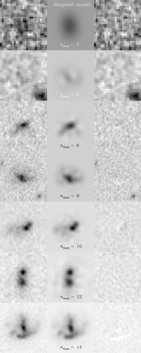
Figure 1: Shapelet modelling of a selection of HDF $I$-band galaxies. Higher S/N galaxies typically require more shapelet coefficients so we display a variety of source galaxies, noting the shapelet $n_{\rm max}$ required to reach a reconstruction with $\chi^{2}_{r}=1$. In all cases, the first column shows the original HDF image; the middle column shows the shapelet model; the right column shows the residual. The image size and colour scale is different for each row.

2.2 Shapelet modelling

Shapelets are a complete, orthonormal set of 2D basis functions. A linear combination of these functions can be used to model any image, in a similar way to Fourier or wavelet synthesis. The shapelet decomposition is particularly efficient for images localised in space, such as those of individual galaxies. The formalism was first introduced in Shapelets I, and a related method has also been independently suggested by Bernstein & Jarvis (2002).

For the polar shapelet analysis, the surface brightness $f({\mathbf{x}})$ of an object can be written as

$$f({\mathbf{x}})=\sum_{n=0}^{\infty}\sum_{m=-n}^{n}a_{nm}\chi_{nm}({\mathbf{x}}-{\mathbf{x}}_{c};\beta)~{},$$ (1)

where $\beta$ is a scale parameter, and ${\mathbf{x}}_{c}$ is the position of the centre of the basis functions. Only combinations of $n$ and $m$ where both are even or both are odd should be included in this summation. The basis functions $\chi_{nm}$, expressed in their polar separable form, are given by

$$\chi_{n,m}(r,\theta;\beta)=~{}~{}~{}~{}~{}~{}~{}~{}~{}~{}~{}~{}~{}~{}~{}~{}~{}~{}~{}~{}~{}~{}~{}~{}~{}~{}~{}~{}~{}~{}~{}~{}~{}~{}~{}~{}~{}~{}~{}~{}~{}~{}~{}~{}~{}~{}~{}~{}~{}~{}~{}$$

$$\frac{(-1)^{\frac{n-|m|}{2}}}{\beta^{|m|+1}\sqrt{\pi}}\left[\frac{\left(\frac{n-|m|}{2}\right)!}{\left(\frac{n+|m|}{2}\right)!}\right]^{\frac{1}{2}}r^{|m|}L_{\frac{n-|m|}{2}}^{|m|}\left(\frac{r^{2}}{\beta^{2}}\right)e^{\frac{-r^{2}}{2\beta^{2}}}e^{im\theta},$$ (2)

where $L(x)$ are the Laguerre polynomials (see e.g. Boas 1983). The index $n$ describes the radial oscillations and the index $m$ describes the order of rotational symmetry. Orthonormality ensures that the shapelet coefficients $a_{nm}$ are given by

$$a_{n,m}=\int_{0}^{2\pi}d\theta\int_{0}^{\infty}r~{}dr~{}f(r,\theta)~{}\chi_{n,m}(r,\theta;\beta)~{}.$$ (3)

These are Gaussian-weighted multipole moments of the surface brightness, familiar in several branches of astronomy.

For reasonable choices of the centroid ${\mathbf{x}}_{c}$ and scale size $\beta$, the galaxy shape information is contained within only the first few shapelet coefficients. The series in equation (1) can then be truncated at some finite order $n_{\rm max}$. In order to make good choices for ${\mathbf{x}}_{c}$, $\beta$ and $n_{\rm max}$, we first define $\chi^{2}_{r}$ as the difference between the original and reconstructed image, renormalised with respect to the local noise level. We then attempt to find the values of ${\mathbf{x}}_{c}$ and $\beta$ which achieve $\chi^{2}_{r}=1$ with the fewest possible shapelet coefficients, or minimum $n_{\rm max}$. Shapelet coefficients with higher $n$ can be discarded and the shapelet model will still be consistent with the data.

A practical algorithm to perform this optimisation by iteratively exploring $\{{\mathbf{x}}_{c}$, $\beta$, $n_{\rm max}\}$ space is described in Massey & Refregier (2003). The algorithm creates a catalogue of optimised shapelet decompositions for $\sim 500$ objects per square arcminute in the HDFs. However, this represents only 81% of the ‘objects’ detected by SExtractor. Approximately two dozen of the brightest of these galaxies require a decomposition with $n_{\rm max}>15$ to achieve $\chi^{2}_{r}\leq 1$. To reduce the dimensionality in later analysis, these parametrizations are truncated at this point regardless, with ${\mathbf{x}}_{c}$ and $\beta$ chosen to give the best possible, if slightly imperfect, shapelet fit. The algorithm also fails to converge to fits with $\chi^{2}_{r}\leq 1$ for a further 42 galaxies in close pairs, as identified by the SExtractor segmentation map; 36 galaxies because of their proximity to bright stars or the edge of the image; and 60 more objects across the HDFs (about 10% of all SExtractor detections), which are mainly false detections of noise due to the low S/N detection threshold set in section §2.1. Note that the number of decompositions which fail due to contamination from a near neighbour is roughly independent of magnitude. Indeed, the slope of the number counts for galaxy pair members is within $1\sigma$ of that for all the galaxies in the HDF: therefore this particular effect should not introduce any bias.

Figure 1 displays a selection of HDF galaxies at various S/N levels, and their shapelet reconstructions (see also Shapelets I, figures 3 and 4). Faint galaxies typically require an $n_{\rm max}$ of only 2, 3 or 4, while brighter, larger objects require an increasing number of shapelet coefficients to model their greater degree of detail. The right-hand column of figure 1 shows the reconstruction residuals, which are consistent with noise even for irregular galaxy morphologies.

2.3 Treatment of the PSF

During the modelling of galaxy shapes, we must in general account for the PSF of the WFPC2 camera that has smeared the HDF images. Since our objective here is to simulate only HST images, we do not apply any correction. The PSF will be naturally contained within the shapelet parametrization of the galaxy images and these are intentionally left unaltered. When we create simulated images, they will automatically have been smeared by the WFPC2 PSF: effectively circularised on average, because of the random reorientation of the new galaxies.

However, for other applications it may be desir able to simulate observations from other telescopes such as the JWST (http://www.stsci.edu/ngst/), SNAP (http://snap.lbl.gov/) or GAIA (http://astro. esa.int/gaia/). It would then be necessary to take account of their different instrumental properties. The ideal way to do this would be to deconvolve HDF galaxies from the WFPC2 PSF analytically in shapelet space (see Shapelets II §3), and then to reconvolve simulated galaxies with a new PSF at the end. Unfortunately, we have found this method difficult to implement in practice. The process of deconvolution naturally pushes information into high-$n$ and $m$ shapelet coefficients, as shown in Shapelets I figure 8. Although the ensuing galaxy reconstructions are still realistic, information about the overall galaxy morphology distribution is spread thinly over an increased number of coefficients. This distribution is no longer sufficiently well sampled by galaxies in the HDFs for the smoothing-and-resampling method presented in §4 to be effective.

An alternative solution exists to simulate images with a PSF of the same size or larger than that of HST. The WFPC2 PSF can be conveniently maintained throughout the simulations, and the images convolved again at the end with a second, ‘difference’ kernel. This kernel is intended to make up the difference between the original PSF of WFPC2 and that of the new instrument. It can be obtained by deconvolving the WFPC2 PSF from the new PSF, an operation performed easily in shapelet space (see Shapelets II §3). An example of this method can be seen in Massey et al. 2003.

3 Advantages and disadvantages of using shapelets

3.1 Advantages of shapelets

Figure 1 demonstrates the superb quality of shapelet-based image reconstruction possible for all galaxy morphologies. Particularly for spiral or irregular galaxies, we find the shapelet models superior to those using traditional radial profiles alone e.g. GALFIT (Peng et al. 2002). That paper contains plots similar to figure 1; but with much worse residuals.

There are also many more advantages to using the shapelet parametrization for image simulations. For example, the truncation in $n_{\rm max}$ produces data compression by setting a minimum and maximum physical scale of interest (see discussion in Shapelets I). The discarded high-$n$ order coefficients contain a small amount of high spatial frequency information. But because we have ensured that the reconstruction has been pursued up to an order $n_{\rm max}$ such that $\chi^{2}_{r}\leq 1$, we know that the high-frequency remainder is consistent with noise. Usefully for astronomy, the resolution of a shapelet model is also greatest near its centre. The compression factor for typical galaxy morphologies can be as high as $50$ (Shapelets I). Furthermore, this compression is achieved through a parameter-independent truncation of a series. With its complete basis set, shapelets avoid the requirement in GALFIT or GIM2D (Simard 1998) to specify in advance the number and type of profiles for each model. A Karhunen-Loéve decomposition would also require models to be specified in advance for both the image and the noise. Furthermore, the orthonormality of the shapelet basis set guarantees a unique and linear one-to-one mapping from the image plane to the coefficients. This advantage, and many of shapelets’ convenient mathematical properties are lost to methods using an over-complete basis set such as Pixon (Piña & Puetter 1993).

It is mainly for these convenient mathematical properties that we choose to model galaxies using shapelets. For example, an object’s orientation is controlled to first order by the phase of the $a_{22}$ coefficient (corresponding to the position angle of the object’s ellipticity); and its chirality (handedness) by the relative phase of the $a_{42}$ coefficient. The first can easily be factored out of the parametrization, so that the ellipticity of all objects becomes aligned to the horizontal axis. The image can then be flipped, if necessary, so that the sign of the $a_{42}$ phase is positive and the outer isophotes of all objects twist in the same anti-clockwise sense. Correlations between remaining shapelet coefficients $a_{nm}$ are of course maintained in order to preserve the morphology of the galaxy. Any two well-sampled objects which are identical apart from their orientation will then decompose into identical shapelet coefficients. This greatly increases the sampling density of the galaxy morphology distribution. Simulated galaxies will later be randomly rerotated and flipped as they are created.

Shapelets are also designed to be convenient for many aspects of image manipulation and post-processing. Since the shapelet basis functions $\chi_{nm}$ are the eigenfunctions of the 2D Quantum Harmonic Oscillator, they are invariant under Fourier transform up to a phase factor. This renders convolutions (e.g. with a PSF) easy and quick to perform. It also suggests a well-developed mathematical notation from quantum mechanics. Convolutions become a bra-ket matrix multiplication (see Shapelets II). Translations and rotations, useful for simulating dithered images, are described to first order by a few applications of $\hat{a}$ and $\hat{a}^{\dagger}$ ladder operators. So too are the distorting shears produced by both optical aberrations within a telescope and weak gravitational lensing within galaxy clusters (see Shapelets I).

3.2 Disadvantages of shapelets

There are two main criticisms often levelled at shapelets. The first is that a Gaussian-Laguerre expansion may not easily capture the extended wings of many galaxies. After truncation in $n_{\rm max}$, the shapelet basis set is left incomplete and not ideally matched to typical exponential or de Vaucouleurs profiles. A demonstration that our algorithm does select sufficiently high $n_{\rm max}$ is the remarkable match in the concentration index between shapelet models and real galaxies shown in §6. In fact, the ability of a shapelet decomposition to recognise correlations between adjacent pixels may even enable it to extend further than SExtractor into the wings of a faint object at the threshold of detection, where flux in individual pixels is lost beneath the noise.

A potentially greater problem for our simulations is the second criticism that a shapelet decomposition can produce artefacts when it is truncated. Indeed, any truncated basis set that is complete rather than over-complete will be subject to spurious residuals that resemble one basis state, due to the near-cancelling of large positive and negative coefficients in others. For shapelets, this emerges as ringing, and is particularly apparent after PSF deconvolution or around long and thin galaxies, which are less well-matched to the circular basis functions. Furthermore, a desire to keep the shapelet decomposition method linear prevents the imposition of a positive-definite constraint. The spurious residuals can therefore appear as either extra positive flux or negative holes. However, we note that this occurs widely in other methods, including wavelets, where it is only removed by a (non-linear) projection in wavelet space onto the sub-space of positive solutions. While most low-level residuals will be lost in the final simulated images beneath even modest background noise, we turn around this disadvantage in §5.1. There we use the absence of any negative holes in a noise-free image as a first-order diagnostic that the morphed shapes of simulated galaxies are realistic.

4 Shapelet parameter space

4.1 The multi-dimensional Hubble Tuning Fork

A sample of galaxy morphologies can be thought of as a distribution of points in a multi-dimensional shape parameter space. The axes in this space might represent size, magnitude, position angle (P.A.) and so on. Each point corresponds to a particular galaxy with a specific morphology, and various correlations may emerge between variables. For example, the classic Hubble tuning-fork diagram (Hubble 1926, Sandage 1961, de Vaucouleurs 1959) relates the object ellipticity, the bulge/disc ratio, and the extent to which the spiral arms are unwound. GIM2D (Simard 1998) and GALFIT (Peng 2002) software use axes parametrized by the relative amounts of exponential or de Vaucouleurs/Sérsic functions (de Vaucouleurs 1959, Sérsic 1968) required to fit the galaxy’s radial profile.

4.2 The multi-dimensional Shapelet Tuning Fork

In this work, we instead choose the axes of our galaxy morphology distribution to be the magnitudes and complex phases of the polar shapelet coefficients. First, we describe the properties of this ‘shapelet parameter space’. In the following section, we will then argue that the underlying Probability Density Function (PDF) of galaxy morphology is relatively simple in this parameter space and may be recovered from a finite sample like the HDFs.

Projections of shapelet parameter space are shown in figure 2. Each point in the top-left panel represents a data vector encoding the shape information about one HDF galaxy. Collectively, they describe the overall morphology distribution of distant galaxies. The rotations and reflections used to pre-align galaxies have considerably compressed this space (without loss of information) and allowed it to be more densely sampled by only a finite number of galaxies. Notice that there are correlations evident in the parameters, which correspond to the construction of the familiar shapes of galaxies. In the middle-left plot, for example, the scatter of ellipticity values widens for faint galaxies which are known to be more irregular. In the bottom-right plot, deviations from the diagonal show twisting isophotes that can grow, with higher order basis functions, into spiral arms. It is also important to notice that some regions of parameter space are empty. A random set of shapelet coefficients will not produce a realistic galaxy shape: there is not even a positive definite constraint imposed upon an image in the shapelet formalism.

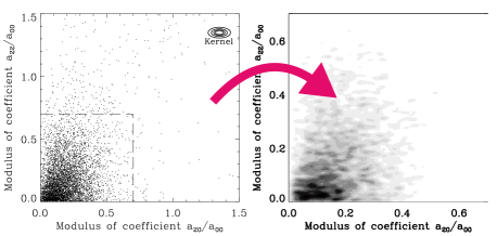
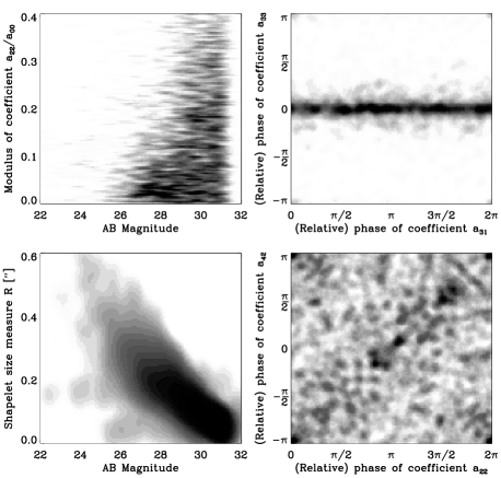
Figure 2: Phase space correlations and smoothing in the shapelet parameter space. The top left panel displays the position of measured HDF galaxies along two axes of shapelet space; the top right panel shows the probability distribution produced by smoothing this distribution. The other left panels display further projections of the PDF onto shapelet coefficient, size and magnitude axes, while the remaining right panels display phase correlations between shapelet coefficients. The colour scale is logarithmic in the bottom left panel.

Two other axes are required for our parameter space, since real galaxy morphologies clearly vary as a function of size and magnitude (e.g. figure 5). Storing the shapelet scale factor $\beta$ (see §2.2) allows large HDF galaxies to occupy different regions of parameter space to small ones. Similarly, using magnitude as a parameter allows galaxies of different luminosities to have different shapes. Since shapelet coefficients (including $a_{00}$) scale as the flux, once we include magnitude as an independent parameter, we can divide all $a_{nm}$ by $a_{00}$. This removes explicit magnitude dependence from these quantities and coincidentally ensures a convenient version of adaptive smoothing at a later stage (see §4.4). The degenerate parameter $a_{00}=1$ is now removed, and size and magnitude are treated in the same way as any other axis of the parameter space from now on.

Note that any orthogonal transformation of the shapelet basis functions would maintain their useful properties of completeness, orthogonality and Fourier transform invariance. For instance, the Cartesian version of shapelets can be used instead (see Shapelets I), but without the convenient factoring out of the object’s orientation and handedness. Using principal components analysis (PCA; e.g. Francis & Wills 1999), it is possible to calculate the optimal linear combination of shapelet coefficients to quantitatively describe galaxy morphology with the fewest numbers. However, both elliptical and spiral galaxy shapes are already quite simple to manufacture by specifying only a few polar shapelet coefficients; we therefore avoid the extra complication of PCA in this paper. Of course, the principle components of galaxy morphology are interesting in their own right. These are being studied elsewhere.

4.3 Recovery of a smooth underlying PDF

The top-left panel of figure 2 shows a slice through the parameter space of galaxy morphologies, populated by $\delta$-functions representing real, observed shapes. Unlike a distribution parametrized simply by bulge/disc ratios and disc inclination angles, it is not obvious a priori that an underlying, smooth PDF should exist for galaxy morphologies in shapelet space. However, the compact shapelet representation of astronomical objects suggests that this ought to be the case, and we will attempt to recover it by smoothing this parameter space.

Once the validity of the smoothed PDF has been established, it will be a simple matter to resample it and thus to synthesise a population of galaxies. Monte Carlo techniques can be used to generate unlimited numbers of realistic galaxies in this fashion, to fill any amount of sky area in a simulated imaging survey.

The remaining panels of figure 2 demonstrate that the parameter space is indeed smooth in those places where it is well sampled. We assume that some other regions are equally smooth, but poorly sampled because of the finite number of galaxies in the HDF. We note that voids are also expected in the parameter space, where the shapelet expansions do not correspond to realistic galaxy shapes. We will therefore be careful not to smooth the PDF with large smoothing lengths which would significantly encroach upon these voids. However, limited perturbations around HDF galaxies may indeed recover realistic morphologies.

Without an explicitly physical model of galaxy morphology and evolution built in to shapelets, it is the final results that must provide the ultimate verification of our statistical method. In $\S$5, we show that it is indeed possible to find a smoothing length for the PDF that recovers objects which appear to represent realistic shapes. In $\S$6 we demonstrate quantitatively that their global properties are realistic, by comparing real and simulated populations of galaxies via morphology diagnostics commonly used on deep images.

4.4 Multivariate kernel smoothing method

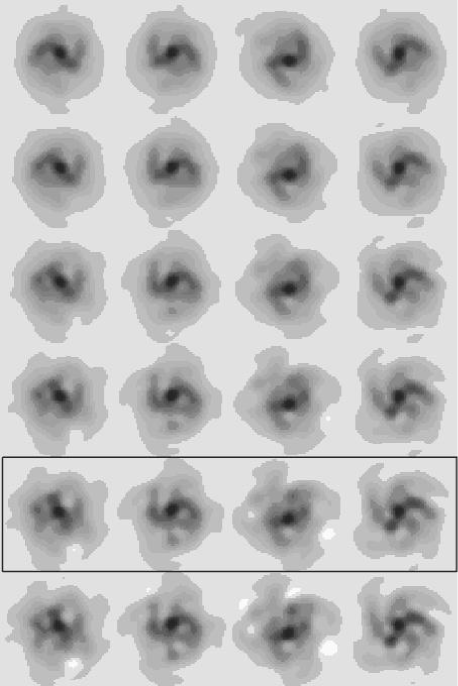
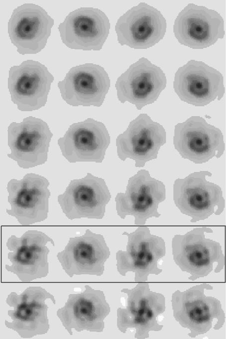
Figure 3: The effect of perturbing galaxy morphologies in shapelet space. Each image in the top row shows a real HDF galaxy, rotated by random angles. Its shapelet coefficients are incrementally perturbed in successive rows, although its overall flux is kept constant for the purpose of this plot. A degree of perturbation corresponding to our choice of the smoothing length $\lambda_{i}$ is shown inside the box: these images represent typical simulated galaxies. Perturbations larger than $\lambda_{i}$ produce objects which contain significantly negative pixel values. The left panel depicts a spiral galaxy; the right panel a more typical irregular form. The colour scale is logarithmic.

Many practical approaches have been devised to smooth discrete samplings of a multivariate PDF. Our main constraint in selecting one of these methods is the very high dimensionality of our data set. The median $n_{\rm max}$ required for objects in the HDF is 4. However, even with the efficient data compression that shapelets can afford, models of the highest S/N galaxies use values for $n_{\rm max}$ as high as 15. Adding object size and magnitude, this corresponds to 137 total coefficients, and this is therefore the maximum number of dimensions required.

To smooth and resample this dataset, we have chosen the Kernel smoothing method which is eloquently reviewed by Silverman (1986). Kernel smoothing can be considered as an alternative to using histograms. It avoids the ambiguity of binning and instead yields a smooth analytic curve. For 1-dimensional data, each sample data point is replaced by a smooth Gaussian kernel. To create a PDF, all the kernels can be summed and then normalised to integrate to unity. The width of these smoothing Gaussians still remains to be decided, but methods exist for optimising this factor. Each kernel can even be given a different width, calculated as a function of a quick local density estimate, in order to produce adaptive smoothing.

In data with more than one dimension, each sample point is replaced by a multivariate kernel. To help overcome the difficulties associated with the leaking of probability density into the wings of many-dimensional kernels, we replace the Gaussian with a more compact Epanechnikov kernel (Epanechnikov 1969),

$$K(\delta x_{i})=\left\{\begin{array}[]{cl}\frac{3}{4\lambda_{i}}\left(1-\left(\frac{\delta x_{i}}{\lambda_{i}}\right)^{2}\right)&{\mathrm{f}or}~{}-\lambda_{i}<\delta x_{i}<\lambda_{i}\\ 0&{\mathrm{e}lsewhere,}\end{array}\right.$$ (6)

where we have reformatted the shapelet coefficients of each HDF galaxy into a data vector $x_{i}$, and $\delta x_{i}$ are deviations in shapelet space from these real data points. In each case, $i$ is a coefficient index running from 1 to 137. $\lambda_{i}$ are smoothing widths which will be determined for each direction of our PDF space in §5.1. Isodensity contours of this kernel are multivariate ellipses whose axes are aligned with those of the co-ordinate axes (see figure 2). In general, they could be allowed to point in any direction (Sain 1999), but we do not find this to be necessary.

We implement an adaptive smoothing of our PDF by reparametrizing $a_{nm}$ as $\frac{a_{nm}}{a_{00}}$. Given a constant $\lambda_{i}$, this creates an effective smoothing kernel for each object of widths $\lambda_{i}^{\prime}=a_{00}\lambda_{i}$. This functional form is useful because the brighter HDF objects are less frequent, and are therefore more isolated in probability space. Since $a_{00}$ roughly correlates to total flux, we obtain a larger smoothing radius for brighter objects and better recover the underlying probability distribution. We will prove that this recipe does produce realistic morphologies in §6.

5 Image generation

5.1 Resampling the galaxy morphology PDF

Having recovered a realistic and analytic PDF of galaxy morphologies, we now wish to resample this distribution to generate brand new galaxy populations. The main advantage of the kernel smoothing approach now becomes apparent. Without resorting to costly numerical integration, Silverman (1986) $\S$6.4.1 presents a quick bootstrap method to generate a Monte-Carlo sample from a PDF constructed with $\delta$-functions smoothed by kernels $K$($\delta x$). We take the following steps to simultaneously smooth and resample the parameter space of HDF galaxies:

$$\left.\begin{array}[]{ll}Step~{}1:&{\mathrm{R}andomly~{}select~{}one~{}of~{}the~{}original~{}HDF}\\ &{\mathrm{g}alaxies,~{}uniformly~{}and~{}with~{}replacement.}\\ Step~{}2:&{\mathrm{G}enerate~{}a~{}small~{}perturbation~{}}\delta x_{i}~{}{\mathrm{f}rom}{}\\ &{\mathrm{t}he~{}probability~{}density~{}function~{}}K(\delta x_{i}).\\ Step~{}3:&{\mathrm{A}dd~{}}\delta x_{i}~{}{\mathrm{t}o~{}the~{}shapelet~{}coefficients~{}}x_{i}~{}{\mathrm{o}f}\\ &{\mathrm{t}he~{}HDF~{}galaxy.~{}This~{}simulates~{}a~{}new}\\ &{\mathrm{g}alaxy,~{}sampled~{}from~{}the~{}overall~{}PDF.}\end{array}\right\}$$ (14)

This approach is arrived at by simply regarding the PDF as a sum of small kernels rather than one overall function. Individually, these kernels are quick to compute; and the dimensionality of the PDF can even be lowered for faint objects that require fewer coefficients. The perturbations can be quickly sampled from an Epanechnikov kernel $K(\delta x)$ by generating three random numbers from a uniform probability distribution between $-\lambda_{i}$ and $\lambda_{i}$. If the first does not have the highest absolute value, take it and discard the rest; otherwise take the second. Iterating this procedure to generate sufficient objects for a simulated Hubble Deep Field requires only a few minutes on a 1GHz PC.

We must now decide how to choose the overall smoothing length $\lambda_{i}$. If $\lambda_{i}\equiv 0$, the kernel is a $\delta$-function and the original HDF objects are recovered exactly. This arrangement will create simulations of limited practical use, but in §6 they act as an intermediate test of the shapelet decomposition. As $\lambda_{i}\rightarrow\infty$, the coefficients for simulated galaxies become completely random and the objects become unrealistic. In this limit, since no positive-definite constraint is ever imposed in the shapelets formalism, we find that simulated objects exhibit undesirable holes of negative flux. Figure 3 shows realisations of how a typical galaxy from the HDF is altered by increasingly large perturbations to its shapelet coefficients, showing negative flux for large $\lambda_{i}$ perturbations.

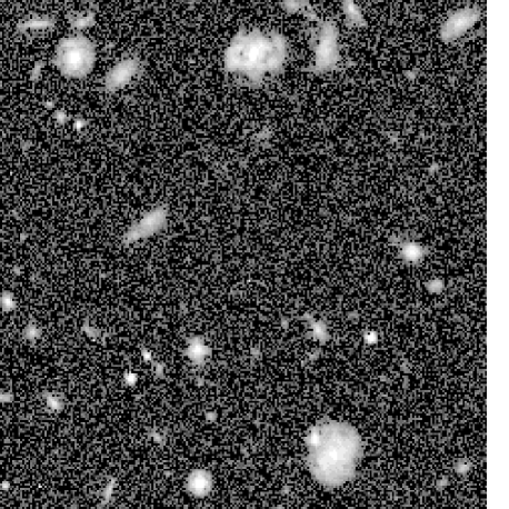
Figure 4: Sample HDF-depth simulated $I$-band image, 30″$\times$30″.

We therefore require a choice of $\lambda_{i}$ which is sufficiently large to produce new galaxies, yet sufficiently small to maintain realistic morphological properties. By measuring the minimum pixel values of many different galaxy realisations, we find suitable results if $\lambda_{phase}\la 15^{\circ}$ and $\lambda_{moduli}\la 4\times$[mean separation between nearest neighbours in that dimension]; beyond these values, negative holes rapidly appear. For the purposes of this paper, we therefore fix $\lambda_{i}$ to these limiting values. This still represents relatively weak smoothing, but the variety and realism of generated morphologies is pleasantly surprising: polar shapelets are indeed sufficiently close to the Principal Components of galaxy morphology that small perturbations in shapelet space correspond to reasonable and realistic changes within galaxy types. A quantitative demonstration of these remarkable results is presented in §6.

5.2 Scattering galaxies on the sky

A Monte Carlo population of genuinely new yet realistic objects has been extracted from the PDF of galaxy morphology. These galaxies are now allocated random orientations and locations on the sky, at a density of $700$ per arcmin². This constant has been calibrated to recover the same total number counts, after the addition of noise, as are measured in the HDFs (see §6.1). No attempt is made here to correctly model the 2-point correlation function of galaxy positions, or to include galaxy mergers beyond those sufficiently advanced to appear as one object in the input SExtractor catalogue.

The correct slope in the size and magnitude distributions are automatically ensured over a wide range of validity, since size and magnitude are intrinsic variables of the PDF (see the bottom-left panel of figure 2). However, it is important to consider the question of completeness in our simulations for very faint galaxies. A discrepancy could arise through either non-detections of faint HDF galaxies by SExtractor or non-convergence of their shapelet decompositions. The first effect is minimised by our choice of SExtractor parameters (see §2.1) and the second is shown in §2.2 to be under control. However, the number counts of galaxies at the very faint end ($I\lower 2.15277pt\hbox{$\;\buildrel>\over{\sim}\;$}29$) are also highly sensitive to the the precise background noise properties (see §5.3). For this reason, we choose not to consider galaxies fainter than $I=29$.

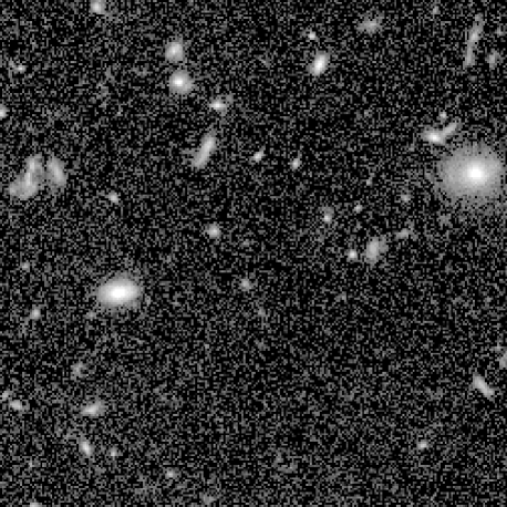
Figure 5: Section of the real HDF, with the same size and scale as figure 4.

At the bright end, we also expect the simulations to be incomplete, since the HDFs were intentionally chosen by STScI as areas containing few large, bright galaxies. In the future, we will extend our simulations in this respect by incorporating ‘Groth survey strip’ (Groth et al. 1994) and ACS galaxies into the object source catalogue. One could also compensate for any known incompleteness by preferentially selecting for under-represented galaxy types in step 1 of procedure (14).

5.3 Modelling telescope and observational effects

The shapelet models of galaxy images are actually analytic functions. These can quickly be convolved with a PSF that has also been decomposed into shapelets, using the matrix operation in Shapelets II $\S$3.1. Stars can also be included in an image, given a magnitude distribution, by repeatedly placing the shapelet model of the PSF in an image at the appropriate flux amplitude. All of these analytic objects are then integrated within square pixels of the same 0.0398″resolution as the DRIZZLEd Hubble Deep Field. Our images have a somewhat larger solid angle than the HDFs because the missing quarter from the WFPC ‘L’ is restored.

Observational noise can now be added, at a level appropriate to the desired exposure time. We have simply added photon counting noise (proportional to the square root of the raw pixel values), and Gaussian background noise (with an amplitude determined from the HDF itself). However, it would be easy to add a background level, cosmic rays and even instrumental distortions: the shearing for which could be performed conveniently in shapelet space before pixellisation. A further effect, not included in our simple model, is noise that is correlated between adjacent pixels. Aliasing occurs as a side-effect of the DRIZZLE algorithm, which recovers image resolution by stacking several dithered exposures. This aliasing can make it possible to detect slightly fainter objects and also introduces some spurious objects at very low S/N. The steep slope of the real number counts beyond $I=29$ exacerbates this problem, and we would not yet trust the noise model on our simulations for galaxies any fainter than this.

Final output is as a FITS image, a sample of which is displayed in figure 4. Larger images may be downloaded via anonymous ftp from the shapelets web page at http://www.ast.cam.ac.uk/$\sim$rjm/shapelets. Notice the wide range of galaxy morphologies and behaviours present in figure 4. In particular, features resembling spiral arms, dust lanes and resolved knots of star formation are present, together with various radial profile shapes. By eye, the simulated galaxies look very similar to those in a similarly-scaled section of the HDF itself, reproduced in figure 5. We will quantitatively examine whether our simulation effectively mimics the morphology distribution of HDF galaxies in the following section.

6 Statistical tests and results

We now demonstrate quantitatively that our simulated images are realistic, in the sense that commonly used morphology measures for our galaxies match the distributions of those for galaxies in the HDFs. First, we consider the number counts and size distributions, using photometry and size measures from SExtractor (Bertin & Arnouts 1996).These ought to be roughly consistent by construction, because they are closely related to two of the axes in our parameter space. Then we compare more detailed morphology measures, such as concentration (Bershady et al. 2000), asymmetry (Conselice et al. 2000a), clumpiness (Conselice et al. in preparation) and ellipticity. These are not automatically expected to match, because our shapelet-based PDF does not directly represent these quantities. Thus, a comparison between these properties for simulated and real data provides a rigorous and fair test of how realistic our simulations are.

6.1 Size and magnitude

In order to carry out these tests, we first apply the SExtractor object-finding and shape measurement package on the version 2 reductions of the HDF-N and HDF-S (Williams et al. 1996, 1998), together with a 6 arcmin² simulated image of the same depth. As an intermediate test, we also analyse a simulated image containing shapelet reconstructions of galaxies drawn from a PDF left as $\delta$-functions. These should be identical to the objects in the HDF and act as a test of the shapelets modelling procedure rather than the perturbations in shapelet space. In all four cases, approximately 320 galaxies brighter than $I\leq 29$ were detected per arcmin². For the galaxies only, we extracted observed magnitudes (MAG_BEST) and sizes (FWHM_IMAGE).

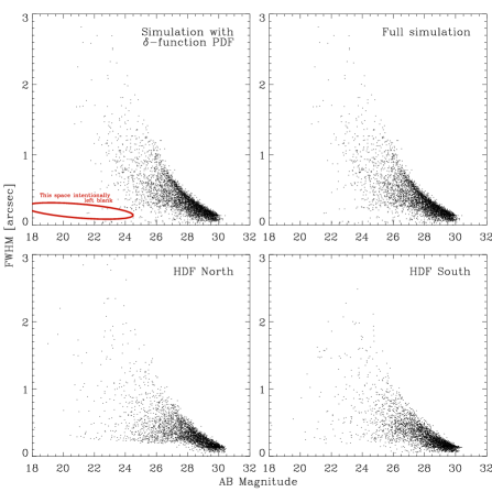
Figure 6: Size vs magnitude plane for 6 arcmin² $I$-band images to HDF depth, measured with SExtractor. Top-left panel: for a simulated image containing shapelet reconstructions of HDF galaxies (the PDF kept as $\delta$-functions). Top-right panel: for a simulated image with galaxies perturbed in shapelet space. Bottom panels: for real galaxies in the Hubble Deep Fields North and South, calculated using the same SExtractor input parameters as reference. The stellar locus is omitted from all panels.

Figure 6 compares the size vs magnitude distributions of the simulated images with those of the two HDFs, excluding the stars. Figure 7 then shows the galaxy number counts for real and simulated cases in more detail. These match well over six or more orders of magnitude, whether the simulations used a $\delta$-function PDF or the full version. Note, however, that the noise in the simulated images is not aliased in the same way as the DRIZZLE algorithm has caused the real data to become (see §5.3). The number counts beyond $I\sim 29$ are highly sensitive to background noise properties, and are indeed increased in the simulated image if we artificially smooth the noise. Clearly DRIZZLE is something that needs further attention in a future implementation.

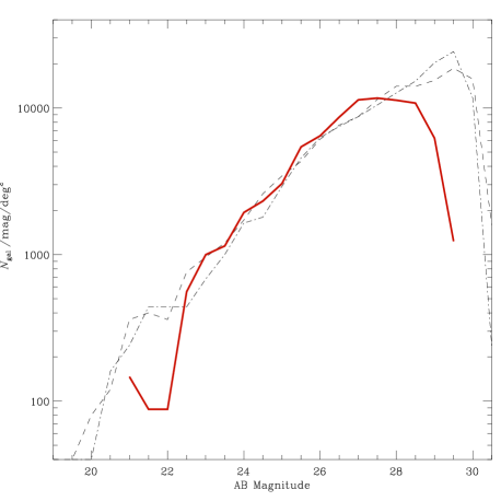
Figure 7: Number counts in simulated $I$-band images (solid red), normalised by area on the sky. Also shown are number counts for the Hubble Deep Field North (dot-dashed) and South (dashed).

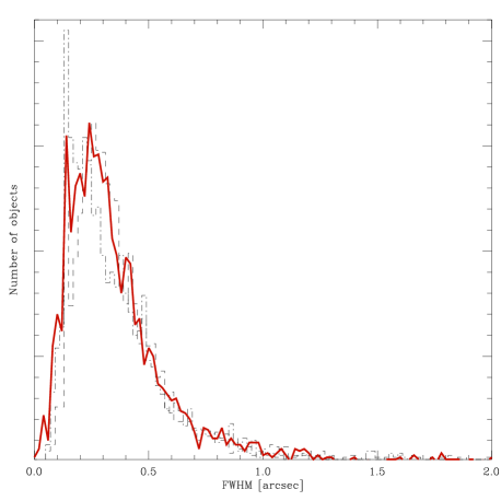
Figure 8: Size distribution of objects in a 6 arcmin² simulated image with limiting magnitude $I=29$ (solid red). Also shown are size distributions for the Hubble Deep Field North (dot-dashed) and South (dashed).

For the present purposes, we apply magnitude cuts and compare only the brighter objects, which are unaffected by such minor changes. These cuts are at levels determined by the stability of an individual diagnostic to noise. Figure 8 compares the size distribution of the simulated objects brighter than $I=29$ with those of the HDF galaxies, as found by SExtractor. We find that there is excellent agreement in the shape of this distribution: the median and standard deviation FWHM for real galaxies in the HDFs are 0.30″and 0.24″. For simulated objects, these figures are 0.31″and 0.23″. This agreement comes about partly (but not entirely) by construction. It was somewhat expected that our simulated images will closely match real data in terms of their magnitude and size distributions, but the final high precision is encouraging.

6.2 Galaxy morphology diagnostics

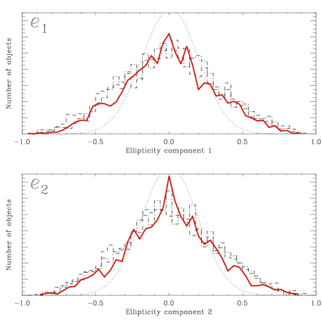
Figure 9: Ellipticity distribution, as defined in equations (15) and (16), of objects in 6 arcmin² simulated image with limiting magnitude $I=29$ (solid line). Also shown is the ellipticity distribution for the Hubble Deep Fields North (dot-dashed) & South (dashed), and a Gaussian with the same mean and rms (dotted).

We can more stringently test the reliability of our algorithm to reproduce properties of real galaxies by measuring morphological parameters which are entirely independent of shapelets. We apply a series of commonly used morphology diagnostics to two different realisations of the simulated images. A first version, containing unaltered shapelet models of HDF galaxies, tests the shapelet modelling process in isolation. A second simulated image, with galaxies drawn from the fully smoothed morphology PDF tests the fairness of these perturbations in shapelet space.

A first basic analysis is to determine the gross shape of galaxies, i.e. their ellipticities. The ellipticity of all the galaxies was obtained from SExtractor. Following a convention in weak lensing literature, we here define two independent components of ellipticity as

$$e_{1}\equiv\frac{{\mathrm{A}\_IMAGE}^{2}-{\mathrm{B}\_IMAGE}^{2}}{{\mathrm{A}\_IMAGE}^{2}+{\mathrm{B}\_IMAGE}^{2}}\cos(2\times{\mathrm{T}HETA\_IMAGE})$$ (15)

$$e_{2}\equiv\frac{{\mathrm{A}\_IMAGE}^{2}-{\mathrm{B}\_IMAGE}^{2}}{{\mathrm{A}\_IMAGE}^{2}+{\mathrm{B}\_IMAGE}^{2}}\sin(2\times{\mathrm{T}HETA\_IMAGE})$$ (16)

where A_IMAGE and B_IMAGE are the lengths of the major and minor axes of the ellipse, and THETA_IMAGE is the angle between the major axis and the horizontal (all parameters supplied by SExtractor). Figure 9 compares this ellipticity distribution of the real and fully simulated objects brighter than $I=29$. Again, these are in excellent agreement: with standard deviations in $e=\sqrt{e_{1}^{2}+e_{2}^{2}}$ of 0.64 for real data, 0.62 for simulated data using a $\delta$-function PDF and 0.62 for simulated data using the full PDF.

Figure 10: Concentration vs asymmetry, as defined in equations (17) and (18), for 6 arcmin² images with limiting magnitude $I$ = 26. Top-left panel: for a simulated $I$-band image containing shapelet reconstructions of HDF galaxies (the PDF kept as $\delta$-functions). Top-right panel: for a simulated image with galaxies perturbed in shapelet space. Bottom panels: for real galaxies in the Hubble Deep Fields North and South.

Figure 11: Concentration vs Petrosian radius, as defined in equation (17) and the text, for 6 arcmin² square images with limiting magnitude $I$ = 26. Panels are ordered as in Figure 10.

Figure 12: Asymmetry vs clumpiness, as defined in equations (18) and (19), for 6 arcmin² square images with limiting magnitude $I$ = 25. Panels are ordered as in Figure 10.

The four images have also been passed through the model-independent morphology software developed by Conselice et al. (2002a), Bershady et al. (2000) and Conselice (2003), in order to measure the concentrations ($C$), asymmetries ($A$) and clumpiness ($S$) values of the real and simulated galaxies. We first describe how these three quantities are calculated, and then compare the distributions obtained for these measures from real data and simulations. These ‘$CAS$’ parameters are very informative, as all nearby galaxy types (ellipticals, spirals, dwarfs, etc.) fall in distinct regions of $CAS$ space (Conselice 2003). These parameters thus capture most of the variation in galaxy structures and have frequently been used for quantitative morphology classification.

The concentration index, $C$, is defined in terms of the ratio of the radii containing 80% ($r_{80}$) and 20% ($r_{20}$) of the object’s total flux:

$$C\equiv 5\times\log\left(\frac{r_{80}}{r_{20}}\right)~{}.$$ (17)

For the total flux, we use the flux within an aperture $1.5$ times the size of the Petrosian radius at $\eta=0.2$ (Bershady et al. 2000). The $\eta$ parameter is defined as the ratio of the surface brightness at a radius divided by the surface brightness integrated within the radius, such that at the centre of a galaxy, $\eta=1$ and at the very edge of a galaxy (where its surface brightness is 0), $\eta=0$.

Typical values of $C$ for real galaxies range from approximately 2 to 6. Galaxies with $C>4$ are usually ellipticals or spheroidal systems: a galaxy with an $r^{1/4}$ profile has $C=5.2$. A purely exponential disc galaxy has $C=2.7$ (Bershady et al. 2000). Objects with lower light concentrations are shown by Graham et al. (2001) to be systems with low central surface brightnesses and often low internal velocity dispersions. Low concentration values are also found for dwarf galaxies (e.g. Conselice et al. 2002). The concentration index thus correlates, within some scatter, with the total mass of a galaxy.

The asymmetry index used in this paper (called $A_{180}$ in Conselice et al. 2000a,b) is calculated by rotating an image by $180\degr$ and subtracting the it from the original. Then we evaluate

$$A\equiv\min\left[\frac{\sum|I_{x,y}-I_{x,y}^{180}|}{\sum|I_{x,y}|}\right]-\min\left[\frac{\sum|B_{x,y}-B_{x,y}^{180}|}{\sum|I_{x,y}|}\right],$$ (18)

where $I_{x,y}$ is the galaxy surface brightness in the $(x,y)$ pixel of the image, $B_{x,y}$ the sky background in the same pixel, and superscripts denote rotations. Sums are over all pixels within the same $\eta=0.2$ Petrosian radius from which the total light measurement is made. Minimisation is then over different choices of the centre of rotation (see Conselice et al. 2000a).

The asymmetry index is sensitive to any physical processes in a galaxy that produce asymmetries in light distributions, such as star-formation, galaxy interactions/mergers, and projection effects such as dust lanes. There is a general correlation between the asymmetry value and the ($B-V$) colour (Conselice et al. 2000a). Since most galaxies are not edge-on systems, star formation and galaxy interactions/mergers are the dominant effects that produce asymmetries in real galaxies. These two effects can often be distinguished, however. Systems with asymmetries $A>0.35$ are generally created by interactions or mergers (Conselice 2003, Conselice et al. 2003). However, other merger events can have more modest asymmetry values. From this and more detailed studies of the asymmetry index, it has been concluded that $A$ is most sensitive to bulk structures in galaxies (Conselice 2003).

The clumpiness parameter, $S$, is a measure of the high-spatial frequency component of galaxies. It is calculated by smoothing a galaxy’s image with a smoothing length $\sigma$, then subtracting this smoothed version $I_{x,y}^{\sigma}$ from the original image. This leaves a residual map containing only those features with a high-spatial frequency. Summation is again performed over pixels within the $\eta=0.2$ Petrosian radius, although those from the central cusp are ignored. Also including a correction for the background B_x,y, the clumpiness is then defined as

$$S\equiv 10\times\frac{\sum_{xy}|I_{x,y}-I_{x,y}^{\sigma}|-\sum_{xy}|B_{x,y}-B_{x,y}^{\sigma}|}{\sum_{xy}I_{x,y}}~{}.$$ (19)

The clumpiness index is sensitive to the instantaneous rate of star formation, and correlates very well with H$\alpha$ equivalent widths; it also correlates to a lesser degree with broad-band colors (Conselice 2003). Other details of its calculation and properties are discussed in detail in Conselice (2003).

We also use the Petrosian radius $R$ (Petrosian 1976) to characterise the galaxies, defined as the position where $\eta=0.2$. The Petrosian radius is found to be a better index than the SExtractor FWHM radius for determining morphological sizes, as SExtractor radii are based on isophotal thresholds which will represent different physical distances from the galactic centre depending on the distance to the galaxy. Because $\eta$ is a ratio of surface brightnesses in a given galaxy, the run of $\eta$ with $r$ in a galaxy is immune to many such types of systematic effects (Sandage & Perlmutter 1990) and Petrosian radii are found to be a stable tool for deriving morphological parameters independent of distance (Bershady et al. 2000).

We are now in a position to compare the measurements for $C$, $A$, $S$ and $R$ for real and simulated images. Projections from this morphological parameter space for real and simulated data are displayed in figures 10–12, and relevant statistics are compiled in table 1.

	HDF-N	HDF-S	Simulation with	Full
			$\delta$-function PDF	simulation
$\langle C\rangle$	3.11	3.13	3.03	3.07
rms $C$	0.39	0.40	0.44	0.42
$\langle A\rangle$	0.18	0.17	0.19	0.07
rms $A$	0.20	0.22	0.27	0.25
$\langle S\rangle$	0.23	0.28	0.27	0.08
rms $S$	0.28	0.28	0.15	0.19
rms $e$	0.64	0.64	0.62	0.62

Table 1: Galaxy morphology statistics. The first two columns show results for real objects, taken from the Hubble Deep Fields. Compare this with objects in simulations created using a $\delta$-function PDF or the full shapelet-morphing procedure.

As can be seen from the scatter in the plots, the agreement between simulations and real data is rather good: we are very pleased by the encouraging results. The matching distributions of the concentration parameter puts to rest one criticism frequently levelled at shapelets (see §3), that a truncated Gaussian-Laguerre expansion may not stretch far enough spatially to capture the extended wings of typical astronomical objects. Clearly our algorithm sets $n_{\rm max}$ high enough to avoid this problem while still modelling the HDF galaxies using only a few coefficients.

The final population of simulated galaxies does contain asymmetry values lower than those in the real data, although the distributions agree within 1$\sigma$. This slight discrepancy is neither due to deficiencies in the shapelet modelling procedure, nor to the increased clustering of galaxies at short separations in real data, because it is absent from the simulation created with a $\delta$-function PDF. Decreased object asymmetry must therefore be a by-product of the PDF smoothing. There is no obvious a priori reason why this should happen. Even $m$ states are symmetric and odd $m$ states anti-symmetric, so if the absolute values of all coefficients are randomly changed by the same amount, the overall symmetry of the object should stay constant. However, our nearest-neighbour prescription from §5.1 results in an average smoothing length across typical even $m$ states, and particularly the $m=0$ states, of approximately twice that for odd $m$ states. This may simply be because the first state is even, and the smoothing length tends to get shorter as $n$ increases. A more sophisticated adaptive smoothing method might be found to prevent this effect, but we have not pursued that idea here. We note the asymmetry discrepancy, but note also that it is relatively small.

The behaviour of the clumpiness parameter is also reasonable. Truncation in shapelet modelling smooths galaxies slightly, and thus removes the tail of objects with very high $S$. Morphing in shapelet space apparently acts to then smooth some of the galaxies further. This is peculiar because, if anything, the galaxies in figure 3 appear by eye to become more clumpy as the smoothing length is increased. Overall, the agreement of the simulated distributions with real data is remarkably consistent with the field-to-field variation between the two HDFs. Indeed, clumpiness is a rather unstable statistic to measure. For example, even the slight rise in mean clumpiness for the $\delta$-function simulation might be significant: especially since it is apparent despite the missing tail at high $S$. It is possible that the increase is caused by residual artefacts in the shapelet models, but more plausibly because the noise in our simulated images is not correlated between adjacent pixels. The HDFs themselves have been DRIZZLEd in order to achieve their high resolution, a process which also aliases the image. As a simple approximation to this effect, we have tried smoothing the noise slightly in our simulations, by a top hat kernel 3 pixels wide. This process does indeed remove the slight disparity observed in the simulated clumpiness distribution, but simultaneously creates many false detections of faint, circular objects from the noise at the magnitude limit around $I\geq 29$.

Therefore we conclude that our shapelet simulations obtain similar morphology distributions to those found in real data. This is most encouraging as these were not arranged by construction, and the level of realism seen here is a strong vindication of the shapelet modelling of galaxies. Perturbing shapelet parameters to create new galaxies can introduce a few minor deviations, but these are small compared to natural variation between objects, and are well understood and quantified. We can therefore use shapelets as a tool for investigating galaxy morphology and for creating realistic simulated images.

7 Comparison to other methods

There have been many packages in the literature which simulate astronomical observations, including Skymaker (see Erben et al. 2001) and artdata in IRAF (Tody 1993). These typically parametrize galaxy shapes using simple physical models such as ellipses with de Vaucouleurs or exponential profiles. The smooth variation allowed for these parameters enables them to generate an unlimited number of unique simulated galaxies. These methods are particularly valuable for simulating images from ground-based telescopes. Unfortunately, deep images from HST contain galaxies with resolved features more complex than these analytical models, so such simulations are useful in only a limited regime.

This was realised by Bouwens, Broadhurst & Silk (1998), who designed simulations to investigate the evolution of galaxy morphology in the HDF. Indeed, their work succeeds in ruling out pure luminosity evolution of galaxies: which precisely demonstrates the need for deep image simulations to contain more irregular and asymmetric morphologies. Their method repeatedly places the few brightest HDF galaxies onto a simulated image, and is similar to that which ours would have been, had we left the PDF as an (unsmoothed) sum of $\delta$-functions. Some physics can be added to rescale and redshift these few sources, but it remains a very small population from which to simulate a large imaging survey, and containing members drawn exclusively from the local universe. Creating realistic images was not the intention of Bouwens, Broadhurst & Silk (1998) and, for our objectives, their method would require the addition of more physics (e.g. galaxy evolution, star formation histories, redshift distributions, etc.).

Our technique attempts to capture the best aspects of both methods, by defining a smooth parameter space that can yield an unlimited number of unique galaxies, but also contains a rich diversity of their morphologies (potentially any morphology, in fact, since the set of shapelet basis functions is complete). Since the parameter space is populated via statistical rather than physical arguments, it is the many tests to which we have subjected our simulated images that demonstrate the validity of our method. We find a regime spanning six orders of magnitude in luminosity where our simulations are valid, and their statistical properties match those of real data. This ability to produce simulated images containing galaxies with realistic morphologies is a significant advance.

8 Conclusions

We have presented a method for generating simulated deep sky images of an arbitrarily large survey area, as might be observed with extended observations with the Hubble Space Telescope. These simulated images are populated with all morphological types of galaxies, based upon those in the Hubble Deep Fields.

The simulated galaxies are drawn from a multi-variate distribution of realistic morphologies, described using the shapelet formalism (Refregier 2003). In order to generate this morphology distribution, we decompose all HDF galaxies into shapelet components using least-squares fitting. We optimise this decomposition by finding the scale length $\beta$ and number of modes $n_{\rm max}$ which produces a best shapelet coefficient fit to each galaxy. The resulting coefficients of HDF galaxies form a cloud of points in shapelet space; these points are replaced by smooth kernels in order to recover the underlying probability distribution of real galaxy morphologies. The smooth distribution is then resampled, using an unbiased Monte-Carlo technique, to obtain new galaxies.

We place these simulated galaxies onto HDF-sized images, simultaneously including effects such as PSF, pixellisation, photon shot noise and Gaussian background noise. The level of detail in the resulting simulated galaxies includes features such as realistic radial profiles, spiral arms, dust lanes and resolved knots of star formation.

We have noted that the global morphological properties of the simulated galaxy population must match those of real galaxies if our simulations are to be useful. We have demonstrated that this is the case by comparing various morphology diagnostics in simulated and real galaxies, including number counts as a function of magnitude, the size distribution, ellipticity distribution, and concentration, asymmetry and clumpiness indices. A test involving purely the shapelet decomposition and reproduction of the HDF galaxies preserves all of these statistics with high precision, and we conclude that a shapelet decomposition can successfully capture the morphological properties of all galaxy types. A few slight discrepancies are introduced to the statistics by perturbing their shapelet coefficients (or smoothing the morphology distribution) to manufacture genuinely new galaxy shapes. However, these differences are small compared to even the natural variations between objects. Several minor effects have been well quantified by our various tests, and their causes understood for correction in future implementations.

An important application for our simulated images is presented in Massey et al. (2003), where they are used to predict the sensitivity to weak gravitational lensing of the proposed SNAP satellite. However, the simulations presented here are in no way specific to gravitational lensing, and may be used for testing image analysis in various branches of astronomy. Further simulated images and catalogues are available from the authors.

A useful extension to this work will be to include ‘Groth survey strip’ (Groth et al. 1994) galaxies and ACS data when constructing the morphology probability distribution. This will provide future simulations with a more extensive sample of large, bright galaxies, improving the fidelity of the simulations in this region of parameter space. A method is also in development to generate multi-colour simulated images using several HDF passbands and photometric redshifts. A by-product of this work is a complete morphological catalogue of all the HDF galaxies in shapelet space. This catalogue will be used in a future paper on the automated morphological classification of galaxies at high redshift.

References

- [1] Abraham R. et al. 1996, ApJS, 107, 1
- [2] Bacon D., Refregier A., Clowe D. & Ellis R. 2001, MNRAS, 325, 1065
- [3] Bartelmann M. & Schneider P. 2001, Physics Reports, 340, 291
- [4] Bernstein G. & Jarvis M. 2002, AJ, 123, 583
- [5] Bershady M., Jangren A. & Conselice C. 2000, AJ, 119, 2645
- [6] Bertin E. & Arnouts S. 1996, A&AS, 117, 393
- [7] Blinnikov S. & Moessner R. 1998, A&AS, 130, 193
- [8] Boas M. 1983, “Mathematical Methods in the Physical Sciences”, Wiley.
- [9] Bouwens R., Broadhurst T. & Silk J. 1998a, ApJ, 506, 557
- [10] Bouwens R., Broadhurst T. & Silk J. 1998b, ApJ, 506, 579
- [11] Conselice C., Bershady M. & Jangren A. 2000a, ApJ, 529, 886
- [12] Conselice C., Bershady M. & Gallagher J. 2000b, A&A, 354, 21L
- [13] Conselice C., Gallagher J. & Wyse R. 2002, AJ, 123, 2246
- [14] Conselice C. 2003, ApJS, in press, astro-ph/0303065
- [15] Conselice C., Bershady M., Dickinson M. & Papovich, C. 2003, AJ, 126, 1183
- [16] Driver S. 1999 in Looking Deep in the Southern Sky, eds F. Morganti and W. Couch. Berlin: Springer-Verlag p.280
- [17] Epanechnikov, V. 1969, “Nonparametric Estimation of a Multivariate Probability Density”, Theory of Probability and Its Applications, 14, 153
- [18] Erben T., van Waerbeke L., Bertin E., Mellier Y. & Schneider P. 2001, A&A, 366, 717
- [19] Francis P. & Wills B. 1999, in “Quasars and Cosmology”, A.S.P. Conference Series 1999, eds. G. Ferland, J. Baldwin (San Francisco: ASP)
- [20] Fruchter A. & Hook R. 2002, PASP, 114, 144
- [21] Gerhard O. 1993, MNRAS, 265, 213
- [22] Groth E. et al. 1994, BAAS, 185, 5309
- [23] Hubble E. 1926, ApJ, 64, 321
- [24] Kaiser N., Squires G. & Broadhurst T. 1995, ApJ, 449, 460
- [25] Krist J. 1995, ADASS IV, A.S.P. Conference Series, Vol. 349
- [26] Krist J., & Hook R. 1997, The Tiny Tim User’s Guide (Baltimore: STScI)
- [27] Lupton R. 1993, Statistics in Theory and Practice (Princeton U. Press: Princeton)
- [28] Marleau F. & Simard L. 1998, ApJ, 507, 585
- [29] Marshall P. 2003, in preparation
- [30] Massey R. et al. 2003, AJ, submitted, astro-ph/0304418
- [31] Mellier Y. 1999, ARA&A, 37, 127
- [32] Meyer Y. 1993, “Wavelets: Algorithms and Applications”, Society for Industrial and Applied Mathematics, Philadelphia
- [33] Odewahn S., Windhorst R., Driver S. & Keel W. 1996, ApJL, 472, 13
- [34] Peng C., Ho L., Impey C. & Rix H.-W. 2002, AJ in press.
- [35] Petrosian V. 1976, ApJ, 209, 1L
- [36] Piña R. & Puetter R. 1993, P.A.S.P., 105, 630
- [37] Ratnatunga K., Griffiths R. & Ostrander E. 1999, AJ, 118, 86
- [38] Refregier A. 2003, MNRAS, 338, 35
- [39] Refregier A. & Bacon, D. 2003, MNRAS, 338, 48
- [40] Rhodes J., Refregier A. & Groth E. 2001, ApJ, 552, 85
- [41] Sandage A. 1961, “The Hubble Atlas of Galaxies” (Carnegie Inst. Washington Publ. 618) (Washington: Carnegie Inst.)
- [42] Sain S. 1999, “Multivariate Locally Adaptive Density Estimation”, Technical Report, Department of Statistical Science, Southern Methodist University
- [43] Sérsic J. 1968, “Atlas de Galaxias Australes” (Cordoba: Obs. Astronomico)
- [44] Silverman B. 1986, “Density Estimation for Statistics” and Data Analysis (Chapman and Hall, London)
- [45] Simard L. 1998, ADASS VII, A.S.P. Conference Series, Vol. 145, 108
- [46] Stark J.-L., Pantin E. & Murtagh F. 2002, PASP, 114, 1051
- [47] Tody D. 1993, “IRAF in the Nineties” in ADASS II, A.S.P. Conference Series, Vol 52, eds. R. Hanisch, R. Brissenden, & J. Barnes, 173
- [48] Van der Marel R. & Franx M. 1993, ApJ, 407, 525
- [49] Van der Marel R. et al. 1994, MNRAS, 268, 521
- [50] de Vaucouleurs G. 1959, Hand. Physik, 53, 275
- [51] Williams R. et al. 1996, AJ 112, 1335
- [52] Williams R. et al. 1998, A&AS, 193, 7501
- [53] York D. 2000, AJ, 120, 1579