THE MASS PROFILE OF GALAXY CLUSTERS
OUT TO $\sim 2r_{200}$

Abstract

We use the public release of $\simeq 100,000$ galaxies of the Two Degree Field Galaxy Redshift Survey (2dFGRS) to analyze the internal dynamics of galaxy clusters. We select 43 non-interacting clusters which are adequately sampled in the 2dFGRS public release. Members of these clusters are selected out to $\sim 2$ virial radii. We build an ensemble cluster by stacking together the 43 clusters, after appropriate scaling of their galaxy velocities and clustercentric distances. We solve the Jeans equation for the hydrostatic equilibrium for the member galaxies within the virial radius of the ensemble cluster, assuming isotropic orbits. We constrain the cluster mass profile within the virial radius by exploring parameterized models for the cluster mass-density profile. We find that both cuspy profiles and profiles with a core are acceptable. In particular, the concentration parameter of the best fit NFW model is as predicted from numerical simulations in a $\Lambda$CDM cosmology. Density profiles with very large core-radii are ruled out. Beyond the virial radius, dynamical equilibrium cannot be taken for granted, and the Jeans equation may not be applicable. In order to extend our dynamical analysis out to $\sim 2$ virial radii, we rely upon the method which uses the amplitude of caustics in the space of galaxy clustercentric distances and velocities. We find very good agreement between the mass profile determined with the caustic method and the extrapolation to $\sim 2$ virial radii of the best-fit mass profile determined by the Jeans analysis in the virialized inner region. We determine the mass-to-number density profile, and find it is fully consistent with a constant within the virial radius. The mass-to-number density profile is however inconsistent with a constant when the full radial range from 0 to $\sim 2$ virial radii is considered, unless the sample used to determine the number density profile is restricted to the early-type galaxies.

1 INTRODUCTION

The determination of cluster masses has a long story (see, e.g. Biviano, 2002, for a review). It dates back to Zwicky (1933, 1937)’s and Smith (1936)’s preliminary estimates of the masses of the Coma and the Virgo cluster. These early estimates were based on the virial theorem, using galaxies as unbiased tracers of the cluster potential (i.e. the light traces mass hypothesis). The & White (1986) and Merritt (1987) were among the first to point out that cluster masses were in fact poorly known, since relaxing the light traces mass assumption widens the range of allowed mass models considerably. However, the limited amount of redshift data made it very difficult, if not impossible, to constrain the relative distributions of cluster mass and cluster light.

With the advent of multi-object spectroscopy, a large number of redshifts for cluster galaxies became available. In particular, the two main catalogs of redshifts of cluster galaxies became available, viz. the ESO Nearby Abell Cluster Survey (ENACS, Katgert et al., 1996, 1998), and the Canadian Network for Observational Cosmology (CNOC, Yee et al., 1996; Ellingson et al., 1998). Moreover, field galaxy surveys also contributed to increase the number of redshifts for cluster galaxies, in particular, the Century Survey (Wegner et al., 2001), and the Two Degree Field Galaxy Redshift Survey (2dFGRS, Colless et al., 2001; De Propris et al., 2002, hereafter DP02).

These new data-bases prompted new more detailed investigations in the issue of the cluster mass determination. With a significant number of galaxy redshifts per cluster, it became possible to determine the cluster mass profile by solving the Jeans equation (e.g., Binney & Tremaine, 1987) for the equilibrium of member galaxies in the cluster gravitational potential. Often, several cluster samples have been combined to improve the statistics, by making the implicit assumption of cluster homology.

From the analysis of $\sim 1000$ galaxies in the CNOC clusters, combined to form a single cluster, Carlberg et al. (1997a) concluded that galaxies trace the mass to within $\pm 30$%, and that the cluster mass profile is well described by a Navarro, Frenk & White (1997, NFW hereafter) profile, or by a Hernquist (1990) profile. Their results have substantially been confirmed by the more detailed analysis of van der Marel et al. (2000, hereafter vdM00). vdM00 found that the mass-to-light ratio is almost independent of radius, and the NFW profile is an adequate fit to the data, but other density profiles are equally acceptable, depending on the orbital anisotropy of cluster galaxies. Carlberg et al. (2001) have recently applied the technique of Carlberg et al. (1997a) to a sample of $\sim 700$ galaxies in $\sim 200$ groups from the CNOC2. They found a strongly increasing mass-to-light ratio with radius, a result at variance with that found by Mahdavi et al. (1999). A detailed analysis of the mass and anisotropy profiles of clusters from ENACS is ongoing (Katgert, Biviano & Mazure, in preparation).

A new technique for the determination of cluster mass profiles has recently been introduced by Diaferio & Geller (1997) and Diaferio (1999, hereafter D99). It is based on the determination of the amplitude of the caustics in the space of velocities and clustercentric radii. Applications of this technique include Geller, Diaferio & Kurtz (1999)’s and Rines et al. (2001)’s determination of the Coma cluster mass profile out to 14 $h^{-1}$ Mpc, Rines et al. (2000)’s determination of the mass profile of Abell 576 out to 6 $h^{-1}$ Mpc, and Reisenegger et al. (2000)’s determination of the mass of the Shapley supercluster. The NFW profile was found to provide a consistent fit to the mass profiles. Interestingly, Rines et al. (2000) found a decreasing mass-to-light profile in Abell 576 while Rines et al. (2001) found a constant mass-to-light profile in Coma.

From a theoretical point of view, both decreasing and increasing mass-to-light profiles have been predicted. A decreasing mass-to-light profile could result from the tidal stripping of galaxy halos in the cluster centers (Mamon, 2000). An increasing mass-to-light profile could instead result from the combined effects of dynamical friction and galaxy merging (Fusco-Femiano & Menci, 1998). In general, galaxies are unlikely to be distributed exactly like the mass, if anything because different galaxy populations have different distributions (e.g., Biviano et al., 2002).

In this paper we determine the mass profile of an ensemble cluster built from the combined data of 43 clusters extracted from the 2dFGRS (Colless et al., 2001), using the techniques described by vdM00 and Diaferio & Geller (1997, see also D99). Since the 2dFGRS is a field survey, only a small fraction of the 2dFGRS galaxies are cluster members. Our final sample contains 1345 cluster members only, a number comparable to that of cluster members in the CNOC and smaller than that of cluster members in the ENACS. The main advantage of using the 2dFGRS for the determination of the cluster mass profile is the possibility of sampling the cluster dynamics to a large distance from the cluster center.

This paper is organized as follows. In § 2 we describe the data sample, how we assign the cluster membership and how we combine the 43 cluster data-sets into a single ensemble cluster. In § 3 we determine the ensemble cluster mass profile. In § 4 we use this mass profile to determine the mass-to-number density profile. In § 5 we discuss our results and compare them with previous determinations of cluster mass and mass-to-light profiles. Finally, in § 6 we present a summary of our results. A Hubble constant of 100 $h$ km s${}^{-1}\;$Mpc^-1 is used throughout.

2 THE DATA SAMPLE

The data sample we use is the 2dFGRS public release version of June, 30^th, 2001. It contains $\sim 100,000$ redshifts and spectral types as well as $b_{\mbox{J}}$ photometry for $\sim 460,000$ objects. The $b_{\mbox{J}}$ magnitudes are extinction-corrected total magnitudes derived from updated versions of the original APM (Automated Plate Measuring machine) scans (see Colless et al., 2001; Norberg et al., 2001). The target galaxies for the 2dFGRS were selected to have $b_{\mbox{J}}\leq 19.45$. Within the 2dFGRS public release, we only consider those galaxies in the fields of galaxy clusters. Galaxy clusters have been identified in the 2dFGRS by DP02, via a cross-correlation of the 2dFGRS with the cluster catalogs of Abell, Corwin, & Olowin (1989, hereafter, ACO), of Lumsden et al. (1992, the Edinburgh-Durham Cluster Catalogue, EDCC) and of Dalton et al. (1997, the APM cluster catalog). From DP02’s sample we exclude those clusters whose central regions are not evenly sampled in the 2dFGRS public release, and those which, according to the authors themselves, have less than 20 members with redshifts in the 2dFGRS. Of course, we also get rid of double entries in DP02’s list (such as, e.g., APM 309 which corresponds to ACO 3062). We are thus left with 91 clusters.

Following Carlberg et al. (1997a) we define $r_{u}\equiv\sqrt{3}\,\sigma_{p}/[10H(z)]\simeq r_{200}$, the radius at which the mean interior overdensity is 200 times the critical density (in a $\Omega_{0}=1$ Universe), usually called the ’virial radius’. As a first estimate of the clusters projected velocity dispersions along the line-of-sight, $\sigma_{p}$’s, we use DP02’s values.

To these 91 clusters, we apply the selection procedure of cluster members of Fadda et al. (1996) and Girardi et al. (1998). First, we apply Pisani (1993)’s one-dimensional algorithm based on the adaptive kernel technique (see also Appendix A of Girardi et al. 1996). The adaptive kernel technique is a nonparametric method for the evaluation of the density probability function underlying an observational discrete data set. The method returns a list of all density peaks detected, as well as their probabilities, and the objects associated to each peak. We apply this method to the velocity distribution of all galaxies projected within $2r_{u}$ of each cluster center. We select as significant those peaks with $\geq 98$% probability. When adjacent peaks have 20% or more of their objects in common, we join them together if they are closer in velocity than 1500 km s^-1. When one peak is closer than 1500 km s${}^{-1}\;$to two other peaks, themselves separated by more than 1500 km s^-1, we join the central peak to the one which is closest, and leave the third peak separate.

Quite often, several significant density peaks are found in a single cluster region. Among the significant peaks, we choose that one which is closest to the mean cluster velocity, as given by DP02. In this way we avoid possible mis-identifications, since sometimes the search region around each cluster (a circle of $2r_{u}$ radius) is wide enough to contain another cluster.

We identify 75 clusters with a significant density peak in the velocity space and at least 20 galaxies associated to that peak. In one case (ACO-S1155), no significant peak is found, and in another 15 cases, there are less than 20 galaxies in the peak corresponding to the cluster. These 16 clusters are excluded from our sample.

We re-define the centers of the 75 clusters. We define the new cluster center as the position of the highest density peak found with a two-dimensional adaptive kernel technique. In order to avoid mis-identifications, we only use galaxies less distant than 0.5 $h^{-1}$ Mpc  from the old cluster center listed by DP02. Using these new center determinations, we apply the ’shifting-gap’ method (Fadda et al., 1996) to get rid of the remaining interlopers. The shifting-gap method makes use of both galaxy velocities and clustercentric distances. Galaxies are sorted in order of increasing distance from their cluster centers. Among samples of galaxies in (overlapping and shifting) bins of 0.4 $h^{-1}$ Mpc  from the cluster center (or wide enough to contain $\geq 15$ galaxies each), gaps $\geq 1000$ km s${}^{-1}\;$are identified in the galaxy velocity distribution. These gaps define the edges of the galaxy velocity distribution. Outliers from this distribution are flagged as interlopers.

Having excluded the interlopers, we make a new estimate of the cluster mean velocities, $\overline{v}$’s, and velocity dispersions, $\sigma_{p}$’s, (and hence $r_{u}$’s). The velocity moments are estimated with the robust methods of Beers, Flynn, & Gebhardt (1990, see also ). Velocity dispersions are corrected for the velocity errors and moved to the cluster rest-frames (Danese et al., 1980). These new $\overline{v}$, $\sigma_{p}$ and $r_{u}$ estimates are the starting values for an iterative procedure. We consider only the cluster members within a distance $\leq r_{u}$ from the cluster center to recalculate $\overline{v}$ and $\sigma_{p}$. If the difference between the new estimate of $\sigma_{p}$ and the previous one is $\leq 10$%, the procedure is halted. Otherwise, we iterate, by recalculating $\overline{v}$ and $\sigma_{p}$ on the members within a distance of $\leq r_{u}$ from the cluster center, where the new value of $r_{u}$ is used. With this iterative procedure, we eliminate 7 of the initial 75 clusters, because they are left with less than 5 members within $r_{u}$ at any of the iteration steps.

With the new center and $r_{u}$ determinations, we then iterate the adaptive-kernel procedure and the shifting-gap method for the selection of cluster members. This time, we extend the search region to $3r_{u}$, in order to ensure that we will be covering a region of at least $2r_{u}$ radius when the final definitive estimate of $r_{u}$ is done. On the selected galaxies we re-determine $\overline{v}$ and $\sigma_{p}$ via the iterative procedure described above. We are left with a sample of 67 clusters, after eliminating one because it contains less than 5 members within $r_{u}$.

In order to determine the mass profile of galaxy clusters to sufficiently large distances, it is wise to exclude interacting clusters, whose dynamics is difficult to model. Say $\overline{v_{i}}$, $\sigma_{i}$, and $r_{u,i}$ are, respectively, the mean velocity, velocity dispersion, and virial radius of cluster $i$, and $R_{i,j}$ is the projected distance between the centers of clusters $i$ and $j$; we say cluster $i$ and cluster $j$ are ’interacting’ if the following two conditions apply:

$$\mid\overline{v_{i}}-\overline{v_{j}}\mid<3(\sigma_{i}+\sigma_{j})\\$$ (1)

$$R_{i,j}<2(r_{u,i}+r_{u,j}).$$ (2)

We eliminate 24 interacting clusters, and we are thus left with a sample of 43 reasonably isolated clusters.

Before we can construct azimuthally averaged profiles, we must verify that the circular region of $2r_{u}$ radius around each cluster center is fully covered in the 2dFGRS public release data sample. This is indeed the case for all the clusters in our sample, except two, APM 715 and ACO 892. For these two clusters we define an angular sector which excludes the region not covered in the 2dFGRS public release data sample, and we consider only the galaxies within this sector.

Figure 1: Distribution of galaxies of the ensemble cluster in the space of normalized clustercentric distances and velocities. Top panel: large dots indicate cluster members. Bottom panel: large dots indicate the 642 cluster members, late-type spirals excluded, within $R\leq r_{u}$, on which the Jeans analysis is based. The vertical dashed line indicates the $R=r_{u}$ limit beyond which the cluster membership assignment is less reliable.

Using a two-dimensional Kolmogorov-Smirnov test (e.g. Fasano & Franceschini, 1987) we also verify that the spatial distributions of galaxies with and without redshifts are not significantly different, at least out to $2r_{u}$. There are only four clusters for which there is a marginal ($\geq 90$%) evidence of a difference: ACO 957, ACO 1750, ACO 2734, EDCC 153. For these clusters the redshift completeness is not homogeneous within $2r_{u}$, and decreases outside. Only 9% (respectively 2%) of all the galaxies in our sample occupy regions where the completeness in redshift is significantly below (respectively 50%) the average completeness for their cluster. We therefore deem it unnecessary to correct for this incompleteness. In summary, thanks to the quality of the 2dFGRS, our final sample is almost unaffected by problems of radial incompleteness.

Our final sample contains 3602 field galaxies and 1345 cluster members with redshifts, within $2r_{u}$ from the centers of 43 clusters. The absolute $b_{\mbox{J}}$ magnitudes of the 1345 cluster members, k-corrected as described by Madgwick et al. (2002), range from $M_{b_{J}}=-22.3+5\log h$ to $M_{b_{J}}=-14.4+5\log h$. The different clusters are sampled down to different absolute magnitude limits, since they lie at different redshifts, from a limiting $M_{b_{J}}=-14.4+5\log h$ in ACO S301, to a limiting $M_{b_{J}}=-19.3+5\log h$ in APM 294.

The 43 clusters have an average $\sigma_{p}$ of 490 km s^-1. This is significantly lower than the average $\sigma_{p}$ estimated by DP02 for the same clusters, 776 km s^-1. Interestingly, our velocity dispersion estimates and those of DP02 are significantly correlated (97% probability according to a Spearman rank correlation test), which suggests that the difference in $\sigma_{p}$ is systematic.

We believe that DP02’s $\sigma_{p}$’s are systematically overestimated, for the following reasons. First, DP02’s highest value of $\sigma_{p}$ among the 43 clusters is 1620 km s^-1, higher than any of the $\sigma_{p}$ values found in the complete cluster sample of Mazure et al. (1996). For comparison, the hottest X-ray cluster known, 1E0657-56, has a velocity dispersion of $1201^{+100}_{-92}$ km s^-1(Barrena et al., 2002). Second, DP02’s $\sigma_{p}$-estimates are too large when compared to the cluster richnesses. This can be seen by considering the 27 ACO clusters in our sample, whose average richness count is 41. The 27 ACO clusters have an average $\sigma_{p}$ of 493 km s^-1according to our analysis, or 822 km s^-1according to DP02. The former value is as expected on the basis of the cluster richness-velocity dispersion correlation (Fadda et al., 1996), while the latter value is certainly too high. Finally, our $\sigma_{p}$-estimates are in better agreement than those of DP02, with the values given in the literature for five of the 43 clusters (Mazure et al., 1996; Girardi et al., 1998; Alonso et al., 1999). The mean difference between our $\sigma_{p}$-estimates and those of the literature is $0\pm 172$ km s^-1, that between DP02’s $\sigma_{p}$-estimates and those of the literature is $+378\pm 101$ km s^-1.

Our cluster sample is presented in Table 1. We list in column (1) the cluster name (as given in the list of DP02), in columns (2) and (3) the coordinates of the cluster center, in column (4) the number of member galaxies within $2r_{u}$, in column (5) the number of member galaxies within $r_{u}$, in column (6) the mean cluster velocity, and in column (7) the cluster velocity dispersion (computed using the robust estimators of Beers et al. 1990).

3 THE MASS PROFILE

In order to put significant constraints on the cluster mass profile we need a sufficiently large data-set. We therefore join together the 43 clusters into a single ensemble cluster. To this aim, we scale the projected distances of galaxies from their cluster centers, $R$’s, by $r_{u}$ (see § 2) which is an approximate estimate of $r_{200}$. We scale the line-of-sight velocities of the galaxies relative to the cluster mean velocity, $(v-\overline{v})$, with the global velocity dispersions $\sigma_{p}$ of their parent clusters. Similar scalings have often been used in the literature (e.g. Biviano et al., 1992; Carlberg et al., 1997a).

Figure 2: Projected number density profile of the cluster members (late-type spirals excluded), determined through the MAPELN method. Error bars were determined from 1000 bootstrap resamplings (dashed lines). The dash-dotted line represents the best-fit to the observed profile with a function of the form suggested by vdM00.

In Figure 1 (top panel) we show the distribution of galaxies of the ensemble cluster in the space of normalized clustercentric distances and velocities. Large dots indicate cluster members. It is easy to spot a few apparent outliers that have been classified as cluster members, mostly at large distances from the cluster center. These possible misidentifications are due to the difficulty of the shifting-gap procedure in rejecting interlopers in regions of low galaxy density. In order to avoid possible problems of wrong membership assignments, we do not use the membership assignment beyond $r_{u}$ in our analysis.

3.1 The Jeans approach

The determination of the mass profile can in principle be obtained by a straightforward application of the Jeans equation. A reasonable assumption must however be made on the orbital anisotropy of the tracers of the gravitational potential. Several analyses have reached the conclusion that the orbits of galaxies in clusters are quasi-isotropic (Carlberg et al., 1997b; van der Marel et al., 2000), except for late-type spirals, which are found to be on moderately radial orbits (see, e.g., Mohr, 1996; Biviano et al., 1997, see also Adami, Biviano, & Mazure 1998). By excluding late-type spirals from our sample we are therefore confident that we can assume isotropic orbits for the remaining cluster galaxies. In order to exclude late-type spirals we impose an upper limit on the spectral type parameter provided by the 2dFGRS, $\eta<1$ (see Madgwick et al., 2002).

As explained in § 3, our membership assignment may not be very robust beyond $r_{u}$. We therefore restrict the Jeans analysis to the sample of cluster members with $R\leq r_{u}$. Additional motivations for this choice are:

• reducing the effect of possible anisotropies. In fact, galaxies infalling into a cluster are likely to lose their radial anisotropy when crossing the denser central regions (Mamon, 1995).

• Reducing the influence of possible subclustering. In fact, the central cluster regions are a hostile environment for the survival of substructures (Gonzales-Casado et al., 1994).

• Satisfying the condition of dynamical equilibrium, needed for the application of the Jeans equation. In fact, $r_{u}\approx r_{200}$ delimits the region of virialization.

In total, we have 642 cluster members with $R\leq r_{u}$ and $\eta<1$. Their distribution in the space of clustercentric distances and velocities is shown in Figure 1 (bottom panel). Their normalized velocity-distribution is not significantly different from a Gaussian, according to a Kolmogorov-Smirnov test. This suggests that our assumption of isotropy is acceptable (see ; , ). We solve the Jeans equation under the isotropic assumption for the sample of 642 cluster members. For this, we follow the method of van der Marel (1994) and vdM00.

First, we determine the projected number density profile, $\Sigma(R)$ of cluster members out to $2r_{u}$ (late-type spirals excluded) with the Maximum Penalized Likelihood (MAPELN) method of Merritt & Tremblay (1994). We fit the observed profile with a multi-parameter function of the form suggested by vdM00 (see eq.[2] in vdM00, and Figure 2). The function is sufficiently general as to allow a very close representation of the real $\Sigma(R)$. We Abel-invert the $\Sigma(R)$ best-fitting function to produce the 3-dimensional number density profile $\nu(r)$. Abel-inversion requires the knowledge of the asymptotic behaviour of $\Sigma(R)$ to large radii. We try different extrapolations of the observed $\Sigma(R)$ to $10r_{u}$ and choose the one that gives the $\nu(r)$ which most closely match the obsered $\Sigma(R)$ after Abel-projection.

We then consider two functional forms for the mass density profile. One is taken from vdM00:

$$\rho(r)=\rho_{0}(r/a)^{-\xi}(1+r/a)^{\xi-3}.$$ (3)

The other, often employed in the literature (e.g. Girardi et al., 1998), is the $\beta$-model (Cavaliere & Fusco-Femiano, 1978) density profile:

$$\rho(r)=\rho_{0}[1+(r/r_{c})^{2}]^{-3\beta/2}.$$ (4)

Hereafter we refer to these two mass-density models as the $\xi$- and the $\beta$-model.

We consider a grid of values for the mass density parameters $(a,\xi)$ and $(r_{c},\beta)$. For each set of values we compute the shape of the predicted $\sigma_{p}$ and the density normalization $\rho_{0}$ that minimizes the difference between the predicted $\sigma_{p}$ and the observed (binned) $\sigma_{p}$, out to $R=r_{u}$. We then constrain the allowed values of the density profile parameters in a $\chi^{2}$ sense. The observed $\sigma_{p}$-profile is determined with the biweight estimator (Beers et al., 1990) in 11 radial bins, each containing 57 galaxies.

Figure 3: Isocontours of allowed parameter values for the mass density $\xi$ and $\beta$ models – see text. Crosses indicate the best-fit values. Top panel: $\chi^{2}$ 68% c.l. isocontours in the space of $(a,\xi)$ parameters. Bottom panel: $\chi^{2}$ 68% c.l. isocontours in the space of $(r_{c},\beta)$ parameters.

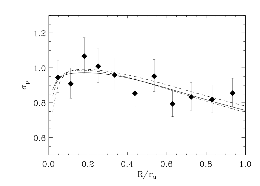
Figure 4: Predicted velocity dispersion profiles from the best-fit mass density models, and the observed $\sigma_{p}$ (binned points with 68% error bars). Solid line: $\xi$-model ($a=0.33\,r_{u}$ and $\xi=1.4$); dash-dotted line: NFW-model ($a=0.18\,r_{u}$ and $\xi=1$); dashed line: $\beta$-model ($r_{c}=0.06\,r_{u}$ and $\beta=0.8$).

Figure 5: Mass profiles determined by the Jeans analysis. Solid line: mass profile obtained from the best-fit $\xi$ density model; dash-dotted line: mass profile obtained from the best-fit NFW density model; dashed line: mass profile obtained from the best-fit $\beta$-model. Dotted lines: 68% c.l. for the mass profiles, derived from integration of the density profiles which provide an acceptable fit (to within the 68% c.l.) to the observed $\sigma_{p}$ (see Figure 3).

The allowed 68% confidence level (c.l. hereafter) isocontours in the space of $(a,\xi)$, and $(r_{c},\beta)$ parameters are shown in Figure 3. The confidence levels are determined as described in Avni (1976), for two interesting parameters. Clearly, density models with a wide range of parameters provide an acceptable fit to our data. In particular, the best fit to the $\xi$-model is obtained for $a=0.33\,r_{u}$ and $\xi=1.4$, with a reduced $\chi^{2}=0.6$. A standard NFW model (corresponding to the case $\xi=1.0$) provides an almost equally good fit to the data. The best fit NFW model is obtained for $a=0.18\,r_{u}$, as expected for halos with $\sigma_{p}\simeq 500$ km s${}^{-1}\;$in a $\Lambda$CDM Universe. Also acceptable are the density models with a core ($\xi=0$), in which case the scale is constrained to be small, $a\simeq 0.1\,r_{u}$. Consistently, the allowed values of $r_{c}$ for the $\beta$-model are also rather small. The best-fit is obtained for $r_{c}=0.06\,r_{u}$ and $\beta=0.8$, which are close to the values found by Girardi et al. (1998) for the number density profiles of cluster galaxies. Core-radii $r_{c}\geq 0.2\,r_{u}$ ($r_{c}\geq 0.3\,r_{u}$) are excluded at the 68% (90%) c.l.. A standard King (1962) profile ($\beta=1.0$) with $r_{c}=0.14\,r_{u}$ is also an acceptable fit; these values are close to those obtained by Adami et al. (1998) for the number density profiles of cluster galaxies.

In Figure 4 we show the predicted velocity dispersion profiles for the best-fit $\xi$- (solid line), $\xi=1$ NFW (dash-dotted line), and $\beta$- (dashed-line) models, as well as the observed (binned) $\sigma_{p}$-profile.

We obtain the 68% c.l. for the cluster mass profile by integrating the mass density profiles which provide 68% c.l. acceptable fits to the observed $\sigma_{p}$-profile. The mass profiles determined via integration of the best-fit mass density profiles, and the 68% c.l. for the cluster mass profile are shown in Figure 5. The mass is in the normalized units of our ensemble cluster, i.e. $r_{u}\sigma_{p}^{2}/G$, which corresponds to $\approx 5\times 10^{13}$ $h^{-1}\ M_{\odot}\;$, for the average value of $\sigma_{p}\simeq 500$ km s${}^{-1}\;$of the 43 clusters that constitute our ensemble cluster. We call $M_{\rm n}$  the normalized mass. The mass profiles obtained from the best-fit $\xi$- and $\beta$- mass density models are very similar in the fitted region ($r\leq r_{u}$). The total mass at $r\leq r_{u}$ appears to be determined with an accuracy of $\simeq\pm 8$%.

3.2 The caustic approach

Figure 6: ’Optimal caustic’ and the distribution of galaxies from the ensemble cluster in the space of normalized clustercentric distances and velocities. Large dots indicate the cluster members used to determine $\overline{v_{\rm n}^{2}}(\leq\overline{R})$ – see text.

In order to extend the determination of the cluster mass profile beyond the virialization radius $r_{u}\simeq r_{200}$, we must rely on methods that do not assume the cluster dynamical equilibrium, since this is unlikely to hold in the external cluster regions. The method we use is that of Diaferio & Geller (1997) and D99. These authors have shown that the velocity field in the cluster outskirts is determined by the cluster mass distribution, via

$$GM(<r)-GM(<r_{0})=\int_{r_{0}}^{r}{\cal A}^{2}(x)\,{\cal F}_{\beta}(x)\,dx,$$ (5)

where ${\cal A}$ is the amplitude of the caustics described by the galaxy distribution in the space of normalized clustercentric distances and velocities, and ${\cal F}_{\beta}$ is a function of the gravitational potential and the anisotropy profile.

We determine the caustics with an adaptive kernel method, as described in D99 (see also Pisani 1996). Following Diaferio & Geller (1997) and Geller et al. (1999), we scale the smoothing-window sizes along the axes of clustercentric distance and velocities before applying the adaptive kernel method, in such a way as to give equal weights to the typical uncertainties of normalized clustercentric distances and velocities. In our sample the median velocity uncertainty is 90 km s^-1, or 0.2 in normalized units. The positional uncertainty of a galaxy is of the order of the galaxy size, i.e. about 20 $h^{-1}$ kpc, or 0.02 in normalized units. We therefore take $q=10$ as the ratio between the smoothing-window sizes on the two axes. Geller et al. (1999) have shown that the mass profile determination is largely independent on the precise choice of $q$. As in Geller et al. (1999), we symmetrize the caustics with respect to the mean cluster velocity.

Figure 7: Function ${\cal F}_{\beta}$ for the determination of the cluster mass profile with the caustic method. The dashed line shows the value ${\cal F}_{\beta}=0.5$ used by Geller et al. (1999).

Following D99 and Geller et al. (1999), we choose the caustic that minimizes the function:

$$S\equiv\mid\overline{v_{esc}^{2}}-4\overline{v_{\rm n}^{2}}(\leq\overline{R})\mid^{2}.$$ (6)

The $\overline{v_{esc}^{2}}$ term is determined from the caustic amplitude, and $\overline{v_{\rm n}^{2}}(\leq\overline{R})$ is the normalized velocity dispersion of the cluster members contained within $\overline{R}$, the average clustercentric distance of all cluster members. As described in § 3.1 our fiducial sample of cluster members does not include late-type spirals and is restricted to galaxies within $r_{u}$. We show in Figure 6 the caustic that minimizes the $S$ function (see eq. 6). Hereafter, we refer to this caustic as the ’optimal caustic’.

In order to translate the optimal caustic amplitude into a mass profile, we must know the function ${\cal F}_{\beta}$. This function actually depends on the gravitational potential one is willing to determine. However, numerical simulations show that this dependence is small at sufficiently large distances from the cluster center (D99). Diaferio & Geller (1997) and Geller et al. (1999) used the simple approximation ${\cal F}_{\beta}\equiv 0.5$, but this is not really supported by the results of D99 (see Figure 3 in D99’s paper). In our analysis we adopt a non-constant ${\cal F}_{\beta}$ (see Figure 7) which is a smooth approximation of the result obtained by D99 for a $\Lambda$CDM cosmology. The resulting mass function is shown in Figure 8 (top panel). The c.l.’s on this mass function are determined as in Geller et al. (1999). For the sake of comparison, we also show the mass function one would obtain by adopting ${\cal F}_{\beta}=0.5$.

As can be seen from the top panel of Figure 8, the mass profiles determined from the same optimal caustic, using different ${\cal F}_{\beta}$ functions, can differ considerably. As a matter of fact, the choice of ${\cal F}_{\beta}$ constitutes the dominant source of uncertainty in this method. Note however that the mass profile determined using a non-constant ${\cal F}_{\beta}$ is in remarkable consistency with the mass profile determined via the Jeans analysis (see § 3.1).

In order to reduce the systematic errors in the mass profile, it is better to avoid using the caustic method in the central cluster regions. In fact, the main advantage of the caustic method lies in its applicability beyond the virialized central region, where classical methods fail, but classical methods may prove superior in the central region, where the caustic method suffers from the uncertainty in the function ${\cal F}_{\beta}$. We can therefore take advantage of the constraints imposed by the Jeans analysis on the mass interior to $r_{u}$, and compute the mass from the caustic method only at $r>r_{u}$ (i.e. we set $r_{0}=r_{u}$ in eq. 5). By doing this we reduce the uncertainty in the mass profile determined via the caustic method, because the radial dependence of ${\cal F}_{\beta}$ is much smaller at large radii than in the central region (see Figure 2 in D99). The combined mass profile from the Jeans and the caustic approach is shown in the bottom panel of Figure 8. Clearly, the mass profiles determined with different choices of ${\cal F}_{\beta}$ are now in good agreement, since we compute them only for $r>r_{u}$. The uncertainty on the total mass at $r=2r_{u}$ is $\approx\pm 15$%.

We note that the mass profile determined by the caustic method follows very closely the extrapolation of the best-fit $\xi$-profile out to $r=2r_{u}$. The best-fit $\beta$-profile is somewhat steeper, but well within the 68% confidence region of the caustic mass profile.

Figure 8: Mass profiles determined by the caustic method. Top panel: the mass profile determined using the ${\cal F}_{\beta}$ function (solid line) within its 68% c.l. (dotted lines). The dashed line shows the mass profile determined using ${\cal F}_{\beta}=0.5$. Thin solid lines truncated at $r=r_{u}$ indicate the 68% c.l.’s on the mass profile determined by the Jeans analysis (see § 3.1). Bottom panel: the combined mass profile determined via the Jeans and the caustic methods. The two profiles at $r\leq r_{u}$ are obtained by integration of the best-fit $\xi$- and $\beta$- density models (solid and dashed lines, respectively). The two profiles at $r>r_{u}$ are obtained via the caustic method, by imposing continuity with the $\xi$ mass profile at $r=r_{u}$, assuming either a variable or a constant ${\cal F}_{\beta}$ (dash-dotted and long-dashed lines, respectively). Dotted lines indicate the 68% c.l.’s on the mass profile determined via the Jeans analysis at $r\leq r_{u}$, and via the caustic analysis at $r>r_{u}$ (continuity is imposed at $r=r_{u}$).

4 THE MASS-TO-NUMBER DENSITY PROFILE

In § 3.2 we have determined the average cluster mass profile out to $r=2r_{u}$. We obtain the average cluster mass density profile, $\rho$, by numerical differentiation of the mass profile shown in the bottom panel of Figure 8 (indicated by the solid line up to $r=r_{u}$, and by the dash-dotted line at larger radii). We determine the 68% confidence interval on this density profile by constructing a set of density profiles which are built non-parametrically from the differentiation of several mass profiles spanning the allowed 68% confidence region. In building these density profiles we impose the physical condition of a negative logarithmic derivative of the mass density at all radii.

In order to determine the 3-dimensional number density profile, $\nu$ (and its confidence intervals), up $r=2r_{u}$, we use MAPELN. In this case we do not exclude late-type spiral members, since we are interested in the total number of galaxies in the cluster, irrespective of their kinematics. Since the 2dFGRS is complete in apparent magnitude, and our 43 clusters span a significant redshift range (0.02–0.13), we need to impose an absolute magnitude limit to ensure the same sampling of the luminosity functions of all our 43 clusters. We therefore select the 399 cluster members brighter than the k-corrected (Madgwick et al., 2002) absolute magnitude $M_{b_{J}}=-19.3+5\log h$, which is the magnitude of the faintest member of the most distant among our 43 clusters, APM 294 (see § 2). This magnitude is sufficiently bright as to avoid possible problems related to the increase in the number of dwarf galaxies with clustercentric distance (see, e.g. Beijersbergen et al., 2002; Durret et al., 2002; Lobo et al., 1997).

Since the cluster membership assignment is problematic beyond $r_{u}$, we correct the MAPELN density profile at larger distances, by making use of the optimal caustic. Specifically, beyond $r_{u}$ we multiply the MAPELN density profile by the fraction of cluster members which are contained within the optimal caustic in each given radial bin. This fraction is 0.8 on average, i.e. $\sim 20$% of our (presumed) cluster members beyond $r_{u}$ could be interlopers.

Figure 9: Mass-to-number density profiles for the ensemble cluster (solid lines) and best-fit constants (dashed lines). Top panel: the number density profile is determined for the sample of all cluster members brighter than $M_{b_{J}}=-19.3+5\log h$. Bottom panel: the number density profile is determined for the sample of early-type cluster members brighter than $M_{b_{J}}=-19.3+5\log h$. The error bars account for the uncertainties in both the mass and the number density profiles. The vertical scale is in normalized units (see § 3.1).

The mass-to-number density ratio as a function of the clustercentric radial distance is shown in Figure 9 (upper panel). The vertical scale in this plot is in normalized units (see § 3.1). The irregular behavior at radii larger than $r_{u}$ is due to the use of a non-parametric mass profile estimator (the caustic method). The bump at $r\simeq r_{u}$ is related to the fact that we have joined the mass profile determined from the Jeans analysis and the mass profile determined from the caustic method, without imposing a continuous derivative. Apart from obvious irregularities, one can notice an almost monotonous decrease from $r\simeq 0.3\,r_{u}$ to the outermost radius. We test the null hypothesis of a constant mass-to-number density profile by the $\chi^{2}$ method. The null hypothesis is fully consistent with the data (3.7% c.l.) when only the inner $r\leq r_{u}$ region is considered, but it is rejected (99.9% c.l.) over the full radial range ($0<r<2r_{u}$). Had we not corrected for the presence of doubtful cluster members at radii larger than $r_{u}$, the decrease would have been (marginally) even stronger.

In Figure 9 (lower panel) we also plot the mass-to-number density ratio for the sample of 299 early-type, i.e. $\eta\leq-1$ (Madgwick et al., 2002), cluster members brighter than $M_{b_{J}}=-19.3+5\log h$. The mass-to-number density profile is somewhat flatter, as expected, since the early-type cluster galaxies have the steepest number density profile among cluster galaxy populations (e.g. Dressler, 1980; Biviano et al., 2002). In this case, the mass-to-number density profile is consistent with being constant, not only within the central $r<r_{u}$ region (0.2% c.l.), but also up to $2r_{u}$ (74.2% c.l.).

5 DISCUSSION

In our analysis we have determined the mass and mass-to-number density profiles of galaxy clusters out to $\sim 2r_{200}$. We find that both cuspy profiles and profiles with a core are acceptable. Best-fits to the inner $\raise-2.0pt\hbox{\hbox to0.0pt{\hbox{$\sim$}\hss}\raise 5.0pt\hbox{$<$}\ }r_{200}$ region are found for a $\beta$-profile (see eq. 4) with $\beta=0.8$ and $r_{c}\simeq 0.06\,r_{200}$, or a $\xi$-profile (see eq. 3) with $\xi=1.4$ and $a\simeq 0.33\,r_{200}$. Acceptable fits are also found for a King (1962) profile with $r_{c}\simeq 0.14\,r_{200}$ and a NFW profile with $a\simeq 0.18\,r_{200}$. Density profiles with very large core-radii ($r_{c}\raise-2.0pt\hbox{\hbox to0.0pt{\hbox{$\sim$}\hss}\raise 5.0pt\hbox{$>$}\ }0.3\,r_{200}$) are ruled out (90% c.l.). The density profiles that provide the best-fits to the data in the inner $\raise-2.0pt\hbox{\hbox to0.0pt{\hbox{$\sim$}\hss}\raise 5.0pt\hbox{$<$}\ }r_{200}$ region, also provide a reasonable description of the cluster gravitational potential at larger radii, out to $\sim 2r_{200}$.

Let us compare our results with previous mass-profile determinations. From the analysis of the CNOC cluster survey data-set Carlberg et al. (1997a) and vdM00 conclude that the average mass profile of galaxy clusters is well described by the NFW’s analytic form, with a scale $a\simeq 0.25\,r_{200}$, although other profiles are equally acceptable. Their best-fit NFW scale is slightly larger than ours, but not significantly so. Note anyway that the CNOC clusters are on average more massive than the 43 clusters in our sample, so they are expected to be less concentrated and have a larger NFW scale.

Geller et al. (1999) find that the NFW profile provides a good fit to the Coma mass profile, while a softened isothermal sphere does not. Similarly, Rines et al. (2000) are able to rule out a singular isothermal sphere for the mass profile of the cluster A576, while a NFW profile is a good fit to the observed mass profile. Both the results of Geller et al. (1999) and those of Rines et al. (2000) are based on the caustic analysis.

Similar conclusions about the cluster mass profile are reached by Markevitch et al. (1999) using X-ray data. Both the cluster A2199 and the cluster A496 have mass profiles remarkably well approximated by NFW models, and deviate from the isothermal mass profile (which is too steep). On the other hand, Ettori, De Grandi & Molendi (2002) find that about half of 22 nearby clusters of galaxies have an X-ray determined mass density profile which is better fitted by a King (1962)’s rather than a NFW model. In their X-ray analyses of 12 galaxy clusters, Durret et al. (1994) find that the King profile provides a good fit to the mass density distribution, but with very small core-radii ($\simeq 15$ $h^{-1}$ kpc).

Useful constraints are derived from the gravitational lensing analysis. Most authors (Clowe, 2000; Clowe & Schneider, 2001; Lombardi et al., 2000; Bautz, Arabadjis, & Garmire, 2002) conclude in favor of a NFW mass profile and against an isothermal sphere mass distribution, except perhaps Sheldon et al. (2001).

Our results are in agreement with the claims in support of a NFW mass density profile and against both a softened and a singular isothermal sphere mass profiles, which both increase faster with radius than our observed cluster mass profile. We stress however that our data do not rule out the presence of a core in galaxy clusters, although this core has to be very small, of the order of the size of a galaxy. Interestingly, our formal best-fit for a NFW profile is obtained for $a\simeq 0.18\,r_{200}$, which is mid-way between the formal best-fit obtained for the CNOC clusters by vdM00 and the formal best-fit obtained for the poor galaxy systems by Mahdavi et al. (1999). Since our clusters are of intermediate mass between the CNOC clusters and the poor systems of galaxies of Mahdavi et al. (1999), a scaling of $a$ with the mass of the system is suggested, as expected from numerical simulations (NFW).

Our most intriguing result is the significant decrease of the mass-to-number density ratio at radii greater than $\sim 0.3r_{200}$. The mass per galaxy at $r_{200}<r<2r_{200}$ is only about half the mass per galaxy in the cluster central regions. Although we do not derive the mass-to-light profile (which would require an analysis of the cluster luminosity function and it is beyond the scope of this paper), this is unlikely to be constant. In fact, for the mass-to-light profile to be flat, a strong luminosity segregation over the entire radial range out to $\sim 2r_{200}$ is required. Apart from the segregation of the very bright galaxies, which only concerns the cluster cores (e.g. Biviano et al., 2002), luminosity segregation in clusters is also observed as a change of the number ratio of dwarf to giant galaxies with radius(e.g. Beijersbergen et al., 2002; Durret et al., 2002; Lobo et al., 1997). However, the luminosity segregation of dwarf galaxies is not relevant in our case, since our number density profile is determined only on galaxies brighter than $M_{b_{J}}=-19.3+5\log h$, which is only $\sim 0.3$ magnitudes fainter than $M^{\star}$ in the Schechter luminosity function for early-type galaxies (Madgwick et al., 2002). We do not find evidence of luminosity segregation in our sample of members brighter than $M_{b_{J}}=-19.3+5\log h$, as their absolute magnitudes and clustercentric distances are uncorrelated (52% c.l., according to a Spearman rank correlation test).

Our mass-to-number density profile implies a mass distribution more concentrated than the galaxies. Since the hot X-ray emitting gas is less concentrated than the galaxies (e.g. Eyles et al., 1991; Durret et al., 1994; Cirimele et al., 1997), our result also implies that the dark matter distribution is more concentrated than the baryonic matter distribution.

Previous determinations of the mass-to-light (or mass-to-number) profiles have provided evidences both in favor (Carlberg et al., 1997a; Cirimele et al., 1997; Mahdavi et al., 1999; van der Marel et al., 2000; Rines et al., 2001) and against (Koranyi et al., 1998; Rines et al., 2000; Carlberg et al., 2001) a constant mass-to-light profile. Koranyi et al. (1998) find an increasing mass-to-light profile in the poor cluster AWM7, from the center to $\sim 0.2$ $h^{-1}$ Mpc. Such an increase is also seen in our data (see Figure 9) but it is not significant. Rines et al. (2000) find that the mass-to-light profile decreases with clustercentric radius, in consistency with our finding. Carlberg et al. (2001) find an increasing mass-to-light profile in galaxy groups. Clearly, a general consensus on the relative distribution of dark and baryonic matter in galaxy systems is still lacking. Part of the discrepancy among different authors can arise from the use of different photometric bands (Rines et al., 2001). Cluster members are redder in the cluster center, so that blue-band selected cluster samples (like ours) should be characterized by flatter number density profiles, and hence steeper mass-to-number density profiles, as compared to samples selected in the near-infrared. Our mass-to-number density profile indeed becomes flatter, and consistent with being constant, when only early-type (and hence redder) cluster members are considered (see Fig. 9).

Does our result invalidates the use of simple mass estimators based on the light traces mass hypothesis? Probably not. In fact, our mass-to-number density profile does not significantly deviate from a constant when we restrict the analysis to the virialized region ($r\leq r_{200}$), or when only the early-type galaxies are considered.

6 SUMMARY

We use the June 2001 public release of the 2dFGRS to construct a sample of 4947 galaxies with redshifts in the region of 43 clusters, reaching out to $\sim 2r_{200}$. 1345 cluster members are selected with the method of Fadda et al. (1996). We build an ensemble cluster profile from this sample, using $r_{200}$ and $\sigma_{p}$ of each cluster to normalize the clustercentric radii and velocities of all galaxies.

We determine the mass profile of this ensemble cluster by two independent methods, namely those of vdM00 and D99. The method of vdM00 is based on the solution of the Jeans equation, and can only be applied in conditions of dynamical equilibrium. We therefore apply it on the subsample of cluster members within the virial radius, $r_{200}$. We exclude late-type spirals from this sample since these galaxies have been shown in the literature to be characterized by anisotropic orbits (e.g. Mohr, 1996; Biviano et al., 1997). The method of D99 can usefully be applied to the whole sample of galaxies in the cluster region, since it does not require dynamical equilibrium. We use it to constrain the cluster mass profile beyond the virial radius, and out to the limit we imposed on our sample, $\sim 2r_{200}$.

We find very good agreement between the mass profiles determined using the two methods. The mass profile from the center to $\sim 2r_{200}$ is remarkably well fitted by a $\xi$-model (eq. 3) with $a\simeq 0.33\,r_{200}$ and $\xi=1.4$, but many other models provide acceptable fits, including NFW models and models with a small core ($r_{c}\raise-2.0pt\hbox{\hbox to0.0pt{\hbox{$\sim$}\hss}\raise 5.0pt\hbox{$<$}\ }0.2r_{200}$). We find an uncertainty on the total mass of $\approx\pm 8$% at the virial radius, and $\approx\pm 15$% at two virial radii.

We determine the mass-to-number density profile of the ensemble cluster. It is fully consistent with a constant from the center to $\sim r_{200}$, but it significantly decreases at larger radii. The decreasing trend is however not significant when the number density profile is computed on the early-type galaxies only.

Table 1: The sample of 43 clusters

Name	RAJ2000	DECJ2000	Nm	Nm	$\overline{v}$	$\sigma_{p}$
	(h m s)	(∘ ′ ′′)		$(R\leq r_{u})$	(km s-1)	(km s-1)
ACO 419	03 06 15.3	-23 55 57	41	30	20499	681
ACO 892	09 51 03.1	00 49 43	18	13	28130	435
ACO 957	10 11 13.7	-00 40 32	68	43	13648	653
ACO 978	10 17 58.5	-06 15 41	31	22	16371	534
ACO 993	10 19 34.5	-04 38 46	62	33	16368	503
ACO 1098	10 45 26.8	-03 40 39	25	14	20699	465
ACO 1308	11 30 30.2	-03 43 53	20	10	15496	287
ACO 1364	11 40 56.5	-01 27 40	37	24	31681	542
ACO 1373	11 42 55.9	-02 10 23	28	20	38892	568
ACO 1750	13 28 45.0	-01 28 46	37	24	25187	649
ACO 2660	23 43 08.8	-26 06 42	38	12	15968	825
ACO 2726	00 04 49.4	-28 21 52	31	15	18220	339
ACO 2734	00 08 47.2	-29 05 04	67	43	18437	625
ACO 2915	01 26 25.6	-29 17 17	25	16	25877	546
ACO 2967	02 00 30.9	-28 30 50	14	11	33036	498
ACO 2981	02 07 38.0	-27 37 23	14	10	32484	382
ACO 3042	02 41 05.0	-27 06 59	17	12	31161	404
ACO 3814	21 46 25.2	-30 58 31	30	24	35819	836
ACO 3837	22 06 21.5	-27 33 60	25	16	27390	366
ACO 4044	23 46 53.2	-27 15 59	22	15	32917	417
ACO 4049	23 50 03.8	-28 56 56	14	5	17743	418
ACO 4053	23 52 10.7	-27 57 05	45	34	21451	488
ACO S246	02 17 39.8	-27 26 57	15	6	17776	181
ACO S301	02 47 28.9	-31 21 39	100	52	6772	464
ACO S340	03 18 04.4	-27 12 06	22	14	20840	328
ACO S983	21 57 12.4	-19 23 20	9	5	17246	130
ACO S1127	23 25 38.4	-29 24 33	38	20	31259	767
APM 171	01 22 38.9	-29 45 42	22	7	29038	449
APM 294	02 45 06.8	-27 45 38	26	13	39891	562
APM 311	02 52 12.3	-33 40 18	27	20	32608	467
APM 416	03 32 28.6	-29 07 35	38	14	31360	656
APM 715	21 45 56.5	-27 53 34	21	12	21726	625
APM 880	23 15 54.9	-27 25 06	27	9	25126	351
EDCC 69	21 56 06.8	-28 42 06	24	16	6385	275
EDCC 129	22 16 11.4	-24 36 22	19	12	11400	397
EDCC 148	22 25 39.8	-24 41 59	36	16	23395	539
EDCC 153	22 29 38.2	-31 26 48	23	16	17130	520
EDCC 155	22 29 20.3	-25 39 05	44	23	10118	520
EDCC 445	00 25 58.7	-27 46 02	48	16	18511	483
EDCC 601	01 51 25.0	-33 23 52	23	16	29200	468
EDCC 623	02 04 22.6	-28 37 55	21	13	25369	717
EDCC 641	02 13 53.6	-27 47 19	25	15	31236	340
EDCC 642	02 14 16.4	-29 13 29	28	12	32513	375

References

- Abell, Corwin, & Olowin (1989) Abell, G. O., Corwin, H. G. Jr., & Olowin, R. P. 1989, ApJS, 70, 1
- Adami et al. (1998) Adami, C., Biviano, A., & Mazure, A. 1998, A&A, 331, 439
- Alonso et al. (1999) Alonso, M. V., Valotto, C., Lambas, D.G., & Muriel, H. 1999, MNRAS, 308, 618
- Avni (1976) Avni, Y. 1976, ApJ, 210, 642
- Barrena et al. (2002) Barrena, R., Biviano, A., Ramella, M., Falco, E.E., Seitz, S. 2002, A&A, 386, 816
- Bautz, Arabadjis, & Garmire (2002) Bautz, M. W., Arabadjis, J. S, & Garmire, G. P. 2002, preprint (astro-ph/0202338)
- Beers et al. (1990) Beers, T. C., Flynn, K., & Gebhardt, K. 1990, AJ, 100, 32
- Beijersbergen et al. (2002) Beijersbergen, M., Hoekstra, H., van Dokkum, P. G., & van der Hulst, T. 2002, MNRAS, 329, 385
- Binney & Tremaine (1987) Binney, J. & Tremaine, S. 1987, Galactic Dynamics (Princeton: Princeton University Press)
- Biviano (2002) Biviano, A. 2002, in Tracing Cosmic Evolution with Galaxy Clusters, ed. S. Borgani, M. Mezzetti, & R. Valdarnini (San Francisco: ASP) in press
- Biviano et al. (1992) Biviano, A., Girardi, M., Giuricin, G., Mardirossian, F., & Mezzetti, M. 1992, ApJ, 396, 35
- Biviano et al. (1997) Biviano, A., Katgert, P., Mazure, A., Moles, M., den Hartog, R., Perea, J., & Focardi, P. 1997, A&A, 321, 84
- Biviano et al. (2002) Biviano, A., Katgert, P., Thomas, T., & Adami, C. 2002, A&A, 387, 8
- Carlberg et al. (1997b) Carlberg, R. G., et al. 1997b, ApJ, 476, L7
- Carlberg et al. (1997a) Carlberg, R. G., et al. 1997a, ApJ, 485, L13
- Carlberg et al. (2001) Carlberg, R. G., Yee, H. K. C., Morris, S. L., Lin, H., Hall, P. B., Patton, D. R., Sawicki, M., & Shepherd, C. W. 2001 ApJ, 552, 427
- Cavaliere & Fusco-Femiano (1978) Cavaliere, A., & Fusco-Femiano, R. 1978 A&A, 70, 677
- Cirimele et al. (1997) Cirimele, G., Nesci, R., & Trevese, D. 1997, ApJ, 475, 11
- Clowe (2000) Clowe, D., Luppino, G. A., Kaiser, N., & Gioia, I. M. 2000, ApJ, 539, 540
- Clowe & Schneider (2001) Clowe, D., & Schneider, P. 2001, A&A, 379, 384
- Colless et al. (2001) Colless, M., et al. 2001, MNRAS, 328, 1039
- Dalton et al. (1997) Dalton, G. B., Maddox, S. J., Sutherland, W. J., & Efstathiou, G. 1997, MNRAS, 289, 263
- Danese et al. (1980) Danese, L., De Zotti, C., & di Tullio, G. 1980, A&A, 82, 322
- De Propris et al. (2002) De Propris, R., et al. 2002, MNRAS, 329, 87 (DP02)
- Diaferio (1999) Diaferio, A. 1999, MNRAS, 309, 610 (D99)
- Diaferio & Geller (1997) Diaferio, A., & Geller, M. J. 1997, ApJ, 481, 633
- Dressler (1980) Dressler, A. 1980, ApJ, 236, 351
- Durret et al. (2002) Durret, F., Adami, C., & Lobo, C. 2002, A&A, in press, astro-ph/0207195
- Durret et al. (1994) Durret, F., Gerbal, D., Lachièze-Rey, M., Lima-Neto, G., & Sadat, R. 1994, A&A, 287, 733
- Ellingson et al. (1998) Ellingson, E., Yee, H. K. C., Abraham, R. G, Morris, S. L., & Carlberg, R. G. 1998, ApJS, 116, 247
- Ettori et al. (2002) Ettori, S., De Grandi, S., & Molendi, S. 2002, A&A, in press (astro-ph/0206120)
- Eyles et al. (1991) Eyles, C. J., Watt, M. P., Bertram, D., Church, M. J., Ponman, T. J., Skinner, G. K., & Willmore, A. P. 1991, ApJ, 376, 23
- Fadda et al. (1996) Fadda, D., Girardi, M., Giuricin, G., Mardirossian, F., & Mezzetti, M. 1996, ApJ, 473, 670
- Fasano & Franceschini (1987) Fasano, G., & Franceschini, A. 1987, MNRAS, 225, 155
- Fusco-Femiano & Menci (1998) Fusco-Femiano, R., & Menci, N. 1998, ApJ, 498, 95
- Geller et al. (1999) Geller, M. J., Diaferio, A., & Kurtz, M. J. 1999, ApJ, 517, L23
- Girardi et al. (1996) Girardi, M., Fadda, D., Giuricin, G., Mardirossian, F., Mezzetti, M., & Biviano, A. 1996, ApJ, 457, 61
- Girardi et al. (1998) Girardi, M., Giuricin, G., Mardirossian, F., Mezzetti, M., & Boschin, W. 1998, ApJ, 505, 74
- Gonzales-Casado et al. (1994) Gonzalez-Casado, G., Mamon, G., Salvador-Solé, E. 1994, ApJ, 433, L61
- Hernquist (1990) Hernquist, L. 1990, ApJ, 356, 359
- Katgert et al. (1996) Katgert, P., et al. 1996, A&A, 310, 8
- Katgert et al. (1998) Katgert, P., Mazure, A., den Hartog, R., Adami, C., Biviano, A., & Perea, J. 1998, A&AS, 129, 399
- King (1962) King, I. R. 1962, AJ, 67, 471
- Koranyi et al. (1998) Koranyi, D. M., Geller, M. J., Mohr, J. J., & Wegner, G. 1998, AJ, 116, 2108
- Lobo et al. (1997) Lobo, C., Biviano, A., Durret, F., Gerbal, D., Le Fèvre, O., Mazure, A., & Slezak, E. 1997, A&A, 317, 385
- Lombardi et al. (2000) Lombardi, M., Rosati, P., Nonino, M., Girardi, M., Borgani, S., & Squires, G. 2000, A&A, 363, 401
- Lumsden et al. (1992) Lumsden, S. L., Nichol, R. C., Collins, C. A., & Guzzo, L. 1992, MNRAS, 258, 1
- Madgwick et al. (2002) Madgwick D. S., et al. 2002, MNRAS, 333, 133
- Mahdavi et al. (1999) Mahdavi, A., Geller, M. J., Böhringer H., Kurtz, M. J., & Ramella, M., 1999, ApJ, 518, 69
- Mamon (1995) Mamon, G. 1995, in 3rd Chalonge Colloque Cosmologie, ed. H. de Vega & N. S. Sánchez (Singapore: World Scientific), 95 (astro-ph/9511101)
- Mamon (2000) Mamon, G. 2000, in ASP Conf. Ser. 197, Galaxy Dynamics: from the Early Universe to the Present, ed. F. Combes, G.A. Mamon, & V. Charmandaris (San Francisco: ASP), 367
- Markevitch et al. (1999) Markevitch, M., Vikhlinin, A., Forman, W. R., & Sarazin, C. L. 1999, ApJ, 527, 545
- Mazure et al. (1996) Mazure, A., et al. 1996, A&A, 310, 31
- Merritt (1987) Merritt, D. 1987, ApJ, 313, 121
- Merritt & Gebhardt (1994) Merritt, D., & Gebhardt, K. 1994, in Clusters of Galaxies, ed. F. Durret, A. Mazure, & J. Tran Than Van, (Gif-sur-Yvette: Editions Frontières), 11
- Merritt & Tremblay (1994) Merritt, D., & Tremblay, B. 1994, AJ, 108, 514
- Mohr (1996) Mohr, J. J., Geller, M. J., Fabricant, D. G., Wegner, G., Thorstensen, J., & Richstone, D. O. 1996, ApJ, 470, 724
- Navarro, Frenk & White (1997) Navarro, J. F., Frenk, C. S., & White, S. D. M. 1997, ApJ, 490, 493 (NFW)
- Norberg et al. (2001) Norberg, P. et al. 2002, MNRAS, 328, 64
- Pisani (1993) Pisani, A. 1993, MNRAS, 265, 706
- Pisani (1996) Pisani, A. 1996, MNRAS, 278, 697
- Reisenegger et al. (2000) Reisenegger, A., Quintana, H., Carrasco, E. R., & Maze, J. 2000, AJ, 120, 523
- Rines et al. (2000) Rines, K., Geller, M. J., Diaferio, A., Mohr, J. J., & Wegner, G. A. 2000, AJ, 120, 2338
- Rines et al. (2001) Rines, K., Geller, M. J., Kurtz, M. J., Diaferio, A., Jarrett, T. H., & Huchra, J. P. 2001, ApJ, 561, L41
- Sheldon et al. (2001) Sheldon, E. S., et al. 2001, ApJ, 554, 881
- Smith (1936) Smith, S. 1936, ApJ, 83, 23
- The & White (1986) The, L. S., & White, S. D. M. 1986, AJ, 92, 1248
- van der Marel (1994) van der Marel, R. P. 1994, MNRAS, 270, 271
- van der Marel et al. (2000) van der Marel, R. P., Magorrian, J., Carlberg, R. G., Yee, H. K. C., & Ellingson, E. 2000, AJ, 119, 2038 (vdM00)
- Wegner et al. (2001) Wegner, G., et al., 2001, AJ, 122, 2893
- Yee et al. (1996) Yee, H. K. C., Ellingson, E., & Carlberg, R. G. 1996, ApJS, 102, 269
- Zwicky (1933) Zwicky, F. 1933, Helv. Phys. Acta, 6, 10
- Zwicky (1937) Zwicky, F. 1937, ApJ, 86, 217