The brightness temperature problem in extreme IDV quasars: a model for PKS 0405-385

Abstract

I re-examine the brightness temperature problem in PKS 0405-385 which is an extreme intra-day variable radio quasar with an inferred brightness temperature of $\sim 5\times 10^{14}$ K at 5 GHz, well above the Compton catastrophe limit of $\sim 10^{11}$ K reached when the synchrotron photon energy density exceeds the energy density of the magnetic field. If one takes into account the uncertainty in the distance to the ionized clouds responsible for interstellar scintillation causing rapid intra-day variability in PKS 0405-385 it is possible that the brightness temperature could be as low as $\sim 10^{13}$ K at 5 GHz, or even lower. The radio spectrum can be fitted by optically thin emission from mono-energetic electrons, or an electron spectrum with a low-energy cut-off such that the critical frequency of the lowest energy electrons is above the radio frequencies of interest. If one observes optically thin emission along a long narrow emission region, the average energy density in the emission region can be many orders of magnitude lower than calculated from the observed intensity if one assumed a spherical emission region. I discuss the physical conditions in the emission region and find that the Compton catastrophe can then be avoided using a reasonable Doppler factor. I also show that MeV to 100 GeV gamma-ray emission at observable flux levels should be expected from extreme intra-day variable sources such as PKS 0405-385.

1 Introduction

Rapid variability in intra-day variable (IDV) sources is a long-standing problem as it implies apparent brightness temperatures in the radio regime which may exceed 10¹⁷ K, or requires relativistic beaming with extremely high Doppler factors, coherent radiation mechanisms, or special geometric effects (Wagner & Witzel 1995). Such high brightness temperatures would be well above the “Compton catastrophe” limit $T_{B}<10^{11}$ K imposed by inverse-Compton scattering (Kellermann & Paulini-Toth 1969, Slysh 1992, Kardashev 2000) when the photon energy density in the emission region exceeds the energy density in the magnetic field. See Krichbaum et al. (2002) and Kedziora-Chudczer et al. (2001) for recent reviews of IDV sources.

The radio-loud quasar PKS 0405-385 is an extreme example of an intra-day variable source with variations on timescales of $t_{\rm IDV}\sim 0.1$ d (Kedziora-Chudczer et al. 1997). Making the assumption that the emission region subtends solid angle $\sim\pi(0.5ct_{IDV}D)^{2}/d_{\theta}^{2}$, where $D$ is the Doppler factor and $d_{\theta}$ is the diameter distance to the source, one can convert the observed 4.8 GHz flux to intensity, and obtain a variability brightness temperature of $T_{\rm var}\approx 10^{21}D^{-2}$ K. In this source, however, Kedziora-Chudczer et al. (1997) interpret the very short variability time as due interstellar scintillation requiring the angular diameter of the most compact component to be $\sim 6$ micro-arcsec, or smaller, corresponding to a solid angle subtended by the IDV core $\Omega=\Omega_{1}$ where $\Omega_{1}\approx 6.79\times 10^{-22}$ sr. The fraction of the total flux they estimated to be associated with this compact IDV core is $S_{c}\approx 0.15$, and the corresponding brightness temperature at 4.8 GHz is $T_{B}\approx 5\times 10^{14}(\Omega_{1}/\Omega)$ K. Although much lower than $T_{\rm var}$, to reconcile this brightness temperature with the $\sim 10^{11}$ K limit would appear to require a very large Doppler factor, $D\sim 10^{3}$, or an even larger angular diameter. To obtain a Doppler factor as large as $10^{3}$ would require not only a jet Lorentz factor of $\Gamma>D/2=500$, but also very close alignment of the jet axis to our line of sight (within $\sim 1/\Gamma<0.1^{\circ}$). The probability of such an alignment occurring by chance is then $\sim 1/4\Gamma^{2}<10^{-6}$, in this case, which makes the very high Doppler factor possibility unattractive.

The effective distance to the interstellar scintillation screen is crucial in determining the angular size of the source, and hence its brightness temperature. The distance used by Kedziora-Chudczer et al. (1997) and Walker (1998) is effectively the scale-height above the Galactic plane of electron number density squared, i.e. $z_{2}=\int_{0}^{\infty}zn_{e}^{2}(z)dz/\int_{0}^{\infty}n_{e}^{2}(z)dz$, for which $z_{2}\approx 500$ pc in the model of Taylor and Cordes (1993) for the free electron distribution in the Galaxy. However, that model was developed mainly for the consistent determination of pulsar distances from dispersion measures, and is most accurate at low galactic latitudes where the majority of pulsars are observed. Taylor and Cordes (1993) themselves warn that one should be aware of uncertainties in their model associated with this. The column density, $\int_{0}^{\infty}n_{e}dz$, is fairly accurately determined, but the scale height of electron number density, $z_{1}=\int_{0}^{\infty}zn_{e}(z)dz/\int_{0}^{\infty}n_{e}(z)dz$, is less well determined, and $z_{2}$ is even less accurately known. For example, in the recent model of Gomez et al. (2001) for the free electron distribution in the Galaxy $z_{2}\sim 300$ pc. It is interesting to note that Beckert et al. (2001) suggest typical distances to the scattering medium of 200 pc, and that a scale height of about 100 pc seems to be required to explain IDV in the case of 0917+624.

Krichbaum et al. (2002) mention the possibility of an extremely clumpy ISM. If this is the case, one could well question the use of an effective screen distance as it could be that the scintillation is due to an individual ionized cloud much nearer to us than the average distance. In fact, if the distribution is highly peaked in the Galactic plane the most probable, rather than average, distance is small. The distance to the ionized cloud responsible for the extreme scattering event in 0954+658 is estimated to be $\sim 150$ pc (Cimo 2002), while Dennett-Thorpe & de Bruyn (2000, 2002) suggest that the scattering region for IDV in J1819+3845 may be located at about 20 pc, and possibly associated with the local bubble. Hence, I believe there could be considerable uncertainty in the distance to the scintillating material responsible for the extreme IDV in PKS 0405-385. If, for example, the distance were smaller by a factor of 5, this would translate into a factor of 25 reduction in the brightness temperature. A brightness temperature of $\sim 2\times 10^{13}$ K at $\sim 5$ GHz for the IDV core in PKS 0405-385 is still high, but I will show that it can be achieved by standard electron synchrotron radiation using quite moderate Doppler factors if one takes into account possible geometries of the emission region.

In a recent paper (Protheroe 2002) I have explored the effect of emission region geometry on flux variability, and on the relationship between observed intensity and energy density for various source geometries for the case of optically thin emission and found that the average energy density in the source can be much less than one would estimate simply from the observed intensity. Although the radio emission from IDV sources is usually assumed to be optically thick, if this is not the case then the above result may also have important implications for IDV sources as the photon energy density responsible for causing the brightness temperature limit may actually be a few orders of magnitude lower than estimated from the intensity. In that case, lower Doppler factors would be required to avoid the Compton catastrophe. In this paper I shall explore the parameter space, including emission region geometry, of models able to reproduce the observed radio emission of the IDV core of PKS 0405-385, and I shall model its spectral energy distribution (SED) from radio to gamma-ray frequencies.

2 Fitting the spectrum of PKS 0405-385

In Fig. 1, I plot the available flux measurements of PKS 0405-385, divided by frequency squared, as gray symbols and gray vertical lines. Contemporaneous VLA and ATCA data (squares and triangles in the 1.4 GHz–43 GHz range) are also re-plotted as black symbols at the observed fluxes multiplied by $S_{c}$, the fraction of the total flux assumed by Kedziora-Chudczer et al. (1997) to be associated with the IDV core. The right axis shows the brightness temperature of the IDV core inferred by Kedziora-Chudczer et al. (1997) assuming the IDV core subtends solid angle $\Omega_{1}$. It is only the IDV core component of these data that I am concerned with fitting. Nevertheless, it is interesting for comparison to include non-contemporaneous data at other wavelengths whose origin may or may not be associated with the same emission region.

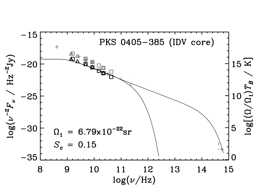
Figure 1: Observed fluxes of PKS 0405-385 divided by $\nu^{2}$ are plotted as gray symbols and vertical lines. Contemporaneous VLA and ATCA data, multiplied by $S_{c}$, are also re-plotted as black symbols and represent the flux from the IDV core. The right-hand axis shows the brightness temperature assuming the IDV core subtends solid angle $\Omega_{1}$. Data: pluses – non-contemporaneous data obtained from the NED archive; triangles and squares – 1996 and 1998 VLA/ATCA data (D. Jauncey personal communication 1999); vertical solid lines – 1993-4 SEST data (Tornikoski et al. 1996); dashed vertical lines at 230 GHz and $4.3\times 10^{14}$ Hz – (S. Wagner personal communication 1999). The solid curves are fits for synchrotron radiation by mono-energetic electrons with $\nu_{1}=10^{9.1}$ Hz and $\nu_{c}=10^{11}$ Hz (left) or $\nu_{c}=10^{13.65}$ Hz (right).

Over the 1.4 GHz–43 GHz range, the intensity can be fitted well by $I_{\nu}\propto\nu^{1/3}$ ($T_{B}\propto\nu^{-5/3}$). Such a spectrum would occur naturally if the emission were optically thin and if this frequency range were well below the critical frequency of the lowest energy electron. Note that for an XSelectron with Lorentz factor $\gamma$ the critical frequency is

$$\nu_{c}={3\gamma^{2}eB_{\perp}\over 4\pi m_{e}c}=4.19\times 10^{6}\gamma^{2}B_{\perp}\mbox{ Hz}$$ (1)

where $e$ is the electron charge (statcoulombs), $B_{\perp}$ is the component of magnetic field (gauss) perpendicular to the electron velocity, and $m_{e}$ is the electron mass (grams). Such an electron spectrum could occur naturally if the electrons were produced as secondaries of other particles, e.g. Bethe-Heitler pair-production by relativistic protons, or if explosive re-connection were responsible for electron acceleration. For the purposes of this paper, I shall adopt a mono-energetic electron distribution.

For a mono-energetic isotropic electron distribution the synchrotron emission coefficient is given by

$$j_{\nu}={P(\nu)\over 4\pi}={\sqrt{3}e^{3}B_{\perp}n_{e}\over 4\pi m_{e}c^{2}}F(x)$$ (2)

where $n_{e}$ is the electron number density (cm^-3), $x=\nu/\nu_{c}$ and $F(x)\equiv x\int_{x}^{\infty}K_{5/3}(\xi)d\xi$ (see e.g. Rybicki and Lightman 1979). At low frequencies $\nu\ll\nu_{c}$

$$F(x)={4\pi\over\sqrt{3}\Gamma\!\left({1\over 3}\right)}\left({x\over 2}\right)^{1/3},\;\;\;\;j_{\nu}={e^{3}B_{\perp}n_{e}\over\Gamma\!\left({1\over 3}\right)m_{e}c^{2}}\left({x\over 2}\right)^{1/3}.$$ (3)

The absorption coefficient for an isotropic electron distribution $N(E)$ is

$$\alpha_{\nu}={c^{2}\over 8\pi h\nu^{3}}\int dE\;P(\nu,E)E^{2}\left[{N(E-h\nu)\over(E-h\nu)^{2}}-{N(E)\over E^{2}}\right].$$ (4)

For the mono-energetic electron distribution considered here $N(E)=n_{e}\delta(E-\gamma mc^{2})$, and assuming $h\nu\ll E$, I find

$$\alpha_{\nu}=-{4\pi en_{e}\over 3^{3/2}B_{\perp}\gamma^{5}}{d\over dx}\left[{F(x)\over x}\right]$$ (5)

and this is plotted in Fig. 2. Note that at low frequencies

$$\alpha_{\nu} = {32\pi^{2}en_{e}\over 27B_{\perp}\gamma^{5}\Gamma\!\left({1\over 3}\right)2^{1/3}}x^{-5/3}$$ (6)

$$\approx 181.4n_{e}B_{\perp}^{2/3}\gamma^{-5/3}\nu^{-5/3}\mbox{ cm}^{-1}$$

and this is plotted as the dotted line in Fig. 2. From equations (3) and  (6) the source function at low frequencies is

$$S_{\nu}\equiv{j_{\nu}\over\alpha_{\nu}}\approx{3\over 2}\gamma m_{e}\nu^{2}$$ (7)

which is identical to the Rayleigh-Jeans approximation to a black body spectrum of temperature

$$T={3\gamma m_{e}c^{2}\over 4k}.$$ (8)

Thus, in the optically-thick very-low frequency range the brightness temperature is constant at $T_{B}\approx 4.45\times 10^{9}\gamma$ K, and then there is a transition to $T_{B}\propto\nu^{-5/3}$ at frequency $\nu_{1}$ where the optical depth $\tau_{\nu}\equiv\int\alpha_{\nu}d\ell$ is unity, i.e. $\tau_{\nu}(\nu_{1})\equiv 1$. Hence, $T_{B}(\nu_{1})$ can be used to estimate the Lorentz factor of the electrons.

Figure 2: The synchrotron absorption coefficient vs. $x=\nu/\nu_{c}$ for mono-energetic electrons with Lorentz factor $\gamma$ and number density $n_{e}$ (cm^-3) in a magnetic field with perpendicular component $B_{\perp}$ (gauss). The dotted line shows the low-frequency limit $\alpha_{\nu}\approx 181.4n_{e}B_{\perp}^{2/3}\gamma^{-5/3}\nu^{-5/3}$.

As noted earlier, the data appear to show $I_{\nu}\propto\nu^{1/3}$ over the 1.4 GHz–43 GHz range corresponding to the contemporaneous IDV observations. At other frequencies it is not known whether the observed emission is due to the same compact component, or is due to a larger region, perhaps farther along the jet. However, data at other frequencies may still be used to constrain the models. Since the brightness temperature at low frequencies is proportional to the electron Lorentz factor, the brightness temperature problem is minimized by using the lowest possible Lorentz factor. I therefore take the highest frequency $\nu_{1}$ which is just consistent with the 1.4 GHz data, and adopt $\nu_{1}=10^{9.1}$ Hz. Apart from the normalization, for which I choose to take $F_{1}\equiv F_{\nu}(\nu_{1})\approx 8.9\times 10^{-25}$ erg cm^-2s^-1Hz^-1 (after multiplying by $S_{c}\approx 0.15$), the other parameter determining the fit is the value of the critical frequency $\nu_{c}$. The lowest critical frequency $\nu_{c}$ which is consistent with the 43 GHz radio data is $\nu_{c}\approx 10^{11}$ Hz, and the highest critical frequency consistent with the R-band data is $\nu_{c}\approx 10^{13.65}$ Hz, and I shall adopt these two values in my modeling. The resulting brightness temperature fits are shown by the solid curves in Fig. 1. The challenge is now to find a combination of source parameters, i.e. Doppler factor, jet-frame magnetic field, electron number density and emission region geometry, that gives the required intensity, and is physically possible.

If one views the emission region along the jet axis, one obtains the largest Doppler boosting for any given jet Lorentz factor, and I shall assume this to be the case for PKS 0405-385. This may well be justified as such extreme IDV radio quasars are extremely rare. Generally, the lower the energy density of synchrotron radiation photons in the emission region, the lower will be the Doppler factor required to avoid the Compton catastrophe on synchrotron photons. However, as I shall show, very large Doppler factors can cause a Compton catastrophe on cosmic microwave background radiation (CMBR) photons. I shall discuss the dependence of synchrotron photon energy density on the geometry of the emission region in the next section.

3 Synchrotron photon energy density and and emission region geometry

In a separate paper (Protheroe 2002) I have discussed the influence of emission region geometry on photon energy density in the emission region for the optically thin case. Here I shall extend this work to include optical depth effects and use a cylindrical emission region. I shall consider the case of a cylinder of length $\ell$ and radius $r$, with uniform emissivity $j_{\nu}$ and absorption coefficient $\alpha_{\nu}$, and determine the photon energy density $\langle U_{\nu}\rangle$ averaged over the volume of the cylinder.

At some arbitrary point $\vec{r}$ within the cylinder the intensity from direction defined by unit vector $\hat{e}$ is

$$I_{\nu}(\vec{r},\hat{e})={j_{\nu}\over\alpha_{\nu}}\{1-\exp[-\alpha_{\nu}x(\vec{r},\hat{e})]\}$$ (9)

where $x(\vec{r},\hat{e})$ is the distance from $\vec{r}$ to the boundary of the cylinder in direction $\hat{e}$. The energy density at $\vec{r}$ is

$$U_{\nu}(\vec{r})=c^{-1}\oint I_{\nu}(\vec{r},\hat{e})d\Omega.$$ (10)

Using a Monte Carlo method one can sample a large number, $N_{d}$, of directions $\hat{e}_{i},i=1,\dots,N_{d}$, distributed isotropically, and then set

$$U_{\nu}(\vec{r})\approx c^{-1}\sum_{i=1}^{N_{d}}I_{\nu}(\vec{r},\hat{e}_{i})(4\pi/N_{d}).$$ (11)

The energy density averaged over the volume $V=\pi r^{2}\ell$ of the cylinder is then

$$\langle U_{\nu}\rangle=V^{-1}\int U_{\nu}(\vec{r})dV.$$ (12)

Using a Monte Carlo method one can sample a large number, $N_{p}$, of points $\vec{r}_{k},k=1,\dots,N_{p}$, distributed uniformly throughout the volume of the cylinder, and then set

$$\langle U_{\nu}\rangle=N_{p}^{-1}\sum_{k=1}^{N_{p}}U_{\nu}(\vec{r}_{k}).$$ (13)

Hence,

$$\langle U_{\nu}\rangle={4\pi j_{\nu}\over N_{d}N_{p}\,c\,\alpha_{\nu}}\sum_{k=1}^{N_{p}}\sum_{i=1}^{N_{d}}\left\{1-\exp[-\alpha_{\nu}x(\vec{r}_{k},\hat{e}_{i})]\right\},$$ (14)

and in this way one can calculate $\langle U_{\nu}\rangle$ for various $\ell/r$ values, and absorption coefficients $\alpha_{\nu}$. Of course for emission in the jet frame, all the variables in equation (14) would be jet-frame variables.

While the average energy density inside the cylinder is fixed for any set of $j_{\nu},\alpha_{\nu},\ell/r$, and $r$, the intensity observed when viewing the cylinder can depend strongly on viewing direction. In order to obtain the highest observed intensity one would look in a direction such that the projected area of the cylinder is smallest. Making the axis of the cylinder coincident with the jet axis, this would be achieved if one viewed the emission region at $\theta^{\prime}=\pi/2$ if the cylinder was short ($\ell^{\prime}/r\ll 1$), and for $\theta^{\prime}=0$ if the cylinder was long ($\ell^{\prime}/r\gg 1$), where primed coordinates correspond to jet-frame variables. I shall consider the latter case, i.e. viewing the emission down the jet axis ($\theta^{\prime}=0$). The jet-frame intensity is then simply given by $I^{\prime}_{\nu^{\prime}}=(j^{\prime}_{\nu^{\prime}}/\alpha^{\prime}_{\nu^{\prime}})[1-\exp(-\tau^{\prime}_{\nu^{\prime}})]$ where $\tau^{\prime}_{\nu^{\prime}}=\alpha^{\prime}_{\nu^{\prime}}\ell^{\prime}$.

In Fig. 3 I plot the ratio $\langle U^{\prime}_{\nu}\rangle/(4\pi I^{\prime}_{\nu}/c)$ against $\tau^{\prime}_{\nu^{\prime}}$ for various values of $\ell^{\prime}/r$. As can be seen, the effect is very important where the emission is optically thin, e.g. for $\ell^{\prime}/r=10^{3}$ the average energy density is almost a factor $10^{3}$ lower than would be expected from the observed intensity (note that the optical depth is Lorentz invariant $\tau^{\prime}_{\nu^{\prime}}=\tau_{\nu}$). In the next section I shall consider various $\ell^{\prime}/r$ values when exploring the parameter space which could apply to the emission region for IDV in PKS 0405-385.

Figure 3: Average energy density inside the emission region divided by $4\pi/c$ times the observed intensity vs. optical depth for various $\ell^{\prime}/r$.

4 Model Parameters

The fits shown by the solid curves in Fig. 1 correspond to $F_{1}\equiv F_{\nu}(\nu_{1})\approx 8.9\times 10^{-25}$ erg cm^-2s^-1Hz^-1, $\nu_{1}=10^{9.1}$ Hz, and $\nu_{c}=10^{11}$ Hz or $10^{13.65}$ Hz. In this section I shall determine the combinations of physical parameters which could give rise to these values, assuming a cylindrical emission region geometry, an isotropic mono-energetic electron distribution in the jet-frame, and observation along the jet axis. The physical parameters describing the emission region are the perpendicular component of magnetic field $B^{\prime}_{\perp}$ as measured in the jet-frame, the Doppler factor $D$, the ratio $\ell^{\prime}/r$ of the emission region cylinder length to its radius as measured in the jet-frame, and an equipartition factor which gives the ratio of relativistic electron energy density to magnetic energy density

$$\eta=(\gamma^{\prime}n^{\prime}_{e}m_{e}c^{2})\left({3\over 2}{{B^{\prime}}_{\perp}^{2}\over 8\pi}\right)^{-1}$$ (15)

where the (3/2) factor arises because $B^{\prime}_{\perp}$ is the perpendicular component of magnetic field, rather than its magnitude, and $\gamma^{\prime}$ is the jet-frame electron Lorentz factor.

The solid angle subtended by the source is obtained from the angular radius of the source, i.e. $\Omega=\pi\theta_{1/2}^{2}$, and the radius of the cylindrical emission region is obtained from the diameter distance and angular radius, i.e $r=d_{\theta}\theta_{1/2}$. Note that for PKS 0405-385 at redshift $z=1.285$ the diameter distance is $d_{\theta}=5.68\times 10^{27}$ cm for a $\Lambda$CDM model with $\Omega_{m}=0.2,\Omega_{\Lambda}=0.8$ and $H_{0}=70$ km s^-1 Mpc^-1 (here $\Omega$ specifies the fraction of the cosmological closure density, whilst elsewhere in this paper $\Omega$ is used for solid angles).

Noting that $I_{\nu}=F_{\nu}/\Omega$, and that in the optically thick region of the spectrum $I_{\nu}=j_{\nu}/\alpha_{\nu}$, from equation (7) one may obtain the Lorentz factor the electrons would have if the emission took place in the observer frame, $\gamma_{1}$, and hence find the jet frame Lorentz factor

$$\gamma^{\prime}=\gamma_{1}/D={2\over 3}{F_{1}\over D\pi\theta_{1/2}^{2}m_{e}\nu_{1}^{2}}.$$ (16)

Next, using equation (6) and that, by definition, the optical depth at jet-frame frequency $\nu_{1}^{\prime}=\nu_{1}/D$ must be unity

$$181.4 (\ell^{\prime}/r)(\theta_{1/2}d_{\theta})n^{\prime}_{e}{B^{\prime}}_{\perp}^{2/3}\times$$ (17)

$$\times\left({2F_{1}\over 3D\pi\theta_{1/2}^{2}m_{e}\nu_{1}^{2}}\right)^{-5/3}\left({\nu_{1}\over D}\right)^{-5/3}=1.$$

Substituting for $n_{e}^{\prime}$ from equation (15) with $\gamma^{\prime}$ from equation (16) and solving for $B^{\prime}_{\perp}$ I obtain

$$B^{\prime}_{\perp}\! = \!4.98\times 10^{23}D^{-13/8}\nu_{1}^{-11/8}\theta_{1/2}^{-19/8}\times$$ (18)

$$\hskip 60.00009pt\times F_{1}d_{\theta}^{-3/8}\left(\eta{\ell^{\prime}\over r}\right)^{-3/8}\mbox{~{}~{}G}.$$

Then, using equation (1) for the jet-frame critical frequency, $\nu_{c}^{\prime}=\nu_{c}/D$, I obtain

$$B^{\prime}_{\perp}\! = \!4.38\times 10^{-60}D\nu_{1}^{4}\nu_{c}\theta_{1/2}^{4}F_{1}^{-2}\mbox{~{}~{}G}.$$ (19)

Finally, solving simultaneous equations (18) and (19) I obtain

$$D\! = \!4.37\!\times\!10^{31}\nu_{c}^{-8/21}\nu_{1}^{-43/21}\times$$ (20)

$$\hskip 40.00006pt\times\theta_{1/2}^{-17/7}F_{1}^{8/7}d_{\theta}^{-1/7}\left(\eta{\ell^{\prime}\over r}\right)^{-1/7}$$

$$B^{\prime}_{\perp}\! = \!1.91\!\times\!10^{-28}\nu_{c}^{13/21}\nu_{1}^{41/21}\theta_{1/2}^{11/7}\times$$ (21)

$$\hskip 40.00006pt\times F_{1}^{-6/7}d_{\theta}^{-1/7}\left(\eta{\ell^{\prime}\over r}\right)^{-1/7}\mbox{~{}~{}G.}$$

Fig. 4 shows the magnetic field–Doppler factor parameter space for models fitting the radio intensity of the IDV core of PKS 0405-385. Equations (20) and (21) define models which will give synchrotron spectra of mono-energetic electrons determined by $F_{1}$, $\nu_{1}$ and $\nu_{c}$, and these models are represented as solid lines in Fig. 4 corresponding to either a fixed value of $(\eta\ell^{\prime}/r)$ while varying $\theta_{1/2}$ as a parameter in these equations, or a fixed value of $\theta_{1/2}$ while varying $(\eta\ell^{\prime}/r)$. All other variables are fixed at the values appropriate to PKS 0405-385, with Fig. 4(a) being for $\nu_{c}=10^{11}$ Hz and Fig. 4(b) being for $\nu_{c}=10^{13.65}$ Hz ($\nu_{1}=10^{9.1}$ Hz in both cases).

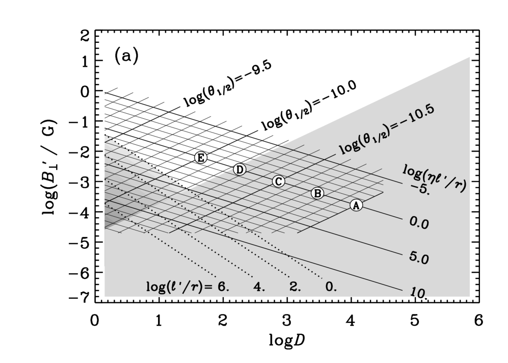
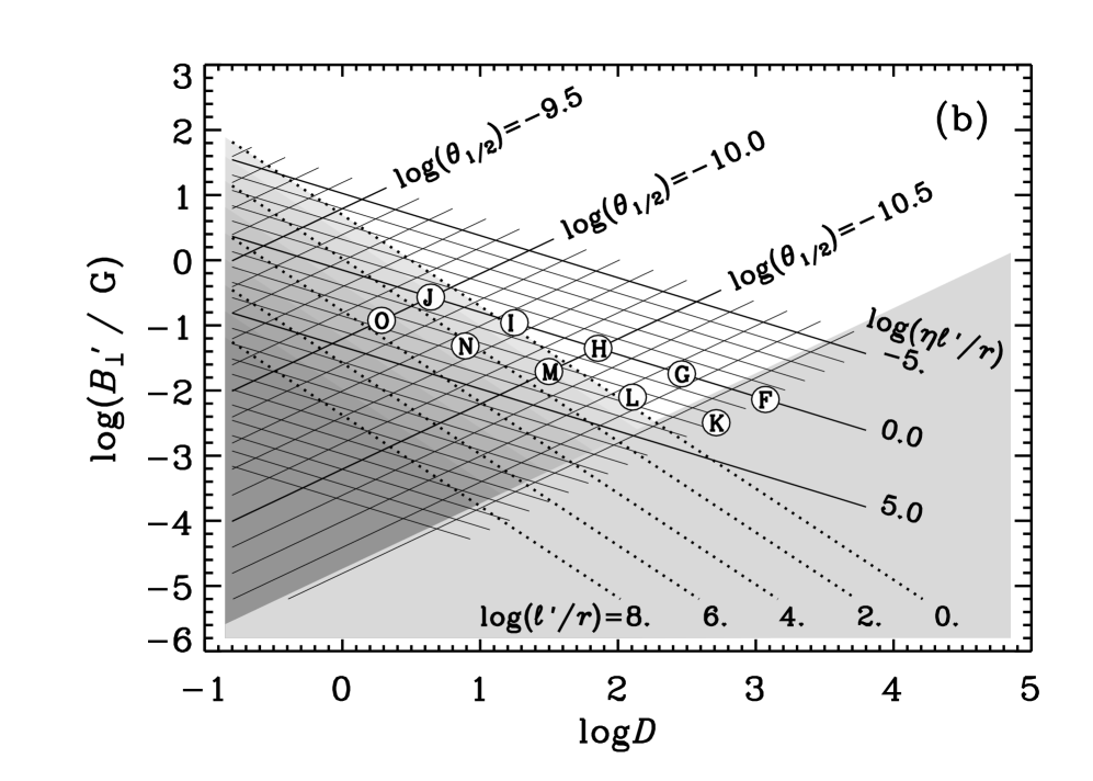
Figure 4: Magnetic field–Doppler factor parameter space for models fitting the radio intensity of the IDV core of PKS 0405-385 with $\nu_{1}=10^{9.1}$ Hz and (a) $\nu_{c}=10^{11}$ Hz or (b) $\nu_{c}=10^{13.65}$ Hz, i.e. giving the left and right solid curves in Fig. 1. The two sets of solid curves labeled by $\log(\eta\ell^{\prime}/r)$ and $\log(\theta_{1/2})$ are given by equations (20) and (21) plotted using $\theta_{1/2}$ and $(\eta\ell^{\prime}/r)$, respectively, as the parameter, and are used to obtain the values of $\theta_{1/2}$ and $(\eta\ell^{\prime}/r)$ for any combination of $B_{\perp}$ and $D$ that are necessary to give the required radio spectrum. The shaded region on the right shows where the energy losses are dominated by IC on the CMBR and corresponds to equation (29), and the shaded regions on the left show where the energy losses are dominated by IC on synchrotron photons and correspond to equation (30) for various values of $\log(\ell^{\prime}/r)$ indicated. Fifteen models, i.e. combinations of $B_{\perp}$, $D$, $\theta_{1/2}$ and $(\eta\ell^{\prime}/r)$, which will be discussed later are labeled A to O.

If one allows the relativistic particle energy density to exceed the magnetic energy density, then very low Doppler factors are possible. However, if the equipartition factor is greater than unity, this would be unstable. It is therefore probably unrealistic for the relativistic particles to be too far from equipartition with the magnetic field, and so one should perhaps take more seriously results corresponding to $\eta=1$, which I shall assume in what follows. Nevertheless, IDV is truly a time-dependent problem, and episodes with $\eta>1$ are not ruled out completely.

4.1 Avoiding Compton catastrophes

If electrons are injected with jet-frame Lorentz factor $\gamma^{\prime}$ then the presence of dense radiation fields provides target photons for inverse Compton scattering, and the generation of components in the SED at X-ray and gamma-ray frequencies which may or may not exceed observed X-ray flux and gamma-ray limit. If the electrons are accelerated in a quasi-continuous process such as diffusive shock acceleration by non-relativistic or mildly-relativistic shocks, then the presence of dense radiation fields may lead to excessive energy losses and prevent the electrons reaching the Lorentz factor required to fit the observed radio spectrum. In either case, these effects may occur wherever the photon energy density in the emission region becomes comparable to or exceeds the energy density in the magnetic field.

In addition to the synchrotron emission itself, I shall assume that emission region is sufficiently far along the jet that the only other non-negligible field for inverse-Compton scattering is the cosmic microwave background radiation (CMBR). If the emission region were close to the central engine then accretion disk radiation, broad line cloud emission, and torus infrared emission could also play a role (Donea & Protheroe 2002).

The average jet-frame energy density of the synchrotron emission inside the emission region can be estimated for given $\ell^{\prime}/r$ values from the observed intensity $I_{\nu}$ corresponding to $\nu^{2}F_{\nu}$ plotted as the solid curves in Fig. 1. The energy density in the jet frame is given by

$$\langle U^{\prime}_{\rm syn}(\ell^{\prime}/r,\theta_{1/2})\rangle=D^{-4}\langle U_{\rm syn}(\ell^{\prime}/r,\theta_{1/2})\rangle$$ (22)

where

$$\langle U_{\rm syn}(\ell^{\prime}/r,\theta_{1/2})\rangle$$

$$= {4\pi\over c}\int M[\ell^{\prime}/r,\tau_{\nu}(\nu)]I_{\nu}(\nu,\theta_{1/2})d\nu,$$ (23)

$\tau_{\nu}(\nu)\approx(\nu_{1}/\nu)^{5/3}$ from Fig. 2, and $M[\ell^{\prime}/r,\tau_{\nu}(\nu)]=\langle U^{\prime}_{\nu^{\prime}}\rangle/(4\pi I^{\prime}_{\nu^{\prime}}/c)$ given in Fig. 3. The main contribution to the energy density for the spectrum fitted to the radio observations of the IDV core in PKS 0405-385 comes from frequencies near to $\nu_{c}$ since this is where the SED, $\nu F_{\nu}$, peaks. This spectrum is optically thin near $\nu_{c}$ and so I may make the approximation

$$\langle U_{\rm syn}(\ell^{\prime}/r,\theta_{1/2})\rangle$$

$$\approx M(\ell^{\prime}/r,\tau_{\nu}\ll 1){4\pi\over c}\int I_{\nu}(\nu,\theta_{1/2})d\nu,$$

$$\approx M(\ell^{\prime}/r,\tau_{\nu}\ll 1)g(\nu_{1},\nu_{c})F_{1}\theta_{1/2}^{-2},$$ (24)

where

$$g(\nu_{1},\nu_{c})={4\over c}\int{F_{\nu}(\nu)\over F_{\nu}(\nu_{1})}d\nu.$$ (25)

For the spectra shown by the solid curves in Fig. 1, $M(1,\tau_{\nu}\!\ll\!1)g(10^{9.1}$Hz$,10^{11}$Hz$)=45.14$ cm^-1sr Hz and $M(1,\tau_{\nu}\!\ll\!1)g(10^{9.1}$Hz$,10^{13.65}$Hz$)=1.47\times 10^{5}$ cm^-1sr Hz.

In the rest frame of the host galaxy the CMBR would have had temperature $(1+z)T_{0}$, where $T_{0}=2.735$ K, and would have been isotropic. I shall distinguish between the Doppler factor for boosting from the jet frame to the host galaxy frame, $\delta$, and the Doppler factor for boosting from the jet frame to the observer frame, $D=\delta/(1+z)$. In the jet frame, the black body temperature would depend on the angle $\psi^{\prime}$ with respect to the jet axis at which an observer in the jet frame looks

$$T^{\prime}(\psi^{\prime})={(1+z)T_{0}\over\Gamma(1-\beta_{j}\cos\psi^{\prime})}$$ (26)

where $\beta_{j}c$ is the jet velocity as measured in the host galaxy frame, $\Gamma=(1-\beta_{j}^{2})^{-1/2}$ is its Lorentz factor, and is given by $\Gamma=(\delta^{2}+1)/(2\delta)$ for the case of observation of the AGN jet at angle $\theta=0$ to its axis. The energy density of the CMBR in the jet frame is then

$$U^{\prime}_{\rm CMBR} = {(1+z)^{4}aT_{0}^{4}\over 4\pi}\oint{d\Omega^{\prime}\over[\Gamma(1-\beta_{j}\cos\theta^{\prime})]^{4}}$$ (27)

$$= {4\over 3}\Gamma^{2}(1+z)^{4}aT_{0}^{4}.$$

where $a=4\sigma/c$ and $\sigma$ is the Stefan-Boltzmann constant. Note that whereas the jet frame energy density of synchrotron radiation decreases with assumed Doppler factor, the energy density of the CMBR increases with assumed Doppler factor. This means that the Compton catastrophe can not be avoided by using an arbitrarily large Doppler factor. In fact, very high Doppler factors will result in a Compton catastrophe due to inverse-Compton scattering on the CMBR. This has important consequences which I shall address next, and in subsequent sections.

For efficient synchrotron radiation to take place the energy density in the magnetic field should exceed the energy density in the radiation field

$${3\over 2}{{B^{\prime}}_{\perp}^{2}\over(8\pi)}>\left[D^{-4}\langle U_{\rm syn}(\ell^{\prime}/r)\rangle+{4\over 3}\Gamma^{2}(1+z)^{4}aT_{0}^{4}\right].$$ (28)

Since the synchrotron photon energy density is large in the regime of low Doppler factors, while the CMBR energy density is large in the regime of high Doppler factors, I shall obtain separately the minimum magnetic field required in each case. For PKS 0405-385 being viewed along the jet axis, and using the approximation $\Gamma\approx(1+z)D/2$, valid for $\Gamma\gg 1$, the jet-frame energy density of the magnetic field is less than that of the CMBR when

$$B^{\prime}_{\perp}<(4/3)\sqrt{a\pi}(1+z)^{3}T_{0}^{2}D$$ (29)

and this is independent of all model parameters except $D$. This case is shown by the shaded area on the right in Figs. 4(a)–(b).

In the case of synchrotron photons as targets for inverse Compton scattering, i.e. the synchrotron self-Compton (SSC) process, inverse Compton losses dominate when

$${B^{\prime}}_{\perp} < 4(\pi/3)^{1/2}D^{-2}\langle U_{\rm syn}(\ell^{\prime}/r,\theta_{1/2})\rangle^{1/2}.$$ (30)

Because in this case the photon energy density depends on $\theta_{1/2}$ and $\ell^{\prime}/r$, in addition to $D$, the boundary between models ($D,B^{\prime}_{\perp}$) is parametrized by substituting $D$ from equation (19) into equation (30) and solving for $B^{\prime}_{\perp}$ as a function of the parameters, and then using equation (19) to obtain $D$ as a function of the parameters. The resulting minimum value of $B^{\prime}_{\perp}$ is plotted against $D$ in Figs. 4(a)–(b) for various values of $\ell^{\prime}/r$ as the dotted lines (labeled by $\ell^{\prime}/r$) bounding the shaded areas on the left.

The gyroradius, $r^{\prime}_{g}=\gamma^{\prime}c/(B^{\prime}_{\perp}\omega_{B})$ must be much smaller than the radius $r$ of the cylinder and so this provides, in principle, an additional lower limit to $B^{\prime}_{\perp}$. However, this limit is well below the lower limit from equation (28) already plotted, and therefore does not further constrain the models.

Fifteen potential models which will be discussed later, i.e. combinations of $B_{\perp}$, $D$, $\theta_{1/2}$ and $(\eta\ell^{\prime}/r)$, are labeled as A to O in Fig. 4. Before proceeding, we should check if any of these models is ruled out by being optically thick to Thomson scattering. The Thomson optical depth is $\tau_{T}=\ell^{\prime}n_{e}^{\prime}\sigma_{T}$ where $\sigma_{T}$ is the Thomson cross section. Taking $n_{e}^{\prime}$ from equation (15) with $\gamma^{\prime}$ from equation (16) I obtain

$$\tau_{T}=2.11\times 10^{24}{B^{\prime}}_{\perp}^{2}D\theta_{1/2}^{3}\left(\eta{\ell^{\prime}\over r}\right).$$ (31)

For the fifteen potential models the Thomson optical depth ranges from $\tau_{T}=7.04\times 10^{-13}$ (Model A) to $\tau_{T}=1.83\times 10^{-5}$ (Model O), and so Thomson scattering can be neglected in this case.

5 Calculating the Spectral Energy Distribution

I shall consider the following three emission processes: synchrotron radiation (syn), inverse Compton scattering of synchrotron photons (SSC), and inverse Compton scattering of CMBR photons (ICM). Assuming the inverse Compton scattering is in the Thomson regime, the rate of energy loss by either process is

$${dE^{\prime}\over dt^{\prime}}=-{4\over 3}\sigma_{T}c{\gamma^{\prime}}^{2}U^{\prime}$$ (32)

where $U^{\prime}=U^{\prime}_{B}$ for synchrotron losses, $U^{\prime}=\langle U^{\prime}_{\rm syn}\rangle$ for SSC losses and $U^{\prime}=U^{\prime}_{\rm CMBR}$ for inverse-Compton losses on the CMBR. The fraction of emitted radiation by each process is then

$$f_{\rm syn} = U^{\prime}_{B}/(U^{\prime}_{B}+\langle U^{\prime}_{\rm syn}\rangle+U^{\prime}_{\rm CMBR})$$ (33)

$$f_{\rm SSC} = \langle U^{\prime}_{\rm syn}\rangle/(U^{\prime}_{B}+\langle U^{\prime}_{\rm syn}\rangle+U^{\prime}_{\rm CMBR})$$ (34)

$$f_{\rm ICM} = U^{\prime}_{\rm CMBR}/(U^{\prime}_{B}+\langle U^{\prime}_{\rm syn}\rangle+U^{\prime}_{\rm CMBR}).$$ (35)

This does not mean, however, that the observed energy flux for the inverse-Compton scattered CMBR is in this ratio to the other two components because, whereas the synchrotron emission and SSC emission is isotropic in the jet frame, the inverse-Compton scattering of the CMBR is not because of the anisotropy of the CMBR in this frame. One may well expect strong peaks in the SED due to inverse-Compton scattering for models close to or within the shaded areas in Figs. 4(a)–(b). Slysh (1992) also noted that gamma-ray emission may occur in IDV sources.

5.1 Synchrotron radiation

The intensity of synchrotron emission in direction $\theta=0$ in the observer frame is simply given by

$$I_{\nu}^{\rm syn}(\nu,\theta=0)=D^{3}S^{\prime}_{\nu^{\prime}}(\nu/D)\{1-\exp[-\tau^{\prime}_{\nu^{\prime}}(\nu/D)]\}$$ (36)

where $\tau^{\prime}_{\nu^{\prime}}(\nu/D)=\alpha^{\prime}_{\nu^{\prime}}(\nu/D)\ell^{\prime}$.

5.2 Inverse Compton scattering of synchrotron photons (SSC)

In the present paper I shall assume that we view the emission emitted at angle $\theta^{\prime}=\theta=0$ to the jet axis. The electrons are assumed to be isotropic and mono-energetic in the jet frame, and have Lorentz factor $\gamma^{\prime}=\gamma_{1}/D$, and velocity $\beta^{\prime}c=(1-1/{\gamma^{\prime}}^{2})^{1/2}c$. For simplicity, I shall also take the synchrotron target photons to be isotropic in the jet frame, while using the results from Section 3 to normalize their spectrum.

For isotropic target photons in the jet frame with frequency $\nu^{\prime}_{0}$, the frequency of the scattered photons range between 0 and $4{\gamma^{\prime}}^{2}\nu^{\prime}_{0}$. The jet-frame SSC emissivity (erg cm^-3 s^-1 sr^-1 Hz^-1) is then

$$j_{\nu^{\prime}}^{\rm\prime\,SSC}={n_{e}^{\prime}3h\nu^{\prime}\sigma_{T}c\over 4{\gamma^{\prime}}^{2}}\int_{\nu^{\prime}/4{\gamma^{\prime}}^{2}}^{\infty}{d\nu^{\prime}_{0}\over\nu^{\prime}_{0}}\langle n^{\prime}_{\rm syn}(\nu^{\prime}_{0})\rangle f_{\rm IC}(x)$$ (37)

where

$$\langle n^{\prime}_{\rm syn}(\nu_{0}^{\prime})\rangle={M(\ell^{\prime}/r,\tau_{\nu}\ll 1)\over h\nu^{\prime}_{0}c}I_{\nu^{\prime}}^{\rm\prime syn}(\nu_{0}^{\prime},\theta^{\prime}=0)$$ (38)

is the average jet-frame synchrotron specific photon number density (photons cm^-3 sr^-1 Hz^-1), $x=\nu^{\prime}/4{\gamma^{\prime}}^{2}\nu_{0}^{\prime}$ and $f_{\rm IC}(x)=2x\ln x+x+1-2x^{2}$ (Blumenthal and Gould 1970), giving

$$I_{\nu^{\prime}}^{\rm\prime\,SSC}(\nu^{\prime};\theta^{\prime}\!=\!0)=\ell^{\prime}j_{\nu^{\prime}}^{\rm\prime\,SSC}.$$ (39)

Finally, this is Doppler boosted to the observer frame

$$I_{\nu}^{\rm SSC}(\nu;\theta\!=\!0)=D^{3}I_{\nu^{\prime}}^{\rm\prime\,SSC}(\nu/D;\theta^{\prime}\!=\!0)$$ (40)

5.3 Inverse-Compton scattering of the CMBR: gamma ray production

In the jet frame, the black body temperature would depend on the angle $\theta_{0}^{\prime}$ with respect to the jet axis at which the CMBR target photons propagate

$$T^{\prime}(\theta_{0}^{\prime})={(1+z)T_{0}\over\Gamma(1+\beta_{j}\cos\theta_{0}^{\prime})},$$ (41)

such that their specific photon number density (photons cm^-3 sr^-1 Hz^-1) is

$$n^{\prime}_{\rm CMBR}(\nu^{\prime}_{0},\theta_{0}^{\prime})={2h{\nu^{\prime}_{0}}^{2}/c^{3}\over\exp[h{\nu^{\prime}_{0}}/kT^{\prime}(\theta_{0}^{\prime})]-1}.$$ (42)

For target photons in the jet frame with frequency $\nu^{\prime}_{0}$ propagating at angle $\theta_{0}^{\prime}$ to the jet axis, the frequencies of the photons scattered by electrons propagating parallel to the jet axis are uniformly distributed between 0 and $\nu^{\prime}_{\rm max}(\nu^{\prime}_{0},\theta_{0}^{\prime})=2{\gamma^{\prime}}^{2}\nu^{\prime}_{0}(1-\beta^{\prime}\cos\theta_{0}^{\prime})$ in the approximation that the scattered photons are isotropic in the electron rest frame. The jet-frame emissivity (erg cm^-3 s^-1 sr^-1 Hz^-1) for IC on the CMBR in the jet direction is then

$$j_{\nu^{\prime}}^{\rm\prime\,ICM}(\theta^{\prime}\!=\!0) = {n_{e}^{\prime}h\nu^{\prime}\sigma_{T}c}\int_{-1}^{1}{d\cos\theta_{0}^{\prime}\over 2}(1-\beta^{\prime}\cos\theta_{0}^{\prime})$$ (43)

$$\hskip 20.00003pt\int_{{\nu^{\prime}}_{0}^{\rm min}(\theta_{0}^{\prime})}^{\infty}{d\nu^{\prime}_{0}}{n^{\prime}_{\rm CMBR}(\nu^{\prime}_{0},\theta_{0}^{\prime})\over\nu^{\prime}_{\rm max}(\nu^{\prime}_{0},\theta_{0}^{\prime})}$$

where ${\nu^{\prime}}_{0}^{\rm min}(\theta_{0}^{\prime})=\nu^{\prime}/2{\gamma^{\prime}}^{2}(1-\beta^{\prime}\cos\theta_{0}^{\prime})$. Finally,

$$I_{\nu^{\prime}}^{\rm\prime\,ICM}(\nu^{\prime};\theta^{\prime}\!=\!0) = \ell^{\prime}j_{\nu^{\prime}}^{\rm\prime\,ICM}(\theta^{\prime}\!=\!0),$$ (44)

$$I_{\nu}^{\rm ICM}(\nu;\theta\!=\!0) = D^{3}I_{\nu^{\prime}}^{\rm\prime\,ICM}(\nu/D;\theta^{\prime}\!=\!0).$$ (45)

6 Discussion

The angular radius inferred by Kedziora-Chudczer et al. (1997) is $\theta_{1/2}\approx 1.5\times 10^{-11}$ rad, i.e. $\log(\theta_{1/2})=-10.83$. Examining the parameter space for $\nu_{c}=10^{9.1}$ in Fig. 4(a), one sees that all models with this angular radius lie well inside the region where IC on the CMBR dominates the energy losses of electrons. For $\eta=1$ (equal energy density in magnetic field and relativistic electrons) and $\ell^{\prime}/r=1$ this would correspond to a point roughly mid-way between models A and B, and would require a Doppler factor of $D\sim 5000$. By choosing $\ell^{\prime}/r>1$ one may reduce the Doppler factor, but unrealistically large $\ell^{\prime}/r$ values are needed to reduce $D$ by a large factor. To reduce the Doppler factor to a reasonable value, i.e. $D<100$, would require the angular diameter to be larger by only a factor of $\sim 5$ which, as discussed earlier, I believe is quite possible (for an angular diameter larger by a factor of 10, even $D\sim 10$ is possible).

6.1 Spectral energy distribution

Because of the dominance of IC losses on the CMBR for models A–D, one would expect the SSC peak at gamma-ray energies in the SED to exceed the synchrotron peak for these models. The SEDs have been calculated for models A–E and are shown in Fig. 5(a) and, as expected, show strong gamma-ray emission for models A–D. Non-contemporaneous X-ray and gamma-ray data are shown, and may be used with caution as upper limits. I have added to Fig. 5 the sensitivity of the IBIS gamma-ray detector on INTEGRAL (Parmar et al. 2002), and the expected sensitivities of GLAST (Gehrels and Michelson 1999), and HESS (Hofmann et al. 2001) and CANGAROO III (Enomoto et al. 2002), the last two being southern hemisphere atmospheric Cherenkov telescopes nearing completion. Taking the X-ray data as an upper limit does not rule out any of these models. However, the EGRET upper limit obtained from figure 3 of Hartman et al. (1999) appears to exclude models A–C but be consistent with models D–E (note, however, that the EGRET data are not contemporaneous with the IDV data). Models D–E have $\theta_{1/2}\approx 6\times 10^{-11}$–$10^{-10}$ rad and $D\approx 180$–40, respectively.

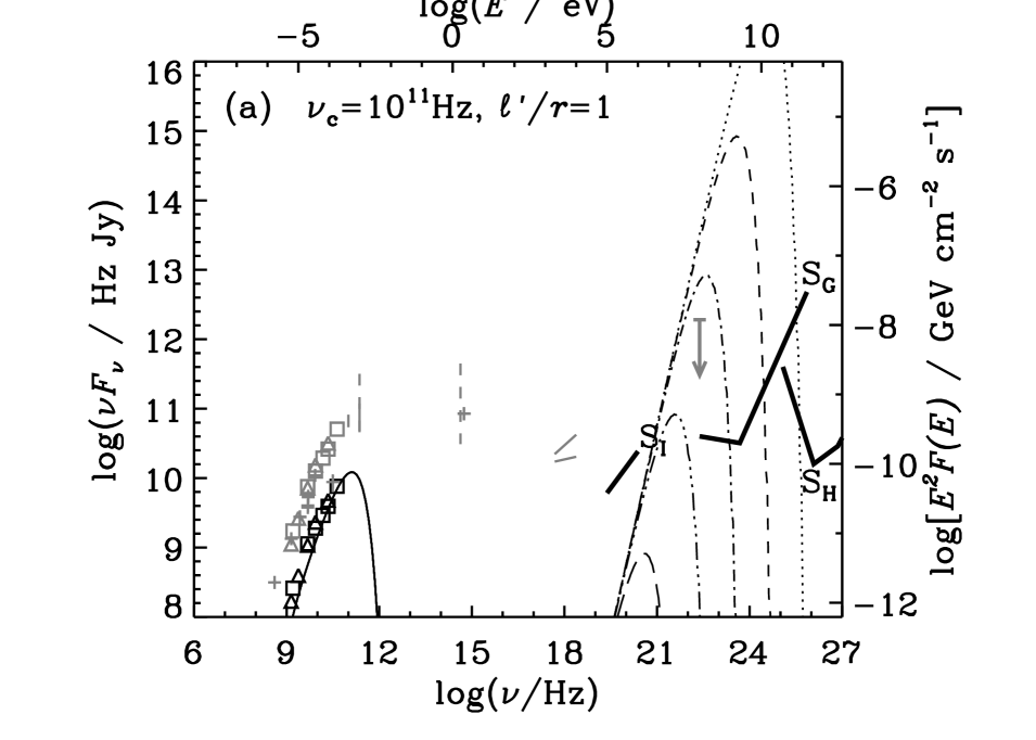
Figure 5: SED of IDV core of PKS 0405-385 obtained from observed fluxes assuming flux fraction $S_{c}$ only for the ACTA/VLA data as in Fig. 1. Data additional to those shown in Fig. 1: X-ray data at $\sim 10^{18}$ Hz – 1997 ASCA fluxes (L. Kedziora-Chudczer personal communication 1999); gamma-ray data – EGRET upper limit (Hartman et al. 1999). Sensitivities of the IBIS instrument on INTEGRAL (S_I), GLAST (S_G) and HESS (S_H) indicated (the expected sensitivity of CANGAROO III is similar to that of HESS). The calculated SED is shown for various models with the synchrotron component as the solid curve on the left, the SSC component in the middle (when present) and the scattered CMBR component on the right. (a) The SED for models A–E in Fig. 4(a) with $\nu_{c}=10^{9.1}$, $\eta=1$ and $(\ell^{\prime}/r)=1$: A – dotted curves, B – short dashed curves, C – chain curves, D – triple-dot dashed curves, E – long dashed curves.

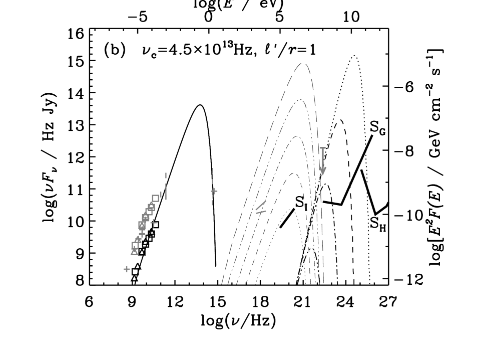
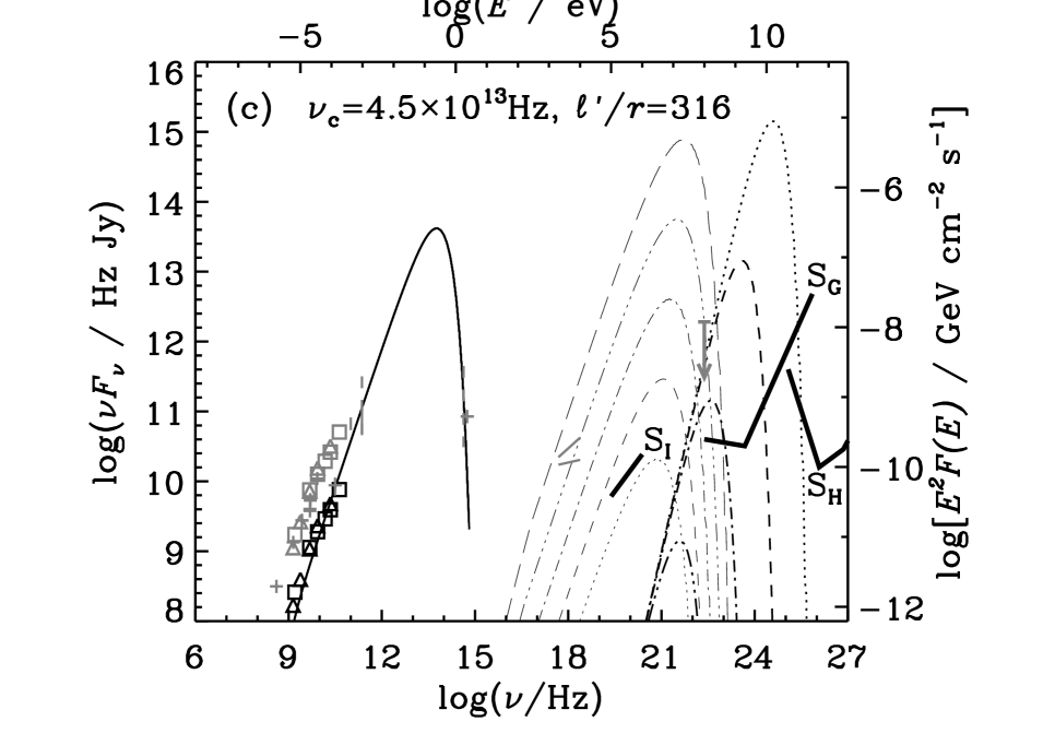
Figure 6: continued

(b) The SED for models F–J in Fig. 4(b) with $\nu_{c}=10^{13.65}$, $\eta=1$ and $(\ell^{\prime}/r)=1$: F – dotted curves, G – short dashed curves, H – chain curves, I – triple-dot dashed curves, J – long dashed curves. (c) The SED for models K–O in Fig. 4(b) with $\nu_{c}=10^{13.65}$, $\eta=1$ and $(\ell^{\prime}/r)=316$: K – dotted curves, L – short dashed curves, M – chain curves, N – triple-dot dashed curves, O – long dashed curves.

As expected from equation 20, increasing $\nu_{c}$ from $10^{11}$ Hz to $10^{13.65}$ Hz reduces $D$ by a factor of 10 if one keeps all other parameters fixed (note, however, that this reduction in $D$ is accompanied by an increase in $B^{\prime}_{\perp}$). This is clearly seen in Fig. 4(b) which is for $\nu_{c}=10^{13.65}$ Hz, and thereby presents more opportunity for obtaining reasonable values of $D$. For $\eta=1$ and $\ell^{\prime}/r=1$, models F–J have the same angular radius range ($10^{-11}$–$10^{-10}$ rad) as models A–E, but with considerably lower Doppler factors, and these models range from being in the IC on CMBR dominated regime (model F – expect highest gamma-ray flux, lowest SSC flux) to being in the SSC dominated regime (model J – expect highest SSC flux, lowest gamma-ray flux). The calculated SEDs for models F–J are shown in Fig. 5(b) and show the trends expected. Possibly models I and J may be ruled out by the X-ray data taken as an upper limit (note, however, that the X-ray data is not contemporaneous with the IDV data). Models F–I predict high gamma-ray fluxes from MeV energies to 100 GeV energies, depending on model, which could be tested observationally by INTEGRAL, GLAST, HESS and CANGAROO III. Models F–I have $\theta_{1/2}\approx 10^{-11}$–$6\times 10^{-11}$ rad and $D\approx 1000$–20, respectively.

As also expected from equation 20, increasing $\ell^{\prime}/r$ from 1 to 316 results in a reduction in $D$ by a factor of $\sim 2$ (plus a reduction in $B^{\prime}_{\perp}$) if one keeps all other variables fixed. Models K–O in Fig. 4(b) have all other parameters the same as models F–J, and the resulting SEDs are shown in Fig. 5(c). Because of the reduction in synchrotron photon energy density associated with $\ell^{\prime}/r\gg 1$, although not identical, the SEDs of models K–O are qualitatively similar to those of models F–J, with model O being ruled out by both the gamma-ray limit and the X-ray data, although again I note that these data are not contemporaneuos with the IDV data. Models K–N have $\theta_{1/2}\approx 10^{-11}$–$6\times 10^{-11}$ rad and $D\approx 400$–8. Model M, having $\theta_{1/2}$ only $\sim 5$ times that assumed by Kedziora-Chudczer et al. (1997) has a Doppler factor of $\sim 30$, and lower Doppler factors are possible with, for example even larger $\ell^{\prime}/r$. Bearing in mind that no attempt has been made to fit the (non-contemporaneous) X-ray and gamma-ray data, and that a simple mono-energetic electron spectrum has been used, it seems that models which are able to fit the IDV radio data tend to predict observable fluxes of X-ray, and/or gamma ray emission at sub-GeV and/or $\sim$10 GeV energies. Use of a more sophisticated electron spectrum is unlikely to alter this conclusion. Hence, it may well be profitable for space gamma ray telescopes such as INTEGRAL and GLAST, and southern hemisphere atmospheric Cherenkov telescopes such as HESS and CANGAROO III to look for emission from PKS 0405-385 and other extreme IDV radio galaxies.

6.2 Variability

The rapid intra-day variability in PKS 0405-385 is almost certainly due to interstellar scintillation effects. The radio flux does, however, also vary on longer timescales – 10 per cent change in 2 months in July 1996 (corresponding to $\sim 1$ yr for 50 per cent change), and has very intense for periods of about a month (Kedziora-Chudczer et al. 1997).

A mechanism that may cause such variability would be the emission region moving along the jet and passing a region where external factors cause compression/expansion of the emission region, increasing/decreasing the magnetic field, and causing adiabatic acceleration/deceleration of relativistic charged particles, thereby affecting the observed intensity. Change can also occur as a result of the emission region passing through a bend in the jet causing, amongst other things, a change in viewing angle with respect to the motion of the emission region, and hence a change in Doppler factor.

For the examples above, the observer-frame variability time depends on the geometry of the emission region (see, e.g., Protheroe 2002) and, for viewing the assumed cylindrical emission region along its axis, is at least $\ell^{\prime}/(2Dc)$. In general, arbitrarily low Doppler factors are possible for arbitrarily high $\ell^{\prime}/r$. However, in this case this is clearly at the expense of having a time scale for variability which may be unreasonably large, and of course also requires the jet to be extremely well collimated over the length of the emission region.

Alternatively a shock may pass through the emission region compressing the magnetic field and accelerating particles – a pre-existing mono-energetic population of relativistic particles will receive an energy boost by a factor of $\sim{\gamma^{\prime}}_{\rm shock}^{2}$ and acquire a power-law tail as a result of diffusive shock acceleration. In the case of a plane shock moving at jet-frame speed $\beta^{\prime}_{\rm shock}c$ along the jet (see, e.g. Protheroe 2002), the observer-frame variability time in our case ($\theta^{\prime}=0$) is at least

$$t_{\rm var,shock}=D^{-1}\left({\ell^{\prime}\over 2c}\right)\left|1-{1\over\beta^{\prime}_{\rm shock}}\right|$$ (46)

which is longer (shorter) than $\ell^{\prime}/(2Dc)$ if $\beta^{\prime}_{\rm shock}$ is less than (greater than) 0.5 for a forward-moving shock.

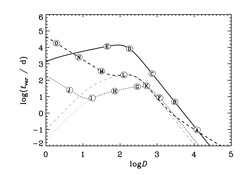
Figure 7: Observer-frame variability time (thick curves) and energy-loss time (thin curves) vs. Doppler factor, $D$, for: $\nu_{c}=10^{9.1}$, $\eta=1$ and $(\ell^{\prime}/r)=1$ (solid curves); $\nu_{c}=10^{13.65}$, $\eta=1$ and $(\ell^{\prime}/r)=1$ (dotted curves); and $\nu_{c}=10^{13.65}$, $\eta=1$ and $(\ell^{\prime}/r)=316$ (dashed curves). The variability times for models A–O are indicated.

Except for a point-like emission region following a bent or helical trajectory such that the Doppler boosting factor, changes rapidly with time, the variability time can not be shorter than the observer-frame energy-loss time scale, $D^{-1}E^{\prime}/(dE^{\prime}/dt^{\prime})$. This is easily obtained from equation (32) and is plotted (thin curves) against Doppler factor in Fig. 7 for the following cases: $\nu_{c}=10^{9.1}$, $\eta=1$ and $(\ell^{\prime}/r)=1$ (solid curves) $\nu_{c}=10^{13.65}$, $\eta=1$ and $(\ell^{\prime}/r)=1$ (dotted curves); and $\nu_{c}=10^{13.65}$, $\eta=1$ and $(\ell^{\prime}/r)=316$ (dashed curves). As noted above, the variability time will in general be longer than the energy-loss time scale due to the dimensions of the emission region. For the present geometry and viewing angle, I take the variability time to be

$$t_{\rm var}=D^{-1}\left\{\left({\ell^{\prime}\over 2c}\right)^{2}+\left[{E^{\prime}\over(dE^{\prime}/dt^{\prime})}\right]^{2}\right\}^{1/2},$$ (47)

but one should note that in the case of shock excitation that it can be longer than this for $\beta^{\prime}_{\rm shock}<0.5$, or as short as $D^{-1}E^{\prime}/(dE^{\prime}/dt^{\prime})$ if $\beta^{\prime}_{\rm shock}\to 1$. In Fig. 7, I have also plotted $t_{\rm var}$ vs. $D$ for the same three cases, and the values for models A–O are indicated by the letters. Of the models with Doppler factors less than $\sim 10^{3}$, models C–E give variability times $\sim 1$–30 years. Models F–J give variability times of $\sim 1$ week to $\sim$ month, and are quite compatible with the long-term variability observed for PKS 0405-385. Models K–O, with larger $\ell^{\prime}/r$, give variability times of $\sim 1$ month to $\sim 100$ years, with model M having $t_{\rm var}\approx 1$ year.

7 Conclusion

To obtain low Doppler factors, without invoking extreme variations from equipartition, requires a larger angular diameter for the IDV core of PKS 0405-385 than the $\sim 6$ micro-arcsec assumed by Kedziora-Chudczer et al. (1997) corresponding to a distance of $\sim 500$ pc to the ionized material responsible for the interstellar scintillation. A further reduction in the minimum Doppler factor needed to avoid the Compton Catastrophe can be obtained by having optically thin IDV core emission, preferably originating from a region elongated along the jet, and observing it at a small viewing angle with respect to the jet axis. An angular diameter a factor of $\sim 2$–4 larger than assumed by Kedziora-Chudczer et al. (1997) and Walker (1998) corresponds roughly to models D, H–I and M–N, all of which are allowed by the present data, and have Doppler factors $\sim 200$, 80–20 and 30–8, respectively. Interstellar scintillation screen distances as small as 20 pc, possibly associated with material in the local bubble, have previously been invoked to explain IDV in J1819+3845 (Dennett-Thorpe & de Bruyn 2000, 2002). By using a distance of 20 pc, even lower Doppler factors could easily fit the observations.

In conclusion, if one observes optically thin emission along a long narrow emission region, the average energy density in the emission region can be significantly lower than $(4\pi/c)\int I_{\nu}d\nu$. If one takes into account the uncertainty in the distance to the ionized clouds responsible for interstellar scintillation causing rapid IDV in PKS 0405-385 the brightness temperature could be as low as $\sim 10^{13}$ K, or lower, at 5 GHz. The radio spectrum can be fit by $I_{\nu}\propto\nu^{1/3}$ expected if the emission is optically thin and the electrons are mono-energetic, or have a minimum Lorentz factor whose critical frequency is well above the frequency range of interest. Such a spectrum would occur naturally in models in which $e^{\pm}$ are produced as secondaries of interactions of protons, e.g. by Bethe-Heitler pair production, or through $\pi^{\pm}\to\mu^{\pm}\to e^{\pm}$ decay following collisions of with matter or low-energy target photons (pion photoproduction) by protons, or by neutrons themselves produced in pion photoproduction interactions (e.g. $p\gamma\to n\pi^{+}$) perhaps closer to the central engine. The combination of all these factors enables the Compton catastrophe to be avoided, and also predicts that X-ray and gamma-ray emission at observable flux levels should be expected from compact cores of extreme IDV sources such as PKS 0405-385.

References

- [1] Beckert T., Kraus A., Krichbaum T.P., Witzel A., Zensus J.A., 2001, in Particles and Fields in Radio Galaxies, R. A. Laing and K. M. Blundell, eds., ASP Conf. Series, 250, 147
- [2] Blumenthal G.R, Gould R.J., 1970, Rev. Mod. Phys., 42, 237
- [3] Cimo G., Beckert T., Krichbaum T.P., Fuhrmann L., Kraus A., Witzel A., Zensus J.A., 2002, PASA, 19, 10
- [4] Dennett-Thorpe J., de Bruyn A.G., 2000, ApJ, 529, L65
- [5] Dennett-Thorpe J., de Bruyn A.G., 2002, Nature, 415, 57
- [6] Donea A.-C., Protheroe R.J., 2002, PASA, 19, 39
- [7] Enomoto R. et al., 2002, Astropart. Phys., 16, 235
- [8] Gomez G.C., Benjamin R.A., Cox D.P., 2001, AJ, 122, 908
- [9] Gehrels N., Michelson P., 1999, Astropart. Phys., 11, 277
- [10] Hartman R.C. et al., 1999, ApJS, 123, 79
- [11] Hofmann W. et al., 2001, Proc. 27th Int. Cosmic Ray Conf., eds. M. Simon et al., pub. Copernicus Gesellschaft, Katlenburg-Lindau, vol. 7, p. 2785
- [12] Kardashev N.S., 2000, Astron. Reports, 44, 719
- [13] Kedziora-Chudczer L., Jauncey D.L., Wieringa M.H., Walker M.A., Nicolson G.D., Reynolds J.E., Tzioumis A.K., 1997, ApJ, 490, L9.
- [14] Kedziora-Chudczer L.L., Jauncey D.L., Wieringa M.H., Tzioumis A.K., Reynolds J.E., 2001, MNRAS, 325, 1411
- [15] Kellermann K.I., Paulini-Toth I.I.K., 1969, ApJ, 155, L71
- [16] Krichbaum T.P., Kraus A., Fuhrmann L., Cimo G., Witzel A., 2002, PASA, 19, 14
- [17] Parmar A. et al., 2002, Proceedings SPIE 4851, X-ray and gamma-ray telescopes and instruments for astronomy, August 2002
- [18] Protheroe R.J., 2002, PASA, 19, 486
- [19] Rybicki R.B., Lightman A.P., 1979, Radiative Processes in Astrophysics, Wiley: New York
- [20] Slysh V.I., 1992, ApJ, 391, 453
- [21] Taylor J.H., Cordes J.M., 1993, ApJ, 411, 674
- [22] Tornikoski M., Valtaoja E., Teraesranta H., Karlamaa K., Lainela M., Nilsson K., Kotilainen J., Laine S., Laehteenmaeki A., Knee L.B.G., Botti, L.C.L., 1996, A&AS, 116, 157
- [23] Wagner S.J., Witzel A., 1995, ARA&A, 33, 163
- [24] Walker M.A., 1998, MNRAS, 294, 307