The Origin of Subdwarf B Stars (II)

Abstract

We have carried out a detailed binary populations synthesis (BPS) study of the formation of subdwarf B (sdB) stars and related objects (sdO, sdOB stars) using the latest version of the BPS code developed by Han et al. (1994, 1995a, 1995b, 1998, 2001). We systematically investigate the importance of the five main evolutionary channels in which the sdB stars form after one or two common-envelope (CE) phases, one or two phases of stable Roche-lobe overflow (RLOF) or as the result of the merger of two helium white dwarfs (WD) (see Han et al. 2002, Paper I). Our best BPS model can satisfactorily explain the main observational characteristics of sdB stars, in particular their distributions in the orbital period – minimum companion mass ($\log P$ - $M_{\rm comp}$) diagram and in the effective temperature – surface gravity ($T_{\rm eff}$ - $\log g$) diagram, their distributions of orbital period, $\log(g\theta^{4})$ ($\theta=5040\,{\rm K}/T_{\rm eff}$) and mass function, their binary fraction and the fraction of sdB binaries with WD companions, their birthrates and their space density. We obtain a Galactic formation rate for sdB stars of 0.014 – $0.063\,{\rm yr}^{-1}$ with a best estimate of $\sim 0.05\,{\rm yr}^{-1}$ and a total number in the Galaxy of 2.4 – $9.5\times 10^{6}$ with a best estimate of $\sim 6\times 10^{6}$; half of these may be missing in observational surveys due to selection effects. The intrinsic binary fraction is 76 to 89 percent, although the observed frequency may be substantially lower due to the selection effects. The first CE ejection channel, the first stable RLOF channel and the merger channel are intrinsically the most important channels, although observational selection effects tend to increase the relative importance of the second CE ejection and merger channels. We also predict a distribution of masses for sdB stars that is wider than is commonly assumed and that some sdB stars have companions of spectral type as early as B. The percentage of A type stars with sdB companions can in principle be used to constrain some of the important parameters in the binary evolution model. We conclude that (a) the first RLOF phase needs to be more stable than is commonly assumed, either because the critical mass ratio $q_{\rm crit}$ for dynamical mass transfer is higher or because of tidally enhanced stellar wind mass loss; (b) mass transfer in the first stable RLOF phase is non-conservative, and the mass lost from the system takes away a specific angular momentum similar to that of the system; (c) common-envelope ejection is very efficient.

1 Introduction

Hot subdwarfs are defined as stars that are located below the upper main sequence in the Hertzsprung-Russell diagram (HRD); this class of objects includes subdwarf B (sdB), subdwarf O (sdO) and subdwarf OB (sdOB) stars [1987, 1988]. The majority of hot subdwarfs in photographic surveys are sdB stars, which we use as a collective term for all hot subdwarfs (i.e.  including sdO and sdOB stars).

Due to their ubiquity, sdB stars play an important role in the study of the Galaxy [1986]. Pulsating sdB stars can be used as standard candles and hence distance indicators [1999]. In external galaxies, they may provide the dominant source of ultraviolet (UV) radiation in old stellar populations, such as giant elliptical galaxies. The UV excess, or “UV upturn”, in old populations has be used as an age indicator of giant elliptical galaxies using an evolutionary population synthesis approach [1997, 1997, 1999], which has important cosmological applications. Despite of their importance, their origin has still remained somewhat of a puzzle, and they provide an important link in our understanding of both single and binary stellar evolution theory.

sdB stars are generally considered to be core helium-burning stars with extremely thin hydrogen envelopes ($<0.02\,M_{\odot}$) and masses around $0.5\,M_{\odot}$ [1986, 1994], as has recently been confirmed asteroseismologically in the case of PG 0014+067 (Brassard et al. 2001). Maxted et al. (2001) showed that more than half of the sdB stars in their selected sample are members of close binaries. There have been many theoretical investigations on the formation of sdB stars in the past. Webbink [1984] and Iben & Tutukov [1986] proposed that the coalescence of two helium white dwarfs (WDs) may produce sdB stars. Tutukov & Yungelson (1990) estimated that this would be the dominant formation channel. D’Cruz et al. [1996] argued that an enhanced stellar wind near the tip of the first giant branch (FGB) can result in the formation of sdB stars, while Sweigart [1997] suggested that helium mixing driven by internal rotation may account for such enhanced mass loss. All of these channels produce sdB stars that are either single or in wide, non-interacting binaries. sdB stars in binaries can form through various binary channels, involving either stable and conservative mass transfer (Mengel, Norris & Gross 1976) or dynamical mass transfer and common-envelope evolution (Paczyński 1976).

To understand the formation of sdB stars, Han et al. [2002] (hereafter Paper I) have performed a systematic study of the various binary evolution channels that can produce sdB stars. Using simplified binary population synthesis (BPS) simulations for some of the channels, they showed that all of these proposed channels proposed are viable in principle. The purpose of the present paper is to quantitatively assess the relative importance of the various channels by performing a full binary population synthesis study and by constraining the theoretical models from the observed properties of the population of sdB stars.

The outline of the paper is as follows. In sections 2 and 3 we briefly summarize the observations of sdB stars and the principal formation channels, respectively. We describe our BPS code and the model parameters in section 4 and constrain some of the main model parameters in section 5. In section 6 we carry out a large number of BPS simulations and present the main results, which are then discussed in detail in section 7. The conclusions in section 8 summarize the main findings of the present study.

2 Observations of sdB stars

There have been extensive observations of sdB stars during the past decades. Magnitude-limited samples of sdB stars, selected by colour, have been made from the Palomar Green (PG) survey [1986] ($B\sim 16.1$) and the Kitt Peak Downes (KPD) survey [1986] ($B\sim 15.3$). Saffer et al. (1994) measured atmospheric parameters, such as effective temperature, surface gravity and photospheric helium abundance, for a sample of 68 sdB stars. Ferguson, Green & Liebert [1984] found 19 sdB binaries with main-sequence (MS) companions from the PG survey and derived a binary frequency of about 50 percent. Allard et al. [1994] found 31 sdB binaries from 100 candidates chosen from the PG survey and the KPD colourimetric survey, and estimated that 54 to 66 percent of sdB stars are in binaries with MS companions after taking selection effects into account. Thejll, Ulla & MacDonald [1995] and Ulla & Thejll [1998] found that more than half of their sdB star candidates showed infrared flux excesses, indicating the presence of binary companions. Aznar Cuadrado & Jeffery [2001] obtained atmospheric parameters for 34 sdB stars from spectral energy distributions and concluded that 15 of these were single and 19 binaries with MS companions. All of these observations indicated that more than half of sdB stars were in binaries. (Note, however, that some of the MS ‘companions’ to sdB stars are optical doubles and are not physically related.)

More recently, it has become possible to determine some of the orbital parameters, such as orbital periods and mass functions, for a significant sample of close sdB binaries [1998, 1998, 1998, 1999, 1999, 1999, 1999, 2000, 2000, 2001, 2001, 2002, 2002, 2002a, 2002b]. In particular, Maxted et al. [2001] concluded that more than two thirds of their candidates were binaries with short orbital periods from hours to days, and that 7 of 11 sdB binaries with known companion types had WD companions. Since this study has very well-defined selection criteria, it provides an excellent data set to help constrain the theoretical models. The main selection effects in the data set are: a) a selection in the PG survey against sdB stars with companions of spectral type G and K (which show composite spectra) and companions of earlier spectral types (which dominate the optical light output); b) the major fraction of candidates was selected from a narrow strip in the $T_{\rm eff}-\log g$ diagram for sdB stars with masses of $\sim 0.5\,M_{\odot}$ which are believed to be in the core helium-burning phase; c) the radial-velocity semi-amplitudes ($K$) of all sdB binaries with known orbital periods are larger than 30 km s^-1. We therefore exclude in some of our comparisons all systems with smaller semi-amplitudes. This selects the sample against systems with long orbital periods and/or low companion masses. In principle, orbital periods for binaries with semi-amplitudes as low as 10 km s^-1 can be detected, but because of their typically long expected orbital periods no periods have yet been determined observationally [2001]. We shall refer to these selection effects as the GK selection effect (a), the strip selection effect (b) and the K selection effect (c), respectively.

3 Binary formation channels

We consider sdB stars to be core helium-burning stars with masses around $0.5\,M_{\odot}$ with extremely thin hydrogen-rich envelopes [1986, 1994]. The main binary channels that can produce sdB stars were discussed in detail in Paper I. Here we restrict ourselves to summarizing some of their main features.

3.1 The first CE ejection channel

In this channel, the primary component, i.e. the initially more massive star of the binary, experiences dynamical mass transfer on the FGB. This leads to a CE and a spiral-in phase, typically leaving a very close binary after the envelope has been ejected. If the core of the giant still ignites helium it produces a sdB star in a short-period binary with a main-sequence companion.

Depending on the initial mass of the primary, one has to distinguish between two sub-channels. If the initial mass is below the helium flash mass $M_{0}$, i.e. the maximum ZAMS mass below which a star experiences a helium flash at the tip of the FGB ($M_{0}\sim 1.99\,M_{\odot}$ for Pop I, $M_{0}\sim 1.80\,M_{\odot}$ for $Z=0.004$, see § 3.2 of Paper I), the primary must fill its Roche lobe when it is already quite close to the tip of the FGB in order to be able to ignite helium. All sdB stars formed through this channel should have masses just below the critical core mass for the helium flash and have a mass distribution peaked around $0.46\,M_{\odot}$. The orbital period distribution typically ranges from 0.05 to $\ga 40\,$d .

If the ZAMS mass is higher than the helium flash mass, the primary does not have to be close to the tip of the FGB since more massive primaries will ignite helium (in this case under non-degenerate conditions) even if they lose their envelopes when passing through the Hertzsprung gap. However, since the envelopes of stars in the Hertzsprung gap are much more tightly bound than on the FGB, systems that experience dynamical mass transfer in the Hertzsprung gap are more likely to merge completely than to survive as short-period binaries. As a consequence this sub-channel does not contribute much to the formation of sdB stars, although it should be noted that these would generally contain sdB stars of lower mass (as low as $\sim 0.33\,M_{\odot}$) and tend to have very short orbital periods.

3.2 The first stable RLOF channel

If the first mass-transfer phase is stable, the primary will also lose most of its envelope producing a sdB star with a MS companion but in this case in a wide orbit with orbital periods between $\sim 0.5$ and 2000 d. The orbital period depends on how angular momentum is lost from the system with the shortest periods resulting from systems that experience stable RLOF near the beginning of the Hertzsprung gap.

Similarly to the previous channel, one has to distinguish between two sub-channels. If the primary has a ZAMS mass below the helium flash mass, Roche-lobe overflow has to occur near the tip of the FGB which again leads to a sharp peak in the mass distribution around $0.46\,M_{\odot}$.

If the primary has a ZAMS mass larger than the helium flash mass and the system experiences stable RLOF in the Hertzsprung gap (so-called early case B mass transfer), this also leads to the formation of a sdB star, as was shown in detailed binary evolution calculations by Han, Tout & Eggleton [2000]. We adopt these models to define the evolution for this sub-channel. In this case, the mass of the sdB star can have a very wide range from $0.33\,M_{\odot}$ to $1.1\,M_{\odot}$, although the more massive sdB stars are less likely because of their lower realization probability due to the initial mass function.

3.3 The second CE ejection channel

This channel is similar to the first CE ejection channel, except that the companion to the giant is already a white dwarf. This can lead to a shorter orbital period of the sdB binary after the CE ejection since the WD companion has a much smaller radius than a MS star and a WD can penetrate much deeper into the CE and cause its ejection; i.e. it can avoid the complete merging of the two components. Therefore sdB stars from this channel have a wider range of orbital periods, and their companions are WDs.

Again there are two sub-channels depending on the initial mass of the giant. However, unlike the first CE ejection channel, the more massive channel contributes more to the sdB population since it is easier to eject the envelope of a star in the Hertzsprung gap if the companion is a white dwarf. The masses of sdB stars from the first sub-channel are $\sim 0.46\,M_{\odot}$, while the masses of those from the second are $\sim 0.35\,M_{\odot}$.

3.4 The second stable RLOF channel

This channel is similar to the first stable RLOF channel. However, in order to have stable RLOF, the ZAMS mass of the giant is very restricted (the mass ratio of the giant to the WD, $M_{\rm RG}/M_{\rm WD}$, has to be below a value of $\sim 1.1$ – 1.3; see Table 3 of Paper I). This generally requires very massive WD companions. Since these are very rare, this channel is unlikely to contribute much to the sdB star population. In fact in our simulations, we do not produce any sdB stars from this channel since the WD companions tend not to be sufficiently massive.

3.5 The helium WD merger channel

Binaries containing two helium WDs may be produced after either two CE phases or one stable RLOF phase and one CE phase [1984, 1986, 1998]. If their orbital period is sufficiently short, the systems will shrink due to gravitational wave radiation, and the two helium white dwarfs may coalesce. If the merger product ignites helium, this again leads to the formation of a single sdB star (Saio & Jeffery 2001) with a fairly wide mass distribution ($\sim 0.4$ to $0.6\,M_{\odot}$; see Paper I).

4 The Binary population synthesis code

4.1 Code description

The BPS code used here was originally developed in 1994 and has been updated regularly ever since [1994, 1995, 1995, 1995, 1998, 2001]. The main input into the code is a grid of stellar models. We use 3 grids of older models for metallicities $Z=0.02$, 0.004 and 0.001, which do not include convective overshooting or stellar winds. For the purpose of the present study, we calculated 6 new grids for $Z=0.02$ and 0.004. These are smaller and cover a smaller range of masses – as appropriate for the study of sdB stars. The new grids include stellar winds and convective overshooting (see Paper I for a more detailed description).

The code needs to model the evolution of binary stars as well as of single stars. Single stars are evolved according to the model grids, while the evolution of binaries is more complicated due to the occurrence of RLOF. A binary usually experiences two phases of RLOF; the first when the primary fills its Roche lobe which may produce a WD binary and the second when the secondary fills its Roche lobe.

The mass gainer in the first RLOF phase is most likely a MS star. If the mass ratio $q=M_{1}/M_{2}$ at the onset of RLOF is lower than a critical value $q_{\rm crit}$, RLOF is stable [1965, 1969, 1973, 1987, 1988, 1997, 2001]. For systems experiencing their first phase of RLOF in the Hertzsprung gap, we use $q_{\rm crit}=3.2$ as is supported by a simple model due to P.P. Eggleton (private communication) and by detailed binary evolution calculations Han et al. (2000). For the first RLOF phase on the FGB or AGB we use three different prescriptions to examine the consequences of varying this important criterion:

1. $q_{\rm crit}=0.362+{1/[{3(1-m_{\rm c})}]}$, where $m_{\rm c}$ is the core mass fraction. This criterion was derived by Hjellming & Webbink [1987] and Webbink [1988] for conservative mass transfer and a mass donor modelled as a polytrope (also see Soberman et al. 1997). For examples involving non-conservative mass transfer, see Han et al. (2001).

2. $q_{\rm crit}=1.2$

3. $q_{\rm crit}=1.5$

We assume that a fraction $\alpha_{\rm RLOF}$ of the mass lost from the primary is transferred onto the gainer, while the rest is lost from the system ($\alpha_{\rm RLOF}=1$ means that RLOF is conservative). Note that we assume that mass transfer during the main-sequence phase is assumed to be always conservative. The mass lost from the system also takes away angular momentum, for which we adopt two different choices:

1. the mass lost takes away the same specific angular momentum as the orbital angular momentum of the primary

2. the mass lost takes away a specific angular momentum $\alpha$ in units of the specific angular momentum of the system. The unit is expressed as $2\pi a^{2}/P$, where $a$ is the separation and $P$ is the orbital period of the binary (see Podsiadlowski, Joss & Hsu 1992, hereafter PJH, for details).

Stable RLOF usually results in a wide WD binary. Some of the wide WD binaries may contain sdB stars if RLOF occurs near the tip of the FGB. RLOF near the tip of the FGB is not likely to be stable if one uses the polytropic criterion (criterion i) since $q_{\rm crit}$ is generally less than 1 and since we do not explicitly include tidally enhanced stellar winds [1988, 1989, 1995]. When using a larger value for $q_{\rm crit}$, the number of systems experiencing stable RLOF increases significantly. To some degree this is equivalent to including a tidally enhanced stellar wind. Moreover, the full binary calculations presented in Paper I demonstrate that a larger value of $q_{\rm crit}$ is the more appropriate one to use. These calculations gave a typical $q_{\rm crit}\sim 1.2$ (see Table 3 of Paper I), very different from what the polytropic model predicts.

If RLOF is dynamically unstable, a CE may be formed [1976], and if the orbital energy deposited in the envelope can overcome its binding energy, the CE may be ejected. For the CE ejection criterion, we introduced two model parameters, $\alpha_{\rm CE}$ for the common envelope ejection efficiency and $\alpha_{\rm th}$ for the thermal contribution to the binding energy of the envelope, which we write as

$$\alpha_{\rm CE}\,|\Delta E_{\rm orb}|>|E_{\rm gr}+\alpha_{\rm th}\,E_{\rm th}|,$$ (1)

where $\Delta E_{\rm orb}$ is the orbital energy that is released, $E_{\rm gr}$ is the gravitational binding energy and $E_{\rm th}$ is the thermal energy of the envelope. Both $E_{\rm gr}$ and $E_{\rm th}$ are obtained from full stellar structure calculations (see Han, Podsiadlowski & Eggleton 1994, hereafter HPE, for details; also see Dewi & Tauris 2000) instead of analytical approximations. CE ejection leads to the formation of a close WD binary and may give rise to the formation of a sdB star in a short-period system with a MS companion.

The WD binary formed from the first RLOF phase continues to evolve, and the secondary may fill its Roche lobe as a red giant. The system then experiences a second RLOF phase. If the mass ratio at the onset of RLOF is greater than the critical value $q_{\rm crit}$ given in Table 3 of Paper I, RLOF is dynamically unstable, leading again to a CE phase. If the CE is ejected, a sdB star may be formed (see § 3.3). The sdB binary has a short orbital period and a WD companion. However, RLOF may be stable if the mass ratio is sufficiently small. In this case, we assume that the mass lost from the mass donor is all lost from the system, carrying away the same specific angular momentum as pertains to the WD companion. Stable RLOF may then result in the formation of a sdB binary with a WD companion and a long orbital period (typically $\sim 1000\,{\rm d}$).

If the second RLOF phase results in a CE phase and the CE is ejected, a double white dwarf system is formed [1984, 1986, 1998]. Some of the double WD systems contain two helium WDs. Angular momentum loss due to gravitational radiation may then cause the shrinking of the orbital separation until the less massive white dwarf starts to fill its Roche lobe. This will lead to its dynamical disruption if

$$q\ga 0.7-0.1(M_{2}/\,M_{\odot})$$ (2)

or $M_{1}\ga 0.3\,M_{\odot}$, where $M_{1}$ is the mass of the donor (i.e. the less massive WD) and $M_{2}$ is the mass of the gainer [1999]. This is expected to always lead to a complete merger of the two white dwarfs. The merger can also produce a sdB star, but in this case the sdB star is a single object. If the lighter WD is not disrupted, RLOF is stable and an AM CVn system is formed.

In this paper, we do not include a tidally enhanced stellar wind explicitly as was done in Han et al. (1995) and Han (1998). Instead we use a standard Reimers wind formula (Reimers 1975) with $\eta=1/4$ [1981, 1983, 1996] which is included in our new stellar models. This is to keep the simulations as simple as possible, although the effects of a tidally enhanced wind can to some degree be implicitly included by using a larger value of $q_{\rm crit}$. We also employ a standard magnetic braking law [1981, 1983] where appropriate (see Podsiadlowski, Han & Rappaport [2002] for details and further discussion).

4.2 Monte Carlo simulation parameters

To estimate the importance of each evolutionary channel for the production of sdB stars, we have performed a series of Monte Carlo simulations where we follow the evolution of a sample of a million binaries according to our grids of stellar models. In addition, the simulations require as input the star formation rate (SFR), the initial mass function (IMF) of the primary, the initial mass-ratio distribution and the distribution of initial orbital separations.

(1) The SFR is taken to be constant over the last 15 Gyr.

(2) A simple approximation to the IMF of Miller & Scalo [1979] is used; the primary mass is generated with the formula of Eggleton, Fitchett & Tout [1989],

$$M_{1}={0.19X\over(1-X)^{0.75}+0.032(1-X)^{0.25}},$$ (3)

where $X$ is a random number uniformly distributed between 0 and 1. The adopted ranges of primary masses are 0.8 to $100.0\,M_{\odot}$. The studies by Kroupa, Tout & Gilmore [1993] and Zoccali et al. [2000] support this IMF.

(3) The mass-ratio distribution is quite controversial. We mainly take a constant mass-ratio distribution [1992, 1994],

$$n(1/q)=1,\qquad 0\leq 1/q\leq 1,$$ (4)

where $q=M_{1}/M_{2}$. As an alternative mass-ratio distribution we also consider the case where both binary components are chosen randomly and independently from the same IMF.

(4) We assume that all stars are members of binary systems and that the distribution of separations is constant in $\log a$ ($a$ is the separation) for wide binaries and falls off smoothly at close separations:

$$an(a)=\cases{\alpha_{\rm sep}({a\over a_{0}})^{m},&$a\leq a_{0}$;\cr\alpha_{\rm sep},&$a_{0}<a<a_{1}$\cr}$$ (5)

where $\alpha_{\rm sep}\approx 0.070$, $a_{0}=10\,R_{\odot}$, $a_{1}=5.75\times 10^{6}\,R_{\odot}=0.13\,{\rm pc}$, and $m\approx 1.2$. This distribution implies that there is an equal number of wide binary systems per logarithmic interval and that approximately 50 per cent of stellar systems are binary systems with orbital periods less than 100 yr.

5 Observational constraints

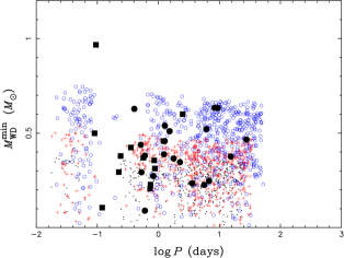
Figure 1: Minimum white-dwarf mass, $M_{\rm WD}^{\rm min}$, versus orbital period, $P$, for sdB stars in short-period binaries (filled symbols; Maxted et al. 2001; Morales-Rueda et al. 2002a,b) and the simulated distribution of sdB stars produced from the 2nd CE ejection channel. Filled squares indicate observed sdB stars with known WD companions, filled circles sdB binaries where the nature of the companion is unknown. The symbols for the simulated systems indicate the actual masses of the white dwarfs (dots: $0.25\leq M_{\rm WD}\leq 0.35\,M_{\odot}$, pluses: $0.35<M_{\rm WD}\leq 0.45\,M_{\odot}$, circles: $0.55\leq M_{\rm WD}\leq 0.65\,M_{\odot}$). The simulation shown uses a standard set of BPS assumptions and CE parameters $\alpha_{\rm CE}=0.75$ and $\alpha_{\rm th}=0.75$ (i.e. similar to our best model parameters; see section 7.4).

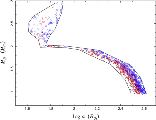
Figure 2: The distribution of the progenitors of sdB binaries (before the 2nd CE phase) in the $a$–$M_{2}$ plane that produces the distribution in Figure 1, where $a$ is the orbital separation and $M_{2}$ is the initial mass of the sdB star on the main sequence. The symbols indicate the mass of the white dwarfs (as in Fig. 1). Solid curves mark the boundaries that produces sdB stars.

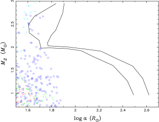
Figure 3: The distribution of Pop I WD binaries in the $a$–$M_{2}$ plane after CE ejection where the first mass-transfer phase is dynamically unstable (with $\alpha_{\rm CE}=0.75$ and $\alpha_{\rm th}=0.75$). The symbols indicate the masses of the white dwarfs (dots: $0.25\leq M_{\rm WD}\leq 0.35\,M_{\odot}$, pluses: $0.35<M_{\rm WD}\leq 0.45\,M_{\odot}$, crosses: $0.45<M_{\rm WD}\leq 0.55\,M_{\odot}$, circles: $0.55<M_{\rm WD}\leq 0.65\,M_{\odot}$, triangles: $M_{\rm WD}>0.65\,M_{\odot}$).

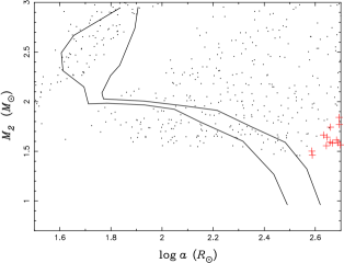
Figure 4: The distribution of Pop I WD binaries in the $a$–$M_{2}$ plane, similar to Figure 3, but where the first mass-transfer is stable leading to conservative RLOF.

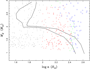
Figure 5: Similar to Figure 3, where the first mass-transfer phase is stable but non-conservative with $\alpha_{\rm RLOF}=0.5$. The mass lost from the system is assumed to take away the same specific angular momentum as pertains to the system (i.e. $\alpha=1.0$ in PJH’s formalism).

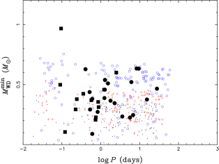
Figure 6: Similar to Figure 1, but for sdB stars with $Z=0.004$.

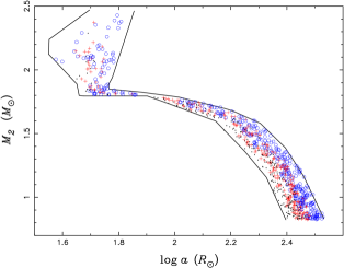
Figure 7: The distribution of the progenitors of sdB binaries (before the 2nd CE phase) in the $a$–$M_{2}$ plane that produces the distribution in Figure 6 (similar to Fig. 2). The symbols indicate the mass of the white dwarfs (dots: $0.25\leq M_{\rm WD}\leq 0.35\,M_{\odot}$, pluses: $0.35<M_{\rm WD}\leq 0.45\,M_{\odot}$, circles: $0.55\leq M_{\rm WD}\leq 0.65\,M_{\odot}$). Solid curves mark the boundaries that produces sdB stars.

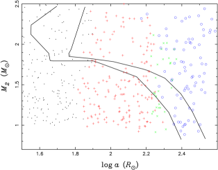
Figure 8: The distribution of WD binaries in the $a$–$M_{2}$ plane for systems where the first mass-transfer phase is stable but non-conservative (with $\alpha_{\rm RLOF}=0.5$; similar to Figure 5 but with $Z=0.004$). The symbols indicate the mass of the white dwarf (as in Fig. 7).

We use the observations of Maxted et al. (2001) and Morales-Rueda et al. (2002a,b) as our main data set to constrain the BPS model. Observationally, two parameters of sdB binaries can be measured accurately, the orbital period $P$ and the mass function $f$ which just depends on the radial velocity amplitude. The latter can be related to a minimum mass of the companion $M^{\rm min}_{\rm comp}$ by choosing an inclination of $\sin i=1$ and adopting a typical mass for the sdB star ($0.5\,M_{\odot}$ in the following). Since the minimum companion mass is more closely related to the physical parameters of the system, we follow common convention and plot the distribution of both the observational data as well as our theoretical distributions in a $M^{\rm min}_{\rm comp}$–$P$ diagram. In Figure 1 the filled symbols show the distribution of the systems in the sample of Maxted et al. (2001) and Morales-Rueda et al. (2002a,b), where we excluded systems with known MS companions.

Since the majority of the sdB stars with known companions have WD companions and since the orbital periods are less than 10 d, this immediately suggests that the majority of sdB binaries in this sample formed through the second CE ejection channel (the second stable RLOF would only produce sdB binaries with long orbital periods, $\sim 1000\,$d). Note that the first CE ejection channel also contributes to the observational data set (in this case, the companion is a main-sequence star instead of a white dwarf).

To illustrate how we can use this diagram as a diagnostic, we have constructed a theoretical distribution of systems assuming that all sdB binaries in our sample originate from the second CE ejection channel. For this purpose we use a simplified BPS model where we adopt simple distributions for the systems before the second CE phase. Specifically we assume here that the WD masses are uniformly distributed between 0.25 and $0.45\,M_{\odot}$ and between 0.55 and $0.65\,M_{\odot}$, that the mass of the sdB star progenitor on the main sequence follows the IMF of Miller & Scalo [1979], and that the logarithm of the separation, $\log(a/R_{\odot})$, is uniformly distributed between 1 and 4. We then determine the post-CE parameters of the systems using our BPS code for chosen CE ejection parameters $\alpha_{\rm CE}$ and $\alpha_{\rm th}$. We further assume that the normal directions of the orbital planes of the sdB stars are randomly distributed and take the mass of the sdB star to be $0.5\,M_{\odot}$, no matter what the actual mass in the simulation is, in order to get $M_{\rm WD}^{\rm min}$ which can then be compared directly to the observational data set.

In Figure 1 we plot the distribution of sdB stars resulting from this simulation, where the symbols indicate the WD masses in the simulation (dots: $0.25\leq M_{\rm WD}\leq 0.35\,M_{\odot}$, pluses: $0.35<M_{\rm WD}\leq 0.45\,M_{\odot}$, circles: $0.55\leq M_{\rm WD}\leq 0.65\,M_{\odot}$). It is apparent that this simulation maps out the observed range of the distribution reasonably well except for KPD 1930+2752, which has a WD mass of $0.97\,M_{\odot}$ (i.e. is more massive than the white dwarfs in this simulation). In this particular simulation, the common-envelope ejection efficiency $\alpha_{\rm CE}$ and the thermal contribution to the CE ejection $\alpha_{\rm th}$ were taken to be 0.75 (as in our best-fit model obtained in § 7.4). We have also tested lower and higher values for $\alpha_{\rm CE}$ and $\alpha_{\rm th}$. As one may imagine, higher values extend the distribution further at long orbital periods and lower values limit the distribution towards shorter orbital periods.

There is a small gap in the left part of the distribution. Subdwarf B stars to the right of the gap are produced from systems where the ZAMS mass of the progenitor is below the helium flash mass (i.e. the first sub-channel), while sdB stars to the left had more massive ZAMS progenitors (see § 3.3). The helium flash mass for Pop I is $M_{0}=1.99\,M_{\odot}$. To allow a better interpolation in this mass range, our model grid includes models with masses very close to the helium flash mass with $M_{\rm ZAMS}=1.90\,M_{\odot}$ and $M_{\rm ZAMS}=2.05\,M_{\odot}$, respectively. If the masses of the two sets were infinitesimally close to the helium flash mass, the gap would disappear. However, this region would still be less densely populated than neighbouring regions.

In order to understand the evolutionary history of these systems better it is more instructive to look at the distribution of the orbital separation $a$ and the mass of the progenitor of the sdB star, $M_{2}$, for systems that become sdB binaries before the CE phase. Figure 2 shows this distribution for the systems shown in Figure 1, where the solid curves mark the boundary of the parameters space that leads to the formation of short-period sdB binaries. Identifying their evolutionary past then becomes a question of what previous evolutionary paths will fill this particular region of parameter space. This depends particularly on whether the first mass-transfer phase, which leads to the formation of the white dwarf, is dynamically stable or unstable.

In Figures 3 and 4 we plot the distributions of WD binaries after the first RLOF phase where the first mass-transfer phase was unstable and stable, respectively (these were obtained from BPS simulations with our standard set of assumptions; see § 4.2).

From Figure 3 it becomes immediately clear that systems where the first mass-transfer phase is dynamically unstable and leads to a CE phase are not likely to be responsible for the production of WD binaries with the required parameters. For the case $\alpha_{\rm CE}=0.75$ and $\alpha_{\rm th}=0.75$ (see case shown), only a few WD binaries populate the marked region in the $a$–$M_{2}$ parameter plane. We have tested that for values $\alpha_{\rm CE}=0.70$ and $\alpha_{\rm th}=0.70$, no systems would satisfy this constraint. Even in the most extreme case with $\alpha_{\rm CE}=1.0$ and $\alpha_{\rm th}=1.0$, the maximum values physically allowed, the right part of the marked region (with $\log a>2.2$) which is in fact the most important part, cannot be populated. We can therefore safely conclude that the first RLOF phase for the progenitors of short-period sdB stars is likely to have been stable.

In Figure 4 we plot the WD binaries that result from a first stable RLOF phase assuming that mass transfer is conservative (i.e. $\alpha_{\rm RLOF}=1$) and where we use $q_{\rm crit}=1.2$ in the stability criterion (consistent with the results from Paper I). The region of interest is now populated by two distinct groups of systems separated by a gap. The WD binaries in the upper-left corner are systems that experienced stable RLOF in the Hertzsprung gap while systems below the gap fill their Roche lobe first on the FGB. This evolutionary path tends to produce low-mass white dwarfs ($\la 0.35\,M_{\odot}$, indicated as dots), so this cannot explain the many more massive WDs in Figure 1. This implies that the first RLOF phase cannot be conservative, at least not as a rule.

In Figure 5 we show a similar distribution, but now assuming that the first RLOF is non-conservative with $\alpha_{\rm RLOF}=0.5$ and that the mass lost takes away the same specific angular momentum as pertains to the system ($\alpha=1$ in the PJH formalism). The distribution fills the parameter space of interest reasonably well, and the WD masses are also widely distributed as required. We generally find that using lower values of $\alpha_{\rm RLOF}$, reduces the mass $M_{2}$ and shortens the orbital period. If $\alpha_{\rm RLOF}$ is too small (i.e. mass transfer is very non-conservative), the most important part of the parameter space, the lower-right part with $\log a>2$, cannot be filled. Increasing the value of $\alpha$ increases the angular-momentum loss per unit mass lost from the system. Hence higher values of $\alpha$ produce shorter orbital periods. Again the lower-right part cannot be filled for values of $\alpha=1.5$ and larger. For $\alpha=0.5$, all the parts of the space are filled, but only with relatively low-mass WDs ($\la 0.45\,M_{\odot}$). We also tested some cases where the mass lost takes away the same specific angular momentum as pertains to the mass donor or the mass gainer (for $\alpha_{\rm RLOF}=0.75$, 0.50 and 0.25, respectively). In these cases, all parts of the parameter space are filled, but only with low-mass white dwarfs ($<0.45\,M_{\odot}$).

The main conclusion of these comparisons is that, in order to obtain a wide coverage of the parameter space that can lead to the formation of short-period sdB binaries, the first phase of mass transfer has to be non-conservative, where our best-choice parameters are $\alpha_{\rm RLOF}=0.5$ and $\alpha\simeq 1.0$.

All of these results are, however, dependent on the metallicity of the population. To examine this, we carried out a similar set of tests for a typical thick-disc metallicity of $Z=0.004$. The results of these simulations are shown in Figures 6 to 8. The results are broadly similar, except that there is a systematic shift in the distribution towards shorter separations and lower masses $M_{2}$ (most clearly seen when comparing Figs. 5 and 8).

Finally we note that, if we had used the criterion for stable RLOF based on a polytropic model [1987, 1988, 1997, 2001], revised to take into account non-conservative mass transfer, we would have obtained a very small number of WD binaries, but none of them would actually populate the required parameter space for $\alpha_{\rm RLOF}=0.5$ and $\alpha=1.0$.

6 Monte Carlo simulations

Table 1: Birthrates of sdB stars from different channels (in $10^{-3}\,{\rm yr}^{-1}$)

set	$Z$	$n(1/q)$	$q_{\rm crit}$	$\alpha_{\rm CE}$	$\alpha_{\rm th}$	1st CE	1st RLOF	2nd CE	2nd RLOF	sdB Binary	Merger	Total
1	0.02	a	1.5	0.5	0.5	5.51	29.89	2.80	0.00	38.20	17.22	55.42
2	0.02	a	1.5	0.75	0.75	6.80	29.89	5.44	0.00	42.13	16.62	58.75
3	0.02	a	1.5	1.0	1.0	8.41	29.89	8.38	0.00	46.68	16.24	62.93
4	0.02	b	1.5	0.5	0.5	7.22	3.46	0.32	0.00	11.00	3.30	14.31
5	0.02	b	1.5	0.75	0.75	9.16	3.46	0.55	0.00	13.17	3.22	16.39
6	0.02	b	1.5	1.0	1.0	11.23	3.46	0.79	0.00	15.48	3.06	18.54
7	0.02	a	1.2	0.5	0.5	7.02	22.25	1.58	0.00	30.84	8.51	39.36
8	0.02	a	1.2	0.75	0.75	8.62	22.25	2.98	0.00	33.85	8.25	42.09
9	0.02	a	1.2	1.0	1.0	10.71	22.25	5.43	0.00	38.38	7.99	46.38
10	0.004	a	1.2	0.5	0.5	8.21	26.22	2.00	0.00	36.43	10.28	46.71
11	0.004	a	1.2	0.75	0.75	10.56	26.22	3.82	0.00	40.60	9.95	50.55
12	0.004	a	1.2	1.0	1.0	13.19	26.22	5.79	0.00	45.20	9.38	54.58

Table 2: Percentages of sdB stars from different channels and the total numbers (in $10^{6}$) in the Galaxy at the current epoch

set	$Z$	$n(1/q)$	$q_{\rm crit}$	$\alpha_{\rm CE}$	$\alpha_{\rm th}$	1st CE	1st RLOF	2nd CE	2nd RLOF	sdB Binary	Merger	Total Number
												($10^{6}$)
1	0.02	a	1.5	0.5	0.5	14.63	61.75	4.88	0.00	81.25	18.75	7.04
						28.09	0.00	14.85	0.00	42.94	57.06	2.31
						53.72	0.00	22.37	0.00	76.09	23.91	1.08
2	0.02	a	1.5	0.75	0.75	17.92	55.05	5.08	0.00	78.05	21.95	7.92
						27.93	0.00	13.55	0.00	41.49	58.51	2.97
						39.35	0.00	15.65	0.00	55.00	45.00	1.63
3	0.02	a	1.5	1.0	1.0	19.74	45.56	10.63	0.00	75.94	24.06	9.52
						24.26	0.00	23.21	0.00	47.47	52.53	4.36
						27.51	0.00	17.24	0.00	44.75	55.25	2.45
4	0.02	b	1.5	0.5	0.5	61.32	25.46	2.30	0.00	89.08	10.92	2.41
						80.68	0.00	3.36	0.00	84.04	15.96	1.65
						92.96	0.00	2.95	0.00	95.91	4.09	1.24
5	0.02	b	1.5	0.75	0.75	67.23	19.42	1.93	0.00	88.59	11.41	3.15
						81.72	0.00	2.65	0.00	84.37	15.63	2.30
						87.96	0.00	2.56	0.00	90.52	9.48	1.58
6	0.02	b	1.5	1.0	1.0	70.34	15.37	3.32	0.00	89.04	10.96	4.07
						81.45	0.00	4.32	0.00	85.76	14.24	3.14
						81.77	0.00	2.98	0.00	84.75	15.25	1.76
7	0.02	a	1.2	0.5	0.5	30.82	46.19	5.49	0.00	82.51	17.49	4.12
						40.26	0.00	14.28	0.00	54.54	45.46	1.58
						63.83	0.00	20.24	0.00	84.07	15.93	0.87
8	0.02	a	1.2	0.75	0.75	36.37	39.44	5.17	0.00	80.98	19.02	4.80
						41.18	0.00	12.57	0.00	53.76	46.24	1.97
						52.50	0.00	14.40	0.00	66.90	33.10	1.18
9	0.02	a	1.2	1.0	1.0	37.73	31.31	11.68	0.00	80.72	19.28	6.04
						35.93	0.00	24.18	0.00	60.11	39.89	2.92
						39.97	0.00	16.92	0.00	56.89	43.11	1.63
10	0.004	a	1.2	0.5	0.5	31.51	44.40	6.16	0.00	82.07	17.93	4.33
						37.10	0.00	16.08	0.00	53.17	46.83	1.66
						59.05	0.00	23.59	0.00	82.64	17.36	0.95
11	0.004	a	1.2	0.75	0.75	36.33	36.57	6.22	0.00	79.12	20.88	5.16
						34.95	0.00	14.93	0.00	49.88	50.12	2.15
						46.55	0.00	16.93	0.00	63.47	36.53	1.34
12	0.004	a	1.2	1.0	1.0	38.35	28.56	12.70	0.00	79.62	20.38	6.66
						31.44	0.00	26.32	0.00	57.76	42.24	3.22
						36.96	0.00	17.03	0.00	53.99	46.01	1.82

In order to investigate the formation of sdB stars from the various channels more systematically, we performed 12 sets of Monte Carlo simulations altogether for a Pop I and a thick-disc population ($Z=0.004$) by varying the model parameters over a reasonable range. Specifically, we varied the parameter $\alpha_{\rm CE}$ for the CE ejection efficiency and the parameter $\alpha_{\rm th}$ for the thermal contribution to CE ejection from 0.5 to 1.0, the value of $q_{\rm crit}$ in the criterion for a first phase of stable RLOF on the FGB or AGB from 1.2 to 1.5. Two initial mass-ratio distributions were adopted: a constant mass-ratio distribution and one where the masses are uncorrelated and drawn independently from a Miller-Scalo IMF. Guided by the results from the previous section, we assume in all of these simulations that the first stable RLOF phase is non-conservative (with $\alpha_{\rm RLOF}=0.5$) and that the mass lost takes away the same specific angular momentum as pertains to the system. We assume that one binary with its primary more massive than $0.8\,M_{\odot}$ is formed annually in the Galaxy for both the Pop I and the thick-disc population. Note that this star-formation rate is almost certainly too high for the thick-disc population and that therefore these results should be scaled down accordingly.

Table 1 lists the birthrates of sdB stars produced from the various formation channels. In the table, the 2nd column denotes the metallicity ($Z=0.02$ for Pop I and $Z=0.004$ for the thick-disc population); the 3rd column indicates the initial mass-ratio distribution, where ‘a’ represents a constant mass-ratio distribution and ‘b’ one of uncorrelated component masses; the 4th column gives $q_{\rm crit}$, the critical mass ratio for the first stable RLOF on the FGB or AGB; the 5th and the 6th columns give the values of $\alpha_{\rm CE}$ and $\alpha_{\rm th}$ adopted, respectively. Galactic birthrates for sdB stars (in $10^{-3}\,{\rm yr}^{-1}$) from the first CE ejection channel, the first stable RLOF channel, the second CE ejection channel and the second stable RLOF channel are listed in columns 7 to 10. The 3rd column from the right gives the birthrates of sdB binaries, and the 2nd column from the right gives the birthrates of single sdB stars resulting from the helium WD merger channel. The last column gives the total birthrates of sdB stars from all channels.

Table 2 lists the percentages of sdB stars from various channels and the total numbers in the Galaxy at the current epoch. Columns 1 - 6 list the main model parameters as in Table 1. Percentages of sdB stars from the first CE ejection channel, the first stable RLOF channel, the second CE ejection channel and the second stable RLOF channel are given in columns 7 to 10. The 3rd column from the right gives the percentages of sdB binaries, and the 2nd column from the right the percentages of single sdB stars resulting from the helium WD merger channel. The last column gives the total numbers (in $10^{6}$) of sdB stars from all the channels in the Galaxy.

For each item in the table we list three numbers. The first row gives the number for sdB stars without taking any observational selection effects into account and therefore represents the intrinsic distribution, the second row takes into account the GK selection effect, i.e. excludes any sdB binaries where the secondary is of spectral type K or earlier, and the third row takes into account the GK and the strip selection effects as to best represent the sample of Maxted et al. (2001).

Various model parameters from these simulations are plotted in Figures 9 to  27, which will be discussed in detail in the next section.

7 Discussion

As summarized in § 3, we altogether consider five channels for the formation of sdB stars: the first CE ejection channel, the first stable RLOF channel, the second CE ejection channel, the second stable RLOF channel and the double He WD merger channel. The birthrates of sdB stars formed from each channel and the relative percentages at the current epoch are listed in Tables 1 and  2, respectively.

As these tables show, the relative importance of the five channel varies significantly for the different sets of parameters. The first CE ejection, the first stable RLOF and the merger channels are the most important ones intrinsically. However, once selection effects are taken into account, the second CE ejection channel becomes of comparable importance. As mentioned before, for our set of assumptions we do not obtain sdB stars from the second stable RLOF channel. Note also that the GK selection effect tends to remove all of the sdB binaries from the first stable RLOF channel.

7.1 Sensitivity to the model parameters

Our BPS model requires a number of model parameters and input distributions. The parameters/distributions which we varied in the study are: $q_{\rm crit}$, the critical mass ratio above which mass transfer is dynamically unstable on the FGB/AGB, the mass-transfer efficiency $\alpha_{\rm RLOF}$, which defines the fraction of mass lost from the primary that is accreted by the gainer for systems experiencing stable RLOF after the main-sequence phase, the specific angular momentum $\alpha$ lost from the system/unit mass during stable RLOF, the CE ejection efficiency $\alpha_{\rm CE}$ and the thermal contribution factor $\alpha_{\rm th}$ in the CE ejection criterion, the initial mass-ratio distribution $n(1/q)$ and the metallicity of the population.

As was shown in § 5, $q_{\rm crit}$, $\alpha_{\rm RLOF}$ and $\alpha$ are strongly constrained by the $\log P$ - $M_{\rm WD}^{\rm min}$ diagram of the observations by Maxted et al. (2001) and Morales-Rueda et al. (2002a,b). In order to match the observed distribution, the value for $q_{\rm crit}$ cannot be taken from a simple polytropic model [1987, 1988, 1997], even in a revised version taking non-conservative RLOF into account [2001], as such a $q_{\rm crit}$ would make a first phase of stable RLOF very unlikely and would not produce WD binaries with the parameters required to explain the sample of Maxted et al. (2001). Completely conservative RLOF ($\alpha_{\rm RLOF}=1$) or the assumption that the mass lost from the system takes away the same specific angular momentum as pertains to the primary/secondary also cannot explain the observations. This analysis favours values $\alpha_{\rm RLOF}\simeq 0.5$ and $\alpha\simeq 1$ (in units of ${2\pi a^{2}/P}$); we adopted these value for all of our simulations.

We investigated two values for $q_{\rm crit}$, 1.2 and 1.5. The higher value implies that the mass donor can be more massive and that the first stable RLOF phase then results in WD binaries with more massive WD companions (see Figures 13 and  14). Obviously, a higher $q_{\rm crit}$ leads to fewer sdB stars from the first CE ejection channel, more from the first stable RLOF channel and more from the second CE ejection channel. As a consequence, the birthrate of sdB binaries is increased significantly (see Table 1); however, the fraction of sdB binaries is not influenced significantly, as the merger rate also increases.

An increase in $\alpha_{\rm CE}$ and $\alpha_{\rm th}$ makes it easier to eject the CE and hence leads to a systematic increase in the post-CE orbital periods of sdB binaries from the first CE ejection and the second CE ejection; it also leads to higher birthrates from these two channels, but decreases the rate from the merger channel (since fewer systems will merge in the age of the Galaxy). However, the binary fraction of sdB stars at the current epoch decreases. The reason is that the envelope of a star near the tip of the FGB for ZAMS masses less than the helium flash mass $M_{0}$ is loosely bound and can be easily ejected for a wide range of these parameters. Therefore the main effect of an increase in $\alpha_{\rm CE}$ and $\alpha_{\rm th}$ is to increase the numbers of CE ejections for stars with ZAMS masses greater than $M_{0}$. As their envelopes are tightly bound and the sdB binaries formed this way have very short orbital periods, they merge soon after their formation. On the other hand, the increase of $\alpha_{\rm CE}$ and $\alpha_{\rm th}$ makes helium WD pairs with a low total mass more likely, and therefore the sdB stars from the merger channel generally have a lower mass. Since the timescale for helium burning for a low-mass sdB star is significantly longer in this case, this leads to an increased contribution of sdB stars formed through the merger channel at the current epoch.

As compared to the constant initial mass-ratio distribution, the distribution for uncorrelated component masses means that a star is more likely to have a low-mass companion. Therefore this distribution leads to more sdB stars from the first CE ejection channel and greatly decreases the numbers of sdB stars from the first stable RLOF, the second CE ejection and the merger channel. The overall result is that the binary fraction of sdB stars increases significantly by about 10 per cent.

The evolutionary timescale for stars of a given mass is shorter for stars with a thick-disc metallicity $Z=0.004$ than the corresponding timescale for Pop I objects. This implies that stars of lower mass can evolve to become sdB star within the age of the Galaxy. Since these lower-mass stars are relatively more common, the numbers of sdB stars of a thick-disc population from all the channels would be larger than that of Pop I for the same star-formation rate. The binary fraction of sdB stars at the current epoch is somewhat higher than for Pop I. The reason is that sdB binaries from the CE ejection channels are more likely from low-mass FGB stars for a thick-disc population due to their shorter evolutionary timescales, and the orbital periods of those sdB binaries resulting from low-mass FGB stars are so long that they will not merge in the lifetime of the Galaxy. A higher WD mass is also more likely for sdB binaries for the thick-disc population from the second CE ejection channel (see Fig. 14), as the core mass of a FGB/AGB star is more likely to be massive and therefore the WD binary resulting from the first RLOF is more likely to contain a massive WD.

7.2 The distribution of orbital periods

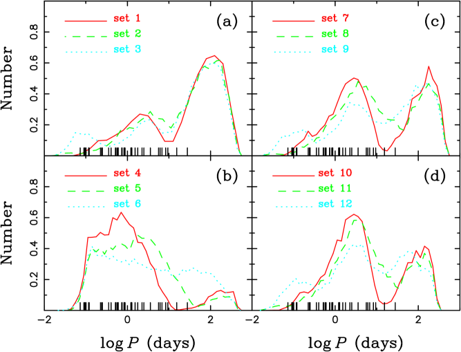
Figure 9: The distribution of orbital periods of sdB stars from all the simulation sets. The short ticks along the X-axis indicate the positions of sdB stars in the observational sample (Maxted et al. 2001; Morales-Rueda et al. 2002a,b). Panels (a) and (b) illustrate how the results depend on the initial mass ratio distribution with panel (a) using a flat distribution and panel (b) a distribution with uncorrelated component masses. Panels (a) (with $q_{\rm crit}=1.5$) and (c) (with $q_{\rm crit}=1.2$) show the effect of changing the critical mass ratio for stable RLOF on the FGB/AGB. Panels (c) and (d) demonstrate the metallicity dependence (with $Z=0.02$ and 0.004, respectively).

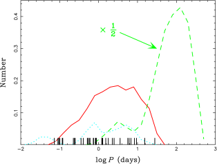
Figure 10: The distribution of orbital periods of sdB stars from different channels in simulation set 2 (with $Z=0.02$, a flat mass ratio distribution, $q_{\rm crit}=1.5$, $\alpha_{\rm CE}=\alpha_{\rm th}=0.75$) (solid: the first CE ejection channel, dashed: the first stable RLOF channel, dotted: the second CE ejection channel). No sdB stars are produced from the second stable RLOF channel. The curve for the first stable RLOF channel has been rescaled by a factor of 1/2 for clarity. Short ticks along the X-axis indicate the positions of sdB stars in the observational sample (Maxted et al. 2001; Morales-Rueda et al. 2002a,b.

Figure 9 shows the distribution of orbital periods of sdB binaries at the current epoch for simulation sets 1 to 12. The orbital period ranges from 0.5 hr to 500 d (see also Figure 10). While the lower limit is essentially fixed by the condition that neither component fills its Roche lobe and therefore mainly depends on the radii of both components, the upper limit is mainly determined by how much angular momentum is lost during the first stable RLOF phase. Some of the distributions, such as those in simulation sets 3, 9 and 12 with high CE ejection efficiency, have three peaks. The leftmost peak comes from the second CE ejection channel where the donor’s ZAMS mass is greater than the helium flash mass $M_{0}$. In this case, the envelope is tightly bound and the WD has to penetrate very deep before the envelope can be ejected, which leads to a very short orbital period of the sdB binary. The central peak contains systems from the first and the second CE ejection channels where the donor’s ZAMS mass is less than $M_{0}$. The envelope is more loosely bound in this case, leading to a longer post-CE orbital period. The rightmost peak is due to sdB binaries from the first stable RLOF channel, which always produces systems with long orbital periods.

Panel (b) shows that sdB binaries from the first CE ejection channel dominate for the simulations where the initial component masses are uncorrelated. Note that in this case very few sdB binaries are formed in the first RLOF channel since for uncorrelated masses the first mass-transfer phase is dynamically unstable in most cases.

In Figure 10 we present the distribution of orbital periods of sdB binaries at the current epoch from the different channels of simulation set 2 (with $Z=0.02$, a flat mass ratio distribution, $q_{\rm crit}=1.5$, $\alpha_{\rm CE}=\alpha_{\rm th}=0.75$). sdB stars from the first CE ejection channel have orbital periods from 1.5 hr to 40 d, where the lower limit is again constrained by the radii of the MS companions and the upper limit depends strongly on the CE ejection efficiency $\alpha_{\rm CE}$ and the thermal contribution $\alpha_{\rm th}$ to the CE ejection. In the extreme case ($\alpha_{\rm CE}=\alpha_{\rm th}=1$), the upper limit can be as high as 400 d. sdB stars from the first stable RLOF channel have orbital periods from 15 hr to 500 d, and the orbital-period range is sensitive to the assumption concerning the systemic angular momentum loss during the first stable RLOF phase. The distribution has two peaks. The left peak is caused by sdB stars that experience stable RLOF in the Hertzsprung gap where the donor’s ZAMS mass is larger than $M_{0}$, while the right peak is dominated by systems undergoing stable RLOF on the FGB. (Note that the minimum mass of the helium remnant which will ignite helium in the core is $\sim 0.33\,M_{\odot}$ for stars with a ZAMS mass greater than $M_{0}$; this value depends, however, on the initial mass ratio; see Han, Tout & Eggleton 2000 for details.) The left peak is much smaller than the right peak since all the donors in this group have to be quite massive and hence for the adopted IMF have a lower probability. In addition, their companions are likely to be massive as well in this simulation with a constant mass-ratio distribution and have a relatively short evolution time. For example, the lifetime of a Pop I star with a ZAMS mass of $2.5\,M_{\odot}$ on the main sequence is $\sim 7.7\times 10^{8}\,{\rm yr}$ and the lifetime of a $3.2\,M_{\odot}$ star is $\sim 4.0\times 10^{8}\,{\rm yr}$. Such lifetimes are comparable to the core-helium burning lifetime of low-mass sdB stars: e.g. the core-helium burning lifetime of a $0.35\,M_{\odot}$ sdB star is $\sim 6.2\times 10^{8}\,{\rm yr}$. This has the consequence that the companion star will fill its Roche lobe while the sdB star is still burning helium in the core and the system may then no longer have the appearance of a sdB binary (i.e. be a helium-burning star with a thin hydrogen-rich envelope). On the other hand, a donor experiencing stable RLOF on the FGB is likely to be less massive and both components will have longer evolutionary timescales and mass transfer will not occur while the sdB star is still in the helium core-burning phase.

The second CE ejection channel produces sdB binaries with orbital periods from 0.5 hr to 25 d. The distribution has two parts, separated by a well-defined gap. The left part contains systems where the donor’s ZAMS mass is greater than $M_{0}$, and the right part systems with ZAMS donor masses less than $M_{0}$. The gap is caused by the sharp drop of the radius at the tip of the FGB from stars with ZAMS masses somewhat smaller than $M_{0}$ relative to stars with ZAMS masses somewhat greater than $M_{0}$ (see Fig. 8 and Table 1 of Paper I). This sharp drop leads to a great decrease in the radius range for which a star can fill its Roche lobe, eject the common envelope and is then able to ignite helium in the core. The right part has two peaks, caused by the bimodal distribution of the masses of the WD companions. Note that the sdB stars from the first CE ejection channel fill in the gap because of the large range of masses for the MS companions. In contrast, sdB stars from the second CE ejection channel all have WD companions whose masses are restricted to a rather narrow range. The second stable RLOF channel does not produce any sdB stars in this model since mass-transfer is dynamically unstable in all cases. To obtain systems from this channel requires a tidally enhanced stellar wind. As shown in Paper I, sdB binaries produced from the second stable RLOF phase would have orbital periods in the range of 400 to 1500 d.

7.3 The distribution of masses

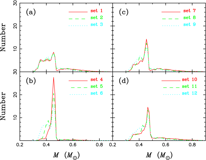
Figure 11: Distribution of masses of sdB stars from all the simulation sets. Panels (a) and (b) show the effect of a change in the initial mass ratio distribution with panel (a) using a flat distribution and panel (b) a distribution of uncorrelated component masses. The effect of a change in the critical mass ratio for stable RLOF on the FGB/AGB is shown in panels (a) ($q_{\rm crit}=1.5$) and (c) ($q_{\rm crit}=1.2$). Panels (c) and (d) are for different metallicities ($Z=0.02$ and 0.004, respectively).

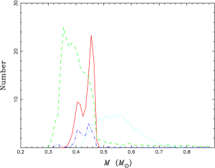
Figure 12: Distribution of masses of sdB stars from different channels in simulation set 2 (with $Z=0.02$, a flat mass ratio distribution, $q_{\rm crit}=1.5$, $\alpha_{\rm CE}=\alpha_{\rm th}=0.75$) (solid: the first CE ejection channel, dashed: the first stable RLOF channel, dot-dashed: the second CE ejection channel, dotted: the merger channel). No sdB stars are produced from the second stable RLOF in this simulation.

Figure 11 displays the distributions of the masses of sdB stars from all the simulation sets. The overall mass range is quite wide, ranging from $\sim 0.3\,M_{\odot}$ to $\sim 0.8\,M_{\odot}$. The distribution does not depend much on the CE ejection efficiency ($\alpha_{\rm CE}$) or the thermal contribution to CE ejection ($\alpha_{\rm th}$). The distribution is mainly determined by $q_{\rm crit}$, the critical mass ratio for stable RLOF on the FGB or the AGB, and the initial mass-ratio distribution. As a matter of fact, the distribution is mainly controlled by the contribution of systems from the first stable RLOF channel. When this contribution is large, as in simulation sets 1, 2 and 3 ($q_{\rm crit}=1.5$ and with a flat initial mass ratio distribution), the distribution is wide and flat (0.35 - $0.47\,M_{\odot}$ in panel a). If the contribution is insignificant, as in simulation sets 4, 5 and 6 ($q_{\rm crit}=1.5$ and with an initial mass ratio distribution of uncorrelated component masses), the distribution is narrow and sharply peaked (the peak at $0.46\,M_{\odot}$ in panel b).

Figure 12 gives the distributions from different channels in simulation set 2 (with $Z=0.02$, a flat mass ratio distribution, $q_{\rm crit}=1.5$, $\alpha_{\rm CE}=\alpha_{\rm th}=0.75$). The distribution for the 1st CE ejection channel has a sharp major peak at $0.46\,M_{\odot}$ and a secondary peak at $0.4\,M_{\odot}$. The secondary peak is due to the fact that the stellar radius range for CE ejection near the tip of the FGB to produce sdB stars is wider for $M_{\rm ZAMS}=1.90$ than for $M_{\rm ZAMS}\leq 1.60\,M_{\odot}$ (see Table 1 in Paper I); as a consequence, CE ejection for stars around $M_{\rm ZAMS}=1.90$ results in relatively low-mass sdB stars which have relatively long helium-burning lifetimes.

The first stable RLOF channel produces a plateau (or broad peak) in the distribution at low masses, and the distribution drops sharply near $0.47\,M_{\odot}$, as most systems experiencing stable RLOF in the Hertzsprung gap result in low-mass sdB stars, while the maximum mass is limited by the core mass at the tip of the FGB at which the helium flash or helium ignition occurs.

The distribution for the 2nd CE ejection channel has three peaks, the small left one at $0.33\,M_{\odot}$ represents systems with a ZAMS donor mass greater than the helium flash mass. The central one and the right one are analogous to the two peaks in the first CE ejection channel. Finally, the merger channel produces a relatively wide and flat distribution from 0.42 to $0.72\,M_{\odot}$.

7.4 The best-choice model

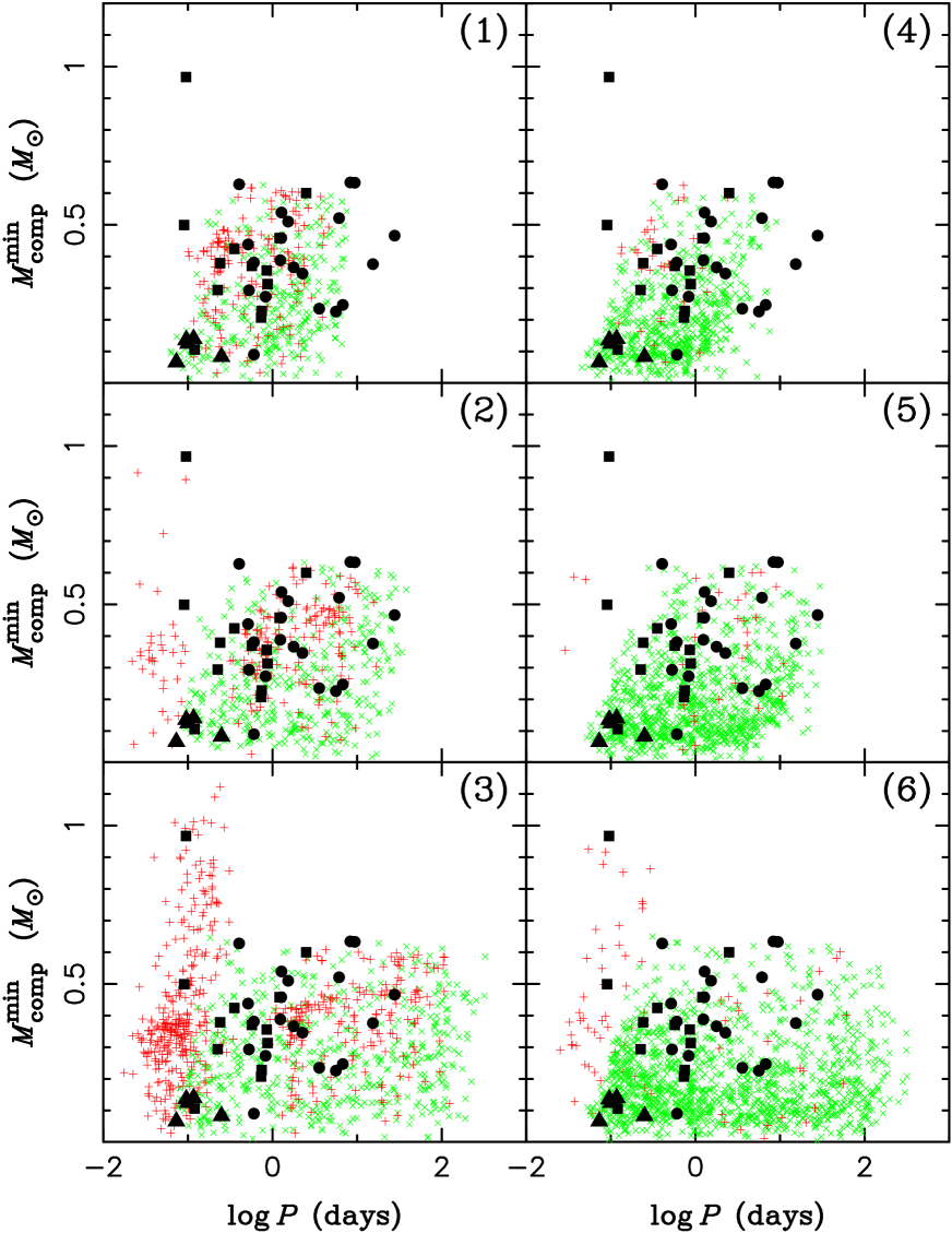
Figure 13: The distribution of sdB stars at the current epoch from simulations 1 to 6 (as indicated in the upper-right corner of each panel) in a $\log P$ - $M_{\rm comp}^{\rm min}$ diagram, where $P$ is the orbital period and $M_{\rm comp}^{\rm min}$ the minimum companion mass as defined in the observations of Maxted et al. (2001). Filled squares represent observed sdB stars with WD companions, filled triangles observed sdB stars with dM companions and filled circles observed sdB stars with companions of unknown type (see Morales-Rueda et al. 2002b). Pluses indicate sdB stars formed from the 2nd CE ejection channel with WD companions, crosses represent sdB stars from the 1st RLOF phase (either the first CE ejection or the first stable RLOF channel) with MS companions. In all panels, the GK selection is included (i.e. systems with MS companions hotter than $4000$K were excluded).

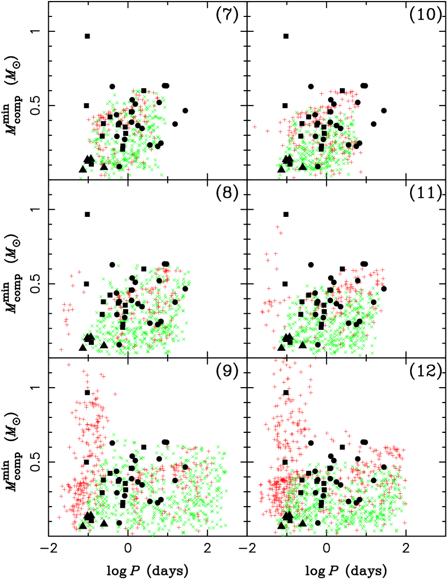
Figure 14: Similar to Figure 13, but for simulations 7 to 12 as indicated in the upper-right corner of each panel.

The orbital periods $P$ and the mass function, or equivalently the minimum component masses $M_{\rm comp}^{\rm min}$ (obtained from the mass function by assuming that the mass of the sdB star is $0.5\,M_{\odot}$ and the inclination $\sin i=1$) can be determined quite precisely from the observational data set of Maxted et al. (2001) and Morales-Rueda et al. (2002a,b). Therefore we choose our best model by mapping the theoretical distribution in the observational $P$ - $M_{\rm comp}^{\rm min}$ diagram. A two-dimensional mapping of this type constrains the BPS model much more severely than any one-dimensional distribution could. We plotted the $P$ - $M_{\rm comp}$ diagram for all of our simulation sets in Figures 13 and  14. For a sdB binary produced from our simulations, we assume that the normal direction of the orbital plane is randomly distributed in all solid angles. We then take $\sin i=1$ and $M_{\rm sdB}=0.5\,M_{\odot}$, no matter what their actually values are, in order to mimic how this diagram is constructed observationally. Here we include the GK selection effect, which is the major selection effect, in the plotting, but do not consider the strip selection effect as some of the observational data points are not affected by it, nor do we include the $K$ selection effect. In Figures 13 and  14, plus symbols represent sdB binaries with WD companions and crosses sdB binaries with MS companions (or red-giant companions) from the simulations. Filled squares represent observed sdB binaries with WD companions, filled triangles observed sdB binaries with MS companions and filled circles observed sdB binaries of unknown companion type. Visual inspection of these distributions shows that several of the simulations are in reasonable agreement with the observational distribution, where simulation set 2 (with $Z=0.02$, a flat mass ratio distribution, $q_{\rm crit}=1.5$, $\alpha_{\rm CE}=\alpha_{\rm th}=0.75$) provides the best overall fit. Based on this comparison, we choose set 2 as our best-fit model.

Even though the overall distribution in set 2 agrees quite well with the observed one, the agreement is by no means perfect. The density of points near the sdB star KPD 1930+2752 (the filled square at the top-left corner of panel 2 in Figure 13) is quite low. This may be due to the fact that KPD 1930+2752 was specially selected as a p-mode pulsating star. It was found by Billéres et al. [2000] in a search for pulsators of the EC 14026 variety [1997] and may therefore not be a very representative system. It is also quite possible, perhaps even likely, that the CE ejection efficiency is not constant for all systems as we assumed. A higher CE ejection efficiency for this system could explain it easily (e.g. see panel 3 of Figure 13).

Simulation set 2 is quite similar to simulation set 8, except that in the latter $q_{\rm crit}=1.2$ instead of $q_{\rm crit}=1.5$. For a higher $q_{\rm crit}$, the mass donor in the first RLOF phase tends to be more massive, and therefore the first stable RLOF phase is more likely to produce WD binaries with high WD masses. The sdB binaries from the second CE ejection channel therefore tend to have more massive WD companions (compare panel 2 of Fig. 13 with panel 8 of Fig. 14). A value of $q_{\rm crit}$ of 1.5 is higher than the critical value for dynamical mass transfer obtained from actual binary evolution calculations (see section 5.1 and Table 3 in Paper I) and may be in indication for tidally enhanced mass transfer (see the discussion in section 4.1). It may also by caused by our rather simple treatment of the first stable RLOF phase on the FGB/AGB. We assume that the final WD mass is equal to the core mass of the donor at the onset of the RLOF phase. However, the core mass increases somewhat during stable RLOF; thus the final WD mass depends on the duration of the mass-transfer phase which in turn is quite sensitive to $\alpha_{\rm RLOF}$ [2002], an effect that needs to be studied further.

7.5 sdB binaries with main-sequence companions

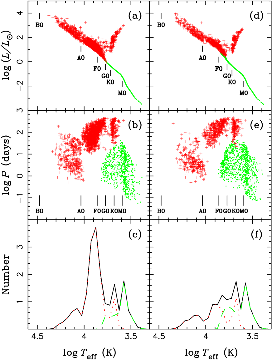
Figure 15: The characteristics of the MS secondaries in sdB binaries from the first CE ejection channel (dots) and the first stable RLOF channel (crosses) for the best-fit simulations 2 (with $q_{\rm crit}=1.5$; left panels) and 8 (with $q_{\rm crit}=1.2$; right panels). Panels (a) and (d): HRD with spectral types indicated along the main sequence (based on Zombeck 1990). Panels (b) and (e): orbital period versus effective temperature. Panels (c) and (f): the distribution of $\log T_{\rm eff}$; solid curves: both channels; dashed curves: the first CE ejection channel only; dotted curves: the first stable RLOF channel.

Our best-fit model is mainly constrained by systems that experienced a CE phase, where in many cases the companion is a white dwarf. Using our best fits (simulations 2 and 8), our BPS model then makes more general predictions about the distribution of the properties of sdB binaries with MS companions. In Figure 15 we present some of the characteristics of the secondaries in these systems: in the HRD (panels a and d), in the $P_{\rm orb}$ – $T_{\rm eff}$ diagram (panels b and e) and the distributions of $T_{\rm eff}$ (panels c and f), where the panels on the left represent simulation 2 (with $q_{\rm crit}=1.5$) and on the right simulation 8 (with $q_{\rm crit}=1.2$). In the upper panels, dots represents systems from the first CE ejection channel and plus symbols from the first stable RLOF channel.

In these panels, one can distinguish four groups of systems, most clearly seen in the middle panels, corresponding to four peaks in the $T_{\rm eff}$ distribution in the bottom panels. The systems formed through the first CE ejection channel (dots) tend to have secondaries of the latest spectral type (F to M) and have the shortest orbital periods. Because the secondaries are significantly less massive than the initial MS mass of the sdB star (due to the $q_{\rm crit}$ constraint), they are essentially unevolved and hence lie close to the ZAMS in the HRD. Indeed most of the secondaries have spectral type M (see the ridge in the central panels and the right peak in the bottom panels). Below an orbital period of $\sim 12\,$hr most and below $\sim 6\,$hr all sdB binaries from the first CE ejection channel have M dwarf companions, consistent with the fact that all of the 5 sdB binaries with known MS companions have M type secondaries (see e.g. Fig. 16). The reason for this is simply that these very low-mass stars have to spiral much deeper into the envelope during the CE phase before enough orbital energy has been released to eject the envelope, leading to shorter post-CE orbital periods. Above a period of $\sim 12\,$hr there is an increasing number of secondaries of earlier spectral type (as early as F), even though the systems with M dwarf companions still dominate (this is more prominent in simulation 2 with $q_{\rm crit}=1.5$ than simulation 8 with $q_{\rm crit}=1.2$).

The two groups of systems with the longest orbital periods, mainly with secondaries of spectral type A to K, are systems from the first stable RLOF where mass transfer started on the FGB. The gap between these two groups is just due to the Hertzsprung gap. The systems with secondaries of the earliest spectral type (mainly A) are also systems from the first stable RLOF channel, but where mass transfer started when the progenitor of the sdB star was in the Hertzsprung gap. Since in our model the critical mass ratio for stable RLOF is much larger for systems in the Hertzsprung gap ($q_{\rm crit}=3.2$) than for stars on the FGB ($q_{\rm crit}=1.2$/1.5), the companions in the former can accrete much more mass in the first stable mass-transfer phase, and hence the secondaries of the sdB stars tend to be more massive and of earlier spectral type. Furthermore because of the larger added mass, they are rejuvenated to a larger degree and therefore are on average somewhat less evolved than secondaries that accreted from a FGB star (causing the kink around spectral type A0, most clearly seen in panel d). We note that the precise distributions of the secondaries in these diagrams are somewhat sensitive to the assumptions concerning the stable mass-transfer phase, in particular $\alpha_{\rm RLOF}$, $\alpha$, $q_{\rm crit}$ and the treatment of the rejuvenation in our simulations. For example, a lower value of $\alpha_{\rm RLOF}$ would systematically move the distributions towards lower temperatures.

The comparison of the panels on the left with those on the right illustrates how dramatically the number of sdB binaries with MS stars depends on $q_{\rm crit}$. For $q_{\rm crit}=1.5$ (left), these completely dominate the overall distribution (see the large peak in panel c), while for $q_{\rm crit}=1.2$ (right) they only form a significant subset. This has the interesting implication that observations of such systems and the determination of their frequency relative to short-period systems could help constrain $q_{\rm crit}$, or more generally the conditions for dynamical mass transfer and/or the importance of tidally enhanced stellar winds.

7.6 Selection effects

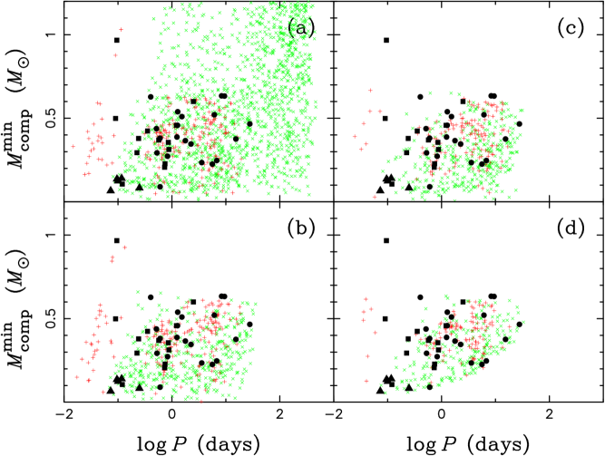
Figure 16: Similar to Figure 13, but for sdB stars with and without selection effects from simulation set 2 (the best-fit model): no selection effects (a), the GK selection effect (b), the GK and the strip selections effects (c), the GK, the strip and the $K$ selection effects (d).

The observed samples of sdB stars are strongly affected by selection effects. These are relatively well defined for the sample of Maxted et al. [2001]. Figure 16 illustrates how the selection effects operate for this sample in the $\log P$ - $M_{\rm comp}^{\rm min}$ diagram and similarly Figures 17 and 18 show the corresponding effects for the distributions of sdB stars in the $T_{\rm eff}$ - $\log g$ diagram and the HRD, respectively (all for simulation 2, our best-fit model). For comparison, Figures 19 and 20 show the distributions in the $T_{\rm eff}$ - $\log g$ diagram and the HRD for the different formation channels to illustrate how the selection effects determine the relative importance of the various channels in observed samples.

The most important selection effect is the GK selection effect which we apply in the following way. If a sdB binary has a MS companion and the effective temperature of the companion is above 4000 K or the companion is brighter than the sdB star, the system is excluded. All sdB binaries from the first stable RLOF are removed in this way in panel (b) of Figure 16 as the companions are too massive (see panel a of Figure 15). The sdB binaries from the first CE ejection channel with MS companion masses larger than $0.60\,M_{\odot}$ for Pop I (or $0.47\,M_{\odot}$ for a thick-disc population) are also removed. The strip effect selects mainly against sdB stars with masses significantly different from $0.5\,M_{\odot}$. This excludes a significant fraction of sdB stars formed through the merger channel since these tend to have fairly high masses. Similarly, sdB stars which formed from CE ejection channels where their progenitor had a ZAMS mass larger than the helium flash mass $M_{0}$ tend to produce sdB stars with small masses and are also likely to be removed by the strip selection criterion (see panel c of Fig. 16). Finally, the $K$ effect selects against sdB stars with long orbital periods and small companion masses. As all the sdB stars with known orbital periods have semi-amplitudes $K$ larger than 30 km s^-1, we therefore remove sdB binaries with $K$ lower than 30 km s^-1 (see panel d of Fig. 16).

Since the GK effect only excludes sdB binaries, it decreases the binary fraction of sdB stars (see Table 2). On the other hand the strip selection effect removes both binary sdB stars and sdB stars from the merger channel. Whether this increases or decreases the binary fraction relative to the consideration of the GK effect alone depends sensitively on the CE ejection parameters. For simulations with relatively low $\alpha_{\rm CE}$ and $\alpha_{\rm th}$, the orbital separations of the resulting helium WD pairs are relatively small leading to a larger merger rate. Since the resulting single sdB stars tend to be relatively massive, they are mostly removed by the strip selection effect.

In our simulations, we did not consider any luminosity selection, as one might expect to be important in a magnitude-limited sample. Figure 12 shows the distributions of the masses of sdB stars from various channels. The first stable RLOF channel produces a large fraction of low-mass sdB stars, which tend to have lower luminosity and should therefore be underrepresented in a magnitude-limited sample. On the other hand, the merger channel produces a large fraction of relatively massive sdB stars which one would be able to detect to larger distances in a magnitude-limited sample.

For reference and comparison we show in Figures 21 to 25 the distributions of orbital period, the mass of the sdB star, mass ratio, mass function and radial-velocity semi-amplitude from all channels for our best-fit model (simulation 2) and show how these distributions are affected by the selection effects.

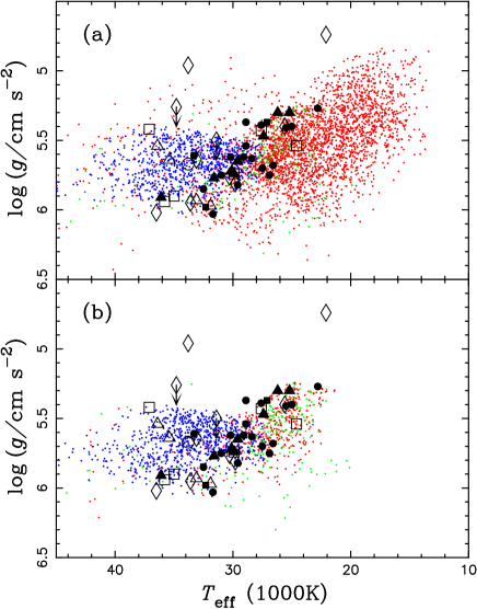
Figure 17: The $T_{\rm eff}$ - $\log g$ diagram for simulation set 2 (the best-fit model). Dots represent the results of the simulation. Filled circles indicate the position of observed sdB binaries with orbital periods $P_{\rm orb}<1\,{\rm d}$, solid triangles binaries with $1<P_{\rm orb}<10\,{\rm d}$, and solid squares binaries with $P_{\rm orb}>10\,{\rm d}$. Circles show systems that have radial velocity variations ${\rm d}V>40\,{\rm km}\,{\rm s}^{-1}$, triangles systems with $20<{\rm d}V<40\,{\rm km}\,{\rm s}^{-1}$, squares systems with $10<{\rm d}V<20\,{\rm km}\,{\rm s}^{-1}$ and diamonds systems with ${\rm d}V<10\,{\rm km}\,{\rm s}^{-1}$, where ${\rm d}V$ is the maximum difference between radial velocities measured for a particular object. Arrows indicate lower limits for $g$. Panel (a) does not include selection effects, while in panel (b) the GK selection effect has been taken into account. sdB stars from the CE ejection channels are assumed to have envelope masses between 0.0 and $0.006\,M_{\odot}$, sdB stars from stable RLOF channels to have envelope masses between 0.0 and $0.012\,M_{\odot}$, and sdB stars from the merger channel to have envelope masses between 0.0 and $0.002\,M_{\odot}$.

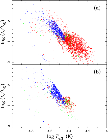
Figure 18: HRD for sdB stars from simulation set 2 (the best-fit model): panel (a) without any selection effect, and panel (b) with the GK selection effect. The model assumptions are the same as in Figure 17.

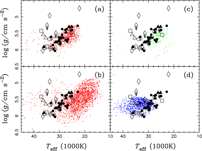
Figure 19: Similar to Figure 17, but for sdB stars from different channels in simulation set 2 - the best-fit model (no selection effects applied). Panels (a), (b), (c) and (d) represent the first CE ejection, the first stable RLOF, the second CE ejection and the merger channel, respectively.

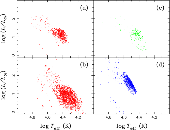
Figure 20: Similar to Figure 18, but for sdB stars from different channels in simulation set 2 - the best-fit model (no selection effects applied). Panels (a), (b), (c) and (d) represent the first CE ejection, the first stable RLOF, the second CE ejection and the merger channel, respectively.

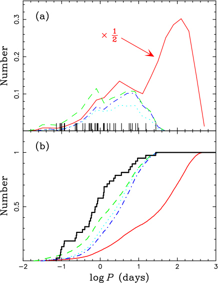
Figure 21: The distribution of orbital periods of sdB stars from all the channels in simulation set 2 - the best-fit model. Panel (a) is a normal distribution while panel (b) shows a cumulative one. Solid curves are for sdB stars without the inclusion of selection effects, while for the dashed curves the GK selection effect has been applied. In the dot-dashed curves, both the GK and the strip selection effects are considered, while for the dotted curves the GK, the strip and the $K$ selection effects are all included. Note that the solid curve in panel (a) has been rescaled by a factor of 1/2 for clarity Short ticks along the X-axis of panel (a) indicate the positions of sdB stars in the sample of Maxted et al. (2001), while the thick histogram represents the observed distribution in panel (b).

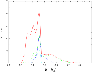
Figure 22: The distribution of masses of sdB stars from all the channels in simulation set 2 (the best-fit model); solid curve: no selection effects; dashed curve: the GK selection effect; dot-dashed curve: the GK and the strip selection effects; dotted curve: the GK, the strip and the $K$ selection effects.

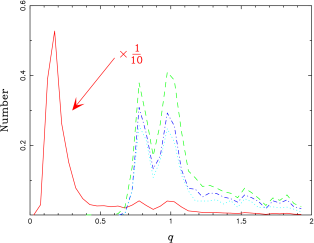
Figure 23: The distribution of mass ratios ($q=M_{\rm sdB}/M_{\rm comp}$) of sdB binaries from all the binary channels in simulation set 2 (the best-fit model) when different selection effects are taken into account: no selection effects (solid); the GK selection effect (dashed); the GK and the strip selection effect (dot-dashed); the GK, the strip and the $K$ selection effect (dotted). Note that the solid curve has been rescaled by a factor of 1/10 for clarity.

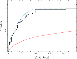
Figure 24: Cumulative distribution of mass functions $f(M)={M_{\rm comp}^{3}(\sin i)^{3}/(M_{\rm sdB}+M_{\rm comp})^{2}}$ of sdB stars from all the channels in simulation set 2 - the best-fit model (where we assume that the normal direction of the orbital plane is uniformly distributed in solid angle). The various curves represent the mass function of sdB stars when various selection effects are taken into account: no selection effects (solid), the GK selection effect (dashed), the GK and strip selection effects (dot-dashed), the GK, strip and K selection effects (dotted). The thick histogram shows the observational distribution of Maxted et al. (2001), Morales-Rueda et al. (2002a,b).

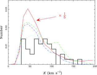
Figure 25: The distribution of the semi-amplitudes $K$ of radial velocities for sdB binaries from all the binary channels in simulation set 2 - the best-fit model (where we assume that the normal direction of the orbital plane is uniformly distributed in solid angle). The solid curve represents sdB stars without any selection effect considered (the line has been rescaled by a factor of 1/5 for clarity), the dashed curve includes the GK selection effect, the dot-dashed curve both the GK and the strip selection effects, and the dotted curve the GK, the strip and the $K$ selection effects. The thick histogram represents the observational sample of Maxted et al. 2001, Morales-Rueda et al. 2002a,b).

7.7 Expected birthrates and total numbers

As Table 1 shows, the predicted birthrate of Pop I sdB stars from all channels is in the range $0.014$ – $0.063\,{\rm yr}^{-1}$ for the whole Galaxy, where our best models (simulations 2 and 8) give a rate of $\sim 0.05\,{\rm yr}^{-1}$. The formation rate from the merger channel alone, which produces single sdB stars, is in the range of 0.003 – $0.017\,{\rm yr}^{-1}$, somewhat lower than the estimate of Tutukov & Yungelson (1990) who obtained a rate of $0.029\,{\rm yr}^{-1}$. By taking an effective Galactic volume of $5\times 10^{11}\,{\rm pc}^{3}$ [1990], this can be converted into an average birthrate per pc³ of $2.8$ – $12.6\times 10^{-14}\,{\rm pc}^{-3}\,{\rm yr}^{-1}$ or $10\times 10^{-14}\,{\rm pc}^{-3}\,{\rm yr}^{-1}$ for the best model. When convolved with the lifetime of the sdB phase, these rates imply a total number of sdB stars in the Galaxy of $2.4\times 10^{6}$ – $9\times 10^{6}$, or a space number density of 0.5 – $1.9\times 10^{-5}\,{\rm pc}^{-3}$, where our best estimates are $\sim 6\times 10^{6}$ and $\sim 1\times 10^{-5}\,{\rm pc}^{-3}$, respectively. Including the GK selection effect reduces both the number and the density of selected sdB stars by about a factor of 2. The inclusion of the strip selection effect further halves these numbers. For a thick-disc population, the birthrate and the total number of sdB stars would be higher than for Pop I if we adopted similar model parameters for both populations (in particular, using the same star-formation rate).

7.8 Comparison with observations

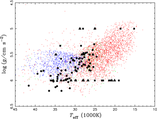
Figure 26: The $T_{\rm eff}$ - $\log g$ diagram for simulation set 2 - the best-fit model. Filled circles show the position of observed sdB stars from Saffer et al. (1994), filled triangles and filled squares represent single and binary sdB stars, respectively, from the observations of Aznar Cuadrado & Jeffery (2001).

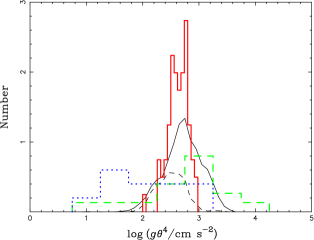
Figure 27: The distribution of $\log(g\theta^{4})$, where $g$ is the surface gravity of a sdB star, and $\theta=5040\,{\rm K}/T_{\rm eff}$. The solid histogram is obtained from the 68 sdB stars observed by Saffer et al. (1994), while the dashed and dotted histograms are based on the observations of 15 sdB stars and 10 sdO stars, respectively, by Ulla & Thejll (1998). The solid curve represents the sdB stars from simulation set 2 (the best-fit model) without consideration of selection effects, while the dashed curve includes the GK selection effect.

Heber [1986] estimated the birthrate of sdB stars to be $\sim 2\times 10^{-14}\,{\rm pc}^{-3}\,{\rm yr}^{-1}$ and the space density to be $\sim 4\times 10^{-6}\,{\rm pc}^{-3}$. Downes [1986] derived a space density of $\sim 2\times 10^{-6}\,{\rm pc}^{-3}$ from observations, while Bixler, Bowyer & Laget [1991] obtained a density of $\sim 3.3\times 10^{-6}\,{\rm pc}^{-3}$. Most other studies gave similar values, although Villeneuve et al. [1995], using a much larger scale height, obtained a birthrate density and a space density which are by a factor of $\sim 5$– 10 lower than the previous estimates, although this would not affect the overall birthrate estimate. The observational estimates are in reasonable agreement with our theoretical estimates, in particular after selection effects have been taken into account.

Observationally, over half of the sdB stars are in binaries with MS/giant companions [1994, 2001]. The sdB stars with MS/giant companions constitute 63 – 88 per cent in our simulations. More than two thirds of the sdB candidates of Maxted et al. [2001] are binaries with short orbital periods. With the GK effect, the sdB binaries with short orbital periods produced from our simulations constitute 41 – 86 per cent of the observable population. In the observational data set of Maxted et al. [2001], 13 of 18 (or 72 per cent) sdB binaries with known companion types have WD companions [2002b], although the majority of sdB stars in the sample are presently of unknown type. The relative number of systems with WD and MS secondaries will allow to further refine the BPS model, in particular $q_{\rm crit}$; however, as we have shown, these numbers are strongly affected by the selection effects.

Figure 17 displays a comparison of our best model (simulation 2) with the observations of Maxted et al. [2001] in the $T_{\rm eff}$ – $\log g$ diagram. The distribution of observed systems (as indicated by large symbols) matches the simulated one (as indicated by dots) quite well after the GK selection effect has been taken into account. PG 1051+501 and PG 1553+273 (the two top diamonds) may originate from the first stable RLOF channel and may have relatively large hydrogen-rich envelopes (see also panel b of Figure 19). In the simulation, sdB stars from the CE ejection channels are assumed to have envelope masses between 0.0 and $0.006\,M_{\odot}$, sdB stars from stable RLOF channels to have envelope masses between 0.0 and $0.012\,M_{\odot}$, and sdB stars from the merger channel to have envelope masses between 0.0 and $0.002\,M_{\odot}$. Brown et al. [2001] pointed out that the envelope composition can be changed dramatically (e.g. from hydrogen-rich to helium-rich) due to helium-flash-induced mixing between the interior and the envelope. The hydrogen mixed into the hot He-burning interior is burned rapidly and the mass of the hydrogen-rich envelope can be reduced. Such mixing is found for sdB stars evolving to steady core helium burning with hydrogen-rich envelopes of masses $\sim 0.0006M_{\odot}$. The mixing may also occur in a binary model and have a small effect on envelope masses, while the assumption on envelope masses is rather ad hoc in the simulation. Figure 26 compares the observations of Saffer et al. [1994] and Aznar Cuadrado & Jeffery [2001] with the sdB stars from our best model (as indicated by dots). Filled circles show the position of observed sdB stars from Saffer et al. [1994], filled triangles and filled squares represent single and binary sdB stars, respectively, from the observation of Aznar Cuadrado & Jeffery [2001]. The candidates of Saffer et al. [1994] were taken from the PG catalogue and therefore suffer from the GK selection effect, while the candidates of Aznar Cuadrado & Jeffery [2001] were taken from the IUE archive and are affected by uncertain selection effects. Aznar Cuadrado & Jeffery [2001] used a grid of high-gravity helium-deficient model atmospheres [1997] to determine the atmospheric parameters. Their grid has a spacing of 2000 K in $T_{\rm eff}$ and a spacing of 0.5 dex in $\log g$. Therefore, the $\log g$ values of their measured sdB stars have only three discreet values: 5.0, 5.5 and 6.0. With these limitations in mind, we conclude that our simulations can reasonably explain their observations.

The distribution of orbital periods of sdB binaries [2001] is explained reasonably well in Figure 21 after the various selection effects have been applied. However, the distribution also suggests that the observed sample may be missing some of the sdB binaries with relatively long orbital periods.

The distribution of the masses of sdB stars from simulation set 2 (the best-fit model) is plotted in Figure 22; note in particular how narrow the mass distribution becomes once selection effects have been taken into account. This also implies that real intrinsic mass distribution of sdB stars should be much wider than the observed one. Since it is difficult to measure the mass directly from observation, we also plot in Figure 27 the distribution of $\log(g\theta^{4})$ (where $\theta=5040{\rm K}/T_{\rm eff}$) for the sdB stars from simulation set 2 and histograms for 68 sdB stars observed by Saffer et al. [1994], 15 sdB stars and 10 sdO stars observed by Ulla & Thejll [1998]. The quantity $g\theta^{4}$ is approximately constant for sdB stars of a given mass (since it is proportional to the mass – luminosity ratio; Greenstein & Sargent 1974, also see Fig. 3 of Paper I), and therefore the distribution of this quantity provides some information on the mass distribution. The distribution from simulation set 2 is consistent with that from Saffer et al. [1994] after inclusion of the GK selection effect and taking into account the fact that some of the sdB stars from simulation set 2 are actually sdO stars. Those sdO stars come from the merger channel and are massive and therefore have low values of $g\theta^{4}$.

The mass-ratio distribution (see Figure 23) has three peaks: the first peak is caused by sdB star from the first stable RLOF channel, the second and the third are due to the bimodal distribution of WD masses in the second CE ejection channel. However, it is the mass function rather than the mass ratio that can be measured directly from observations. The observed mass function distribution (see Figure 24) is well explained after application of the GK selection effect.

Figure 25 gives the distributions of radial-velocity semi-amplitudes $K$ of sdB binaries. The comparison between the theoretical and the observed distributions suggests that some sdB stars with a low value of $K$ are missing in the observed samples.

7.9 Comparison with the results of previous studies

D’Cruz et al. [1996] tried to understand the formation of sdB stars by employing and varying the Reimers mass-loss formula near the tip of the FGB. In their picture, it was a stellar wind that peeled off the hydrogen envelope of a FGB star before helium ignition, which then occurred at much higher $T_{\rm eff}$ leading to the formation of a sdB star. They assumed a broad distribution in the Reimers coefficient $\eta$ in order to explain the observations. The value of $\eta$ has to be 2 – 3 times larger in some stars to produce sdB stars than to produce normal horizontal-branch stars. At present, there is no theoretical justification for such a range of $\eta$ values for single stars. On the other hand, our model provides a natural way to produce sdB stars without tuning the Reimers coefficient. Binary interactions naturally expose the hydrogen-exhausted cores of FGB stars either by stable RLOF or CE ejection. An enhanced wind, as required by D’Cruz et al. [1996], may be possible in binary systems since the stellar wind may be tidally enhanced due to the proximity of a companion star [1989, 1995]. sdB stars produced in this way would be binaries with relatively long orbital periods. We have not included a tidally enhanced stellar wind since we did not want to introduce further uncertainties into the modelling. Nevertheless, this channel certainly needs to be studied further even though the channel may ultimately turn out not to be very significant since it probably requires significant fine-tuning of the stellar wind parameters (i.e. it requires a fairly narrow range of binary separations).

Webbink [1984], Iben & Tutukov [1986], Tutukov & Yungelson (1990) and Iben et al. (1997) have investigated in detail the merger channel for the formation of sdB stars. Their most recent estimate (Iben et al. 1997) for the merger rate of helium WDs in the Galaxy is $\sim 0.02\,{\rm yr}^{-1}$, which is quite similar to our estimate of 0.003 – $0.017\,{\rm yr}^{-1}$. Iben et al. [1997] did not specifically examine whether the merger product would ignite helium and hence become a sdB star. Nevertheless, their results are consistent with ours, since we found in our simulations that in fact most merger products of helium WD pairs ignite helium. Han [1998] gave a birthrate of 0.002 – $0.014\,{\rm yr}^{-1}$ in his study on the formation of double degenerates. Our new birthrate is slightly larger than his, mainly because we adopted a higher value for $q_{\rm crit}$ for the first stable RLOF phase, which makes the second CE ejection channel more likely and ultimately increases the merger rate. The distribution of masses of helium WD mergers in the present paper (see Fig. 12) is similar to the distribution in Figure 6 of Han (1998).

Mengel, Norris & Gross [1976] have modelled the conservative evolution of a binary system with initial masses of $0.80\,M_{\odot}$ and $0.78\,M_{\odot}$ for the primary and the secondary, respectively, for a composition with $X=0.73$ and $Z=0.001$. They also found that there is a range of initial separations for which a sdB star is formed as a result of stable and conservative RLOF. The sdB star formed in their calculations had a mass $\sim 0.5\,M_{\odot}$ and an orbital period of $\sim 300\,{\rm d}$. Both the mass and the period fall inside the range of sdB stars from the first stable RLOF channel in our simulations although we use higher metallicities and assume non-conservative mass transfer.

7.10 Further observational tests to the model

In this paper we used the well-defined sample of sdB stars of Maxted et al. [2001] and Morales-Rueda et al. (2002a,b) to calibrate our BPS model. However, because of the design of the sample and various selection effects, it only comprises a subset of the whole population of sdB stars included in the BPS model. Hence our model can be used to make predictions about the wider population of sdB stars. Extending the observational sample should then allow to test these predictions and to help refine some of the BPS parameters that are presently not well constrained.

As one can see from Figures 17 and 19, there are a few observed sdB stars (in fact sdO stars) with $\log g\sim 5.75$ and $T_{\rm eff}\sim 40000\,{\rm K}$. Their position in the $T_{\rm eff}$ – $\log g$ suggests that they are more massive than $\sim 0.5\,M_{\odot}$ (see Fig. 2d of Paper I). Since the GK selection effect tends to eliminate sdB stars from the first stable RLOF channel, most of these are likely to be single sdB stars formed from the merger channel (although one of them, PG0839+399, is a binary with an orbital period of 5.622 d).

Our model predicts that a large fraction, perhaps the majority of the intrinsic population of sdB stars have MS companions. In particular, Figure 15 shows that sdB stars from the first stable RLOF can have companions with a spectral type as early as B. The predicted numbers of sdB stars with B, A or F type companions in the Galaxy at the current epoch are 0.69, 2.4, 0.89 million, respectively, for simulation set 2 (our best-fit model with $q_{\rm crit}=1.5$) or 0.50, 0.61, 0.56 million for simulation set 8 (with $q_{\rm crit}=1.2$). The numbers of B, A, or F type stars in the Galaxy at the current epoch are 34, 314, 1898 million, respectively, in our BPS model. These numbers imply that 2.0 per cent of B type stars, 0.75 per cent of A type stars and 0.047 per cent of F type stars should have sdB companions, respectively, for simulation set 2. For simulation set 8, the corresponding numbers are 1.4 per cent for B type stars, 0.19 per cent for A type stars and 0.030 per cent for F type stars. The main difference between simulation sets 2 and 8 is the value of $q_{\rm crit}$ (1.5 in set 2 and 1.2 in set 8). These percentages demonstrate (also see the discussion in section 7.5) that the percentage of A type stars with sdB companions is quite sensitive to $q_{\rm crit}$, the critical mass ratio above which mass transfer is dynamically unstable on the FGB or AGB (The sensitivity is due to the fact that such systems have experienced stable RLOF on the FGB). Observations of A type stars with sdB companions may therefore help to constrain $q_{\rm crit}$, a basic and important parameter in any BPS model.

8 Conclusion

In this paper we have presented a comprehensive BPS study for the formation of sdB stars and investigated the importance of the various evolutionary channels that lead to the formation of sdB stars. We studied the roles of both the theoretical model parameters and the observational selection effects. We obtained birthrates for sdB stars of 0.014 – 0.063 $\,{\rm yr}^{-1}$, a total number of sdB stars in the Galaxy of 2.4 – 9.5 million and a sdB binary fraction of 76 – 89 per cent. The distribution of orbital periods ranges from 0.5 hr to 500 d, possibly with three peaks at $\sim 2.4$ hr, $\sim 2$ d and $\sim 100$ d. The distribution of masses has a fairly wide range from $0.3\,M_{\odot}$ to $0.8\,M_{\odot}$ with a major peak near $0.46\,M_{\odot}$.

Comparing our simulations to observed samples of sdB stars, we found a best-fit model that explains the observed distribution quite satisfactorily with very reasonable theoretical parameters. Based on this best-fit model, we conclude:

1. The first RLOF needs to be more stable for a wider range of parameters than is commonly assumed, either because of a higher critical mass ratio $q_{\rm crit}$ for the occurrence of dynamical mass transfer or a tidally enhanced stellar wind. This suggests that the criterion for stable RLOF needs to be studied further.

2. The first stable RLOF is non-conservative, and the mass lost from the system carries away a specific angular momentum similar to that of the system.

3. In agreement with earlier studies, we find that the common-envelope ejection is a very efficient process, though the values of $\alpha_{\rm CE}$ and $\alpha_{\rm th}$ cannot yet be precisely determined.

4. Our best model explains the observed properties of sdB stars quite satisfactorily (in particular, the $\log P$ – $M_{\rm comp}$ diagram, the $T_{\rm eff}$ – $\log g$ diagram, the orbital period distribution, the $\log(g\theta^{4})$ distribution, the mass function distribution, the binary fraction of sdB stars, the birth rates, the space number densities etc.).

5. Our best-fit model predicts a much wider distribution of masses for sdB stars than is commonly assumed. It also predicts that some B, A and F type stars have sdB companions and that the percentage of A type stars with sdB companions can be used to constrain the critical mass ratio for stable RLOF on the FGB.

References

- [1994] Allard F., Wesemael F., Fontaine G., Bergeron P., Lamontagne R., 1994, AJ, 107, 1565
- [2001] Aznar Cuadrado R., Jeffery C.S., 2001, A&A, 368, 994
- [2000] Billéres M., Fontaine G., Brassard P., et al. 2000, ApJ, 530, 441
- [1991] Bixler J.V., Bowyer S., Laget M., 1991, A&A, 250, 370
- [] Brassard P., Fontaine G., Billéres M., Charpinet S., Liebert J., Saffer R.A., 2001, ApJ, 305, 228
- [1997] Brown T.M., Ferguson H.C., Davidsen A.F., Dorman B., 1997, ApJ, 482, 685
- [2001] Brown T.M., Sweigart A.V., Lanz T., Landsman W.B., Hubeny I., 2001, ApJ, 562, 368
- [1996] Carraro G., Girardi L., Bressan A., Chiosi C., 1996, A&A, 305, 849
- [2002] Chen X., Han Z., 2002, MNRAS, 335, 948
- [1996] D’Cruz N.L., Dorman B., Rood R.T., O’Connell R.W., 1996, ApJ, 466, 359
- [2000] Dewi J., Tauris T., 2000, A&A, 360, 1043
- [1986] Downes R.A., 1986, ApJS, 61, 569
- [2002] Drechsel H., Heber U., Napiwotzki R., et al. 2002, A&A, in press
- [1989] Eggleton P.P., Fitchett M.J., Tout C.A., 1989, ApJ, 347, 998
- [1989] Eggleton P.P., Tout C.A., 1989, in Batten A.H., ed., Algols, Kluwer, Dordrecht, p. 164
- [1984] Ferguson D.H., Green R.F., Liebert J., 1984, ApJ, 287, 320
- [1994] Goldberg D., Mazeh T., 1994, A&A, 282, 801
- [1986] Green R.F., Schmidt M., Liebert J., 1986, ApJS, 61, 305
- [1974] Greenstein J.L., Sargent A.I., 1974, ApJS, 28, 157
- [1995] Han Z., 1995a, Ph.D. Thesis (Cambridge)
- [1998] Han Z., 1998, MNRAS, 296, 1019
- [1995] Han Z., Eggleton P.P., Podsiadlowski Ph., Tout C.A., 1995b, MNRAS, 277, 1443
- [2001] Han Z., Eggleton P.P., Podsiadlowski Ph., Tout C.A., Webbink R.F., 2001, in Podsiadlowski Ph., Rappaport S., King A.R., D’Antona F., Burderi L., eds, Evolution of Binary and Multiple Star Systems, ASP Conf. Ser., Vol. 229, p. 205
- [1994] Han Z., Podsiadlowski Ph., Eggleton P.P., 1994, MNRAS, 270, 121 (HPE)
- [1995] Han Z., Podsiadlowski Ph., Eggleton P.P., 1995, MNRAS, 272, 800
- [2002] Han Z., Podsiadlowski Ph., Maxted P.F.L., Marsh T.R., Ivanova N., 2002, MNRAS, 336, 449 (Paper I)
- [2000] Han Z., Tout C.A., Eggleton P.P., 2000, MNRAS, 319, 215
- [1999] Han Z., Webbink R.F., 1999, A&A, 349, L17
- [1986] Heber U., 1986, A&A, 155, 33
- [2002] Heber U., Moehler S., Napiwotzki R., Thejll P., Green E.M., 2002, A&A, 383, 938
- [1987] Hjellming M.S., Webbink R.F., 1987, ApJ, 318, 794
- [1983] Iben I. Jr., Renzini A., 1983, ARA&A, 21, 271
- [1986] Iben I. Jr., Tutukov A.V., 1986, ApJ, 311, 753
- [1997] Iben I. Jr., Tutukov A.V., Yungelson L.R., 1997, ApJ, 475, 291
- [1998] Jeffery C.S., Pollacco D.L., 1998, MNRAS, 298, 179
- [1988] Kilkenny D., Heber U., Drilling J.S., 1988, South African Astronomical Observatory Circulars, No. 12
- [1999] Kilkenny D., Koen C., Jeffery J., Hill C.S., O’Donoghue D., 1999, MNRAS, 310, 1119
- [1997] Kilkenny D., Koen C., O’Donoghue D., Stobie R.S., 1997, MNRAS, 285, 640
- [1993] Kroupa P., Tout C.A., Gilmore G., 1993, MNRAS, 262, 545
- [1998] Koen C., Orosz J.A., Wade R.A., 1998, MNRAS, 300, 695
- [2000] Maxted P.F.L., Moran C.K.J., Marsh T.R., Gatti A.A., 2000, MNRAS, 311, 877
- [2000] Maxted P.R.L., Marsh T.R., North R.C., 2000, MNRAS, 317, L41
- [2001] Maxted P.F.L., Heber U., Marsh T.R., North R.C., 2001, MNRAS, 326, 1391
- [1992] Mazeh T., Goldberg D., Duquennoy A., Mayor M., 1992, ApJ, 401, 265
- [1976] Mengel J.G., Norris J., Gross P.G., 1976, ApJ, 204, 488
- [1979] Miller G.E., Scalo J.M., 1979, ApJS, 41, 513
- [2002a] Morales-Rueda L., Marsh T.R., North R.C., Maxted P.F.L., 2002a, Proceedings of the 13th European Meeting on White Dwarfs, in press
- [2002b] Morales-Rueda L., Maxted P.F.L., Marsh T.R., North R.C., Heber U., 2002b, MNRAS, in press (astro-ph/0209472)
- [1999] Moran C., Maxted P., Marsh T.R., Saffer R.A., Livio M., 1999, MNRAS, 304, 535
- [2001] Napiwotzki R., Edelmann H., Heber U., et al. , 2001, A&A, 378, L17
- [1997] O’Donoghue D., Lynas-Gray A.E., Kilkenny D., et al. 1997, MNRAS, 285, 657
- [1999] Orosz J.A., Wade R.A., 1999, MNRAS, 310, 773
- [1965] Paczyński B., 1965, Acta Astron., 15, 89
- [1976] Paczyński B., 1976, in Eggleton P.P., Mitton S., Whelan J., eds, Structure and Evolution of Close Binaries, Kluwer, Dordrecht, p. 75
- [1969] Paczyński B., Ziółkowski J., Żytkow A., 1969, in Hack M. ed., Mass Loss from Stars, Reidel, Dordrecht, P. 237
- [1973] Plavec M., Ulrich R.K., Polidan R.S., 1973, PASP, 85, 769
- [2002] Podsiadlowski Ph, Han Z., Rappaport S., 2002, MNRAS, submitted
- [1992] Podsiadlowski Ph., Joss P.C, Hsu J.J.L., 1992, ApJ, 391, 246 (PJH)
- [1983] Rappaport S., Verbunt F., Joss P.C., 1983, ApJ, 275, 713
- [] Reimers D., 1975, Mem. R. Soc. Liège, 6ième Serie, 8, 369
- [1981] Renzini A., 1981, in Effects of Mass Loss on Stellar Evolution, ed. C. Chiosi & R. Stalio (Dordrecht: Reidel), 319
- [1994] Saffer R.A., Bergeron P., Koester D., Liebert J., 1994, ApJ, 432, 351
- [1998] Saffer R.A., Livio M., Yungelson L.R., 1998, ApJ, 502, 394
- [2000] Saio H., Jeffery C.S., 2000, MNRAS, 313, 671
- [1997] Soberman G.E., Phinney E.S., van den Heuvel E.P.J., 1997, A&A, 327, 620
- [] Soker N., Harpaz A., 2002, submitted (astro-ph/0209141)
- [1997] Sweigart A.V., 1997, ApJ, 474, L23
- [1995] Thejll P., Ulla A., MacDonald J., 1995, A&A, 303, 773
- [1988] Tout C.A., Eggleton P.P., 1988, MNRAS, 231, 823
- [] Tutukov A.V., Yungelson L.R., 1990, A.Zh., 67, 109
- [1998] Ulla A., Thejll P., 1998, A&AS, 132, 1
- [1987] Vauclair G., Liebert J., 1987, in Y. Kondo ed., Exploring the Universe with the IUE Satellite, Dordrecht, Reidel, p. 355
- [1981] Verbunt F., Zwaan C., 1981, A&A, 100, L7
- [1995] Villeneuve B., Wesemael F., Fontaine G., Carignan C., Green R.F., 1995, ApJ, 446, 646
- [1984] Webbink R.F., 1984, ApJ, 277, 355
- [1988] Webbink R. F., 1988, in Mikołajewska J., Friedjung M., Kenyon S. J., Viotti R., eds, The Symbiotic Phenomenon. Kluwer, Dordrecht, p. 311
- [1999] Wood J.H., Saffer R., 1999, MNRAS, 305, 820
- [1997] Yi S., Demarque P., Oemler A. Jr., 1997, ApJ, 486, 201
- [1999] Yi S., Lee Y., Woo J., Park J., Demarque P., Oemler A.Jr., 1999, ApJ, 513, 128
- [2000] Zoccali M., Cassisi S., Frogel J.A., et al. 2000, ApJ, 530, 418
- [1990] Zombeck M.V., 1990, Handbook of Astronomy and Astrophysics, Second Edition, Cambridge, UK, Cambridge University Press