The ESO-Sculptor Survey: Luminosity functions of galaxies per spectral type at redshifts $0.1-0.5$

We present the first statistical analysis of the complete ESO-Sculptor Survey (ESS) of faint galaxies. The flux-calibrated sample of 617 galaxies with $R_{\mathrm{c}}\leq 20.5$ is separated into 3 spectral classes, based on a principal component analysis which provides a continuous and template-independent spectral classification. We use an original method to estimate accurate K-corrections: comparison of the ESS spectra with a spectral library using the principal component analysis allows us to extrapolate the missing parts of the observed spectra at blue wavelengths, then providing a polynomial parameterization of K-corrections as a function of spectral type and redshift. We also report on all sources of random and systematic errors which affect the spectral classification, the K-corrections, and the resulting absolute magnitudes.

We use the absolute magnitudes to measure the Johnson-Cousins $B$, $V$, $R_{\mathrm{c}}$ luminosity functions of the ESS as a function of spectral class. The shape of the derived luminosity functions show marked differences among the 3 spectral classes, which are common to the $B$, $V$, $R_{\mathrm{c}}$ bands, and therefore reflect a physical phenomenon: for galaxies of later spectral type, the characteristic magnitude is fainter and the faint-end is steeper. The ESS also provides the first estimates of luminosity functions per spectral type in the $V$ band.

The salient results are obtained by fitting the ESS luminosity functions with composite functions based on the intrinsic luminosity functions per morphological type measured locally by Sandage et al. (1985) and Jerjen & Tammann (1997). The Gaussian luminosity functions for the nearby Spiral galaxies can be reconciled with the ESS intermediate and late-type luminosity functions if the corresponding classes contain an additional Schechter contribution from Spheroidal and Irregular dwarf galaxies, respectively. The present analysis of the ESS luminosity functions offers a renewed interpretation of the galaxy luminosity function from redshift surveys. It also illustrates how luminosity functions per spectral type may be affected by morphological type mixing, and emphasizes the need for a quantitative morphological classification at $z\ga 0.1$ which separates the giant and dwarf galaxy populations.

1 Introduction

The galaxy luminosity function (LF hereafter) is a fundamental measure for characterizing the large-scale galaxy distribution. In the current models of galaxy formation based on gravitational clustering, the LF provides constraints on the mechanisms for the formation of galaxies within the dark matter halos (Cole et al., 2000; Baugh et al., 2002). The bulge-dominated and disk-dominated galaxies can be traced separately in the models and compared directly with the observations (Baugh et al., 1996; Kauffmann et al., 1997; Cole et al., 2000). Nevertheless, due to the necessary compromise between a large statistical volume and sufficient resolution for simulating the individual galaxies, the N-body models only describe a limited range of galaxy masses and morphological types (Mathis et al., 2002). In contrast, observational studies of the local galaxy distribution reveal a wealth of details. The galaxy LF spans more than 12 magnitudes (that is 5 orders of magnitude in luminosity; see for example Flint et al. 2001b; Trentham & Tully 2002). Moreover, each morphological type has a distinct LF, denoted “intrinsic” LF, with different parametric functions for the giant and dwarf galaxies (see the review by Binggeli et al., 1988). The “general” galaxy LF, averaged over all galaxy types, is then a composite of the intrinsic LFs.

Specific studies of local galaxy concentrations have allowed detailed insight into the intrinsic LFs per galaxy type. Co-addition of the intrinsic LFs for the Virgo cluster (Sandage et al., 1985), the Centaurus cluster (Jerjen & Tammann, 1997), and the Fornax cluster (Ferguson & Sandage, 1991) shows that the giant galaxies have Gaussian LFs, which are thus bounded at bright and faint magnitudes, with the Elliptical LF skewed towards faint magnitudes. Andreon (1998) also shows that the LFs for giant galaxies are invariant in shape among the Virgo, Centaurus and Coma cluster; because these 3 clusters span a wide range of cluster richness, the analysis suggests that these LFs may be universal among galaxy concentrations. In contrast, the LFs for dwarf galaxies may be ever increasing at faint magnitudes to the limit of the existing surveys, with a steeper increase for the dwarf Elliptical galaxies (dE), when compared with the dwarf Irregular galaxies (dI). Schaeffer & Silk (1988) have proposed an analytical description for the bimodal behavior of the galaxy LF, which models the effect of the galaxy binding energy onto the gas and the resulting efficiency in star formation as a function of galaxy mass.

Because of the different intrinsic LFs for giant and dwarf galaxies, the “general” LF in the local group and in nearby clusters and groups has a varying faint-end behavior with the richness of the concentration: this can be partly interpreted in terms of the varying dwarf-to-giant galaxy ratio dE/E which increases with local density (Ferguson & Sandage, 1991; Trentham & Hodgkin, 2002; see also Trentham & Tully 2002). The faint-end behavior of the dE and dI LFs is however still controversial. Slopes as steep as $\alpha\sim-1.3$ are measured for the Spheroidal/red dwarf galaxies in groups en clusters (Ferguson & Sandage, 1991; Andreon & Cuillandre, 2002; Conselice et al., 2002), whereas other less rich environments yield $-1.2\la\alpha\la-1.1$ (Pritchet & van den Bergh, 1999; Flint et al., 2001b; Trentham et al., 2001; Trentham & Tully, 2002), with some significant contribution from the dI galaxies in Trentham et al. (2001). It is unclear whether these differences are solely due to differences in the detected dwarf populations (related to the ratio of dE to dI galaxies), or to the different environments in terms of local density, or to both.

In parallel, measurements of LF per galaxy type have been obtained from systematic redshift surveys, with significant variations from survey to survey. Estimates of intrinsic LFs using visual morphological classification have been obtained from the “nearby” redshift surveys ($z\la 0.1$), based on photographic catalogues (Efstathiou et al., 1988; Loveday et al., 1992; Marzke et al., 1994, 1998; Marinoni et al., 1999). At $z\ga 0.1$, visual morphological classification however becomes highly uncertain and has been replaced by spectral classification (Heyl et al., 1997; Bromley et al., 1998; Lin et al., 1999; Folkes et al., 1999; Fried et al., 2001; Madgwick et al., 2002; Wolf et al., 2003). When neither morphological nor spectral classification are available, the intrinsic LFs are estimated using samples separated by color (Lilly et al., 1995; Lin et al., 1997; Metcalfe et al., 1998; Brown et al., 2001) or the strength of the emission-lines (Lin et al., 1996; Small et al., 1997; Zucca et al., 1997; Loveday et al., 1999). However, none of the existing redshift surveys separate the giant and dwarf galaxy populations, despite the markedly different intrinsic LFs for these 2 populations (Sandage et al., 1985; Ferguson & Sandage, 1991; Jerjen & Tammann, 1997).

In view of the discrepancy between the local measures of the intrinsic LFs and the estimates from redshift surveys at larger distance, we propose here a new approach for reconciling the various LFs. It is based on the LFs per galaxy type measured from the ESO-Sculptor Survey (ESS hereafter). The ESS has the advantage to provide a nearly complete redshift survey of galaxies at $z\la 0.5$ over a contiguous area of the sky (Bellanger et al., 1995), supplemented by CCD-based photometry (Arnouts et al., 1997) and a detailed spectral classification (Galaz & de Lapparent, 1998).

Sect. 2 gathers the analyses used to build the ESS database: Sect. 2.1 describes the spectroscopic sample selection; Sect. 2.2 summarizes the results of the spectral classification analysis, the classification technique itself being reported in details elsewhere (Galaz & de Lapparent, 1998); Sect. 2.3 describes the original method used for deriving K-corrections for the ESS spectra; Sect. 2.4 reports on all sources of random and systematic errors which affect the spectral classification and the derived absolute magnitudes in the ESS catalogue; Sect. 2.5 describes the choice of the spectral classes on which are based the LF calculations.

We then comment on the technique for deriving the ESS LFs in Sect. 3.1; the results are reported and discussed in Sects. 3.2 and 3.3; in Sect. 3.4, we compare the ESS intrinsic LFs with those from the CNOC2 (Lin et al., 1999), the other existing redshift survey to similar redshifts and with spectral classification. In Sect. 4, we then propose a new approach for interpreting the intrinsic LFs from redshift surveys. In Sect. 4.1, we first review the local measurements of intrinsic LFs as a function of morphological type , and we derive the required magnitude conversions for application to the ESS. In Sect. 4.2, we propose composite fits of the ESS intrinsic LFs which are based on the local LFs for giant and dwarf galaxies; we discuss these composite fits for the ESS early, intermediate, and late-type LFs in Sects. 4.3, 4.4, and 4.5 resp. Sect. 4.6 provides further evidence for the presence of dwarf galaxy populations in the ESS, using the distribution of peak surface brightness. Finally, we summarize the results and discuss the prospects raised by the present analysis in Sect. 5.

2 The ESS spectroscopic survey

The goal of the ESO-Sculptor Survey was to produce a complete photometric and spectroscopic survey of galaxies with the following scientific objectives: (i) to map the galaxy distribution of galaxies at $z\simeq 0.1-0.5$ and (ii) to provide a database for studying the variations in the spectro-photometric properties of distant galaxies as a function of redshift and local environment. The ESO-Sculptor Survey was successfully completed as an ESO key-programme, thanks to a guaranteed allocation of $\sim 60$ clear nights of telescope time on the ESO 3.6m and the NTT, performed over a period of 7 subsequent years.

2.1 Sample selection

The ESS photometric survey provides magnitudes in the Johnson $B$, $V$ and the Cousins $R_{\mathrm{c}}$ standard filters, for nearly 13000 galaxies to $V\simeq 24$ over a contiguous rectangular area of $\sim 0.37$ deg² [$1.53^{\circ}\mathrm{(R{.}A{.})}\times 0.24^{\circ}\mathrm{(DEC{.})}$] (Arnouts et al., 1997). The survey region is centered at $\sim 0^{\mathrm{h}}22^{\mathrm{m}}$ (R.A.) $\sim-30^{\circ}06^{\prime}$ (DEC.) in J2000 coordinates, which is located near the Southern Galactic Pole. Multi-slit spectroscopy of the galaxies with $R_{\mathrm{c}}\leq 20.5$ (Bellanger et al., 1995) provided a nearly complete redshift survey over a contiguous sub-area of $\sim 0.25$ deg² [$1.02^{\circ}\mathrm{(R{.}A{.})}\times 0.24^{\circ}\mathrm{(DEC{.})}$]. Selection of the galaxies to be observed spectroscopically was solely based on their $R_{\mathrm{c}}$ magnitude. Crowding on the mask left nearly 6% of the galaxies with $R_{\mathrm{c}}\leq 20.5$ unobserved. Instead, fainter galaxies could be observed where there was remaining space on the multi-slit masks. As a result, the $R_{\mathrm{c}}$ completeness of the ESS spectroscopic catalogue is not a pure step function.

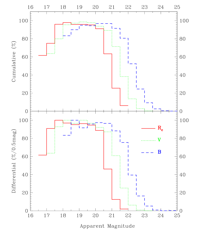
Figure 1: Fractional and cumulative completeness for the ESO-Sculptor spectroscopic catalog, as a function of apparent magnitude, in the Johnson $B$, $V$ and Cousins $R_{\mathrm{c}}$ bands.

Table 1: Differential completeness of the ESO-Sculptor redshift survey in the Johnson $B$, $V$ and Cousins $R_{\mathrm{c}}$ bands.

$R_{\mathrm{c}}$
mag intervala	$\leq 20.0$	$20.0-$20.5	$20.5-21.0$	$21.0-21.5$	$21.5-22.0$
completenessb	94.40 %	92.23 (88.76) %	75.52 (46.19) %	52.28 (12.54) %	34.36 (1.96) %
galaxies with z c	388	617 (229)	793 (176)	870 (77)	888 (18)
$V$
mag interval	$\leq 20.0$	$20.0-20.5$	$20.5-$ 21.0	$21.0-21.5$	$21.5-22.0$	$22.0-22.5$
completeness	95.41 %	94.03 (92.09) %	91.45 (87.19) %	80.40 (60.86) %	59.24 (25.10) %	39.53 (6.30) %
galaxies with z	187	315 (128)	492 (177)	677 (185)	808 (131)	859 (51)
$B$
mag interval	$\leq 21.0$	$21.0-21.5$	$21.5-$ 22.0	$22.0-22.5$	$22.5-23.0$	$23.0-23.5$
completeness	95.60 %	92.48 (88.32) %	85.77 (75.48) %	66.67 (39.46) %	45.10 (16.34) %	28.16 (5.25) %
galaxies with z	174	295 (121)	452 (157)	598 (146)	708 (110)	769 (61)

• Apparent magnitude interval considered for the completeness calculation.

• Cumulated completeness at the faintest limit of the quoted apparent magnitude interval, calculated as the ratio of the number of galaxies with redshift by the number of galaxies in the photometric catalogue; in parentheses is indicated the differential completeness in the quoted apparent magnitude interval.

• Cumulated number of galaxies with a redshift measurement brighter than the faintest limit of the quoted apparent magnitude interval; in parentheses is indicated the differential number of galaxies with a redshift measurement in the quoted apparent magnitude interval.

Figure 1 and Table 1 show the differential and cumulative redshift completeness in the $B$ $V$ $R_{\mathrm{c}}$ bands, in half-magnitude intervals. Table 1 shows that the differential completeness in $R_{\mathrm{c}}$ is nearly flat from bright magnitudes to $R_{\mathrm{c}}=20.0$, with a differential completeness larger than $94\%$, and decreases to 88.76% in the magnitude interval $20.0-20.5$, due to the increase in the surface density of galaxies with magnitude; it then sharply drops to 46%, 13% and 2% in the $R_{\mathrm{c}}$ intervals $20.5-21.0$, $21.0-21.5$, $21.5-22.0$ respectively. Despite the selection of the spectroscopic sample in the $R_{\mathrm{c}}$ band, and the spread in $B-R_{\mathrm{c}}$ and $V-R_{\mathrm{c}}$ colors (see right panels of Fig. 5 in Sect. 2.3), the completeness functions in the $V$ and $B$ bands have a similar behavior to that in $R_{\mathrm{c}}$.

For calculation of the LF in each band, we define a “nominal magnitude limit” as the magnitude limit which provides the best compromise between completeness, small color biases and sufficient statistic. In the $R_{\mathrm{c}}$ band, the choice is obvious and is at $R_{\mathrm{c}}\leq 20.5$, the spectroscopic selection limit (there is no known color bias in the $R_{\mathrm{c}}$ sample at this limit). Due to the spectroscopic selection in the $R_{\mathrm{c}}$ band, the $V$ and $B$ samples are deficient in objects with blue colors at faint magnitudes. We choose the nominal limits at $V\leq 21.0$ and $B\leq 22.0$ resp., for the following reasons:

• the differential completeness is larger than $70\%$ in both the $B$ and $V$ samples at these limits (see Table 1);

• the $B$ and $V$ samples contain a sufficient number of galaxies for calculating intrinsic LFs based on 3 spectral classes;

• the resulting combination of $B$, $V$, and $R_{\mathrm{c}}$ magnitude limits is in agreement with the typical colors of the ESS galaxies at $R_{\mathrm{c}}\simeq 20.5$ ($B-R_{\mathrm{c}}\simeq 1.5$ and $V-R_{\mathrm{c}}\simeq 0.5$, Arnouts et al. 1997).

We show in Sect. 3.2 that the LFs in the $B$ and $V$ bands vary systematically when going to fainter limits than the nominal magnitudes $V\leq 21.0$ and $B\leq 22.0$, due to the increasing color biases at faint magnitudes in these samples. Comparison with the LFs for the $R_{\mathrm{c}}$ sample show that at the chosen $V$ and $B$ nominal limits, the color biases might nevertheless be comparable with the random errors (see Sect. 3.2 and Table 2). By choosing brighter nominal magnitude limits in the $V$ and $B$ bands, one would reduce the color biases in these samples; this would however significantly reduce the number of galaxies (see Table 1), and would not allow us to extract spectral-type LFs in these filters.

As shown by Disney & Phillipps (1983), redshift surveys limited in apparent magnitude also suffer selection effects in the central surface brightness of galaxies. In the ESS photometric catalogue, the surface brightness threshold in object detection used for the SExtractor image analyses (Bertin & Arnouts, 1996) is in the interval $\sim 25.5-26.5$ mag arcsec^-2 in the $R_{\mathrm{c}}$ band, $\sim 25.5-27.0$ mag arcsec^-2 in the $V$ band, and $\sim 26.0-27.5$ mag arcsec^-2 in the $B$ band (the $1$ to $1.5^{\mathrm{mag}}$ intervals are due to variations in the depth of the individual images; most of it is caused by the marked increase in depth when changing from the 3.6m telescope to the NTT; a smaller part is due to the varying sky transparency with time). Due to redshift dimming (see Sect. 4.6), and to a minor extent to K-corrections (see Sect. 2.3), the resulting rest-frame limiting peak surface brightness in the ESS redshift survey is $\leavevmode\nobreak\ 22.0$ mag arcsec^-2 in $R_{\mathrm{c}}$ for galaxies with $R_{\mathrm{c}}\la 21.5$ (see Fig. 13), $\leavevmode\nobreak\ 22.5$ mag arcsec^-2 in $V$ for galaxies with $V\la 22.5$, and $\leavevmode\nobreak\ 23.0$ mag arcsec^-2 in $B$ for galaxies with $B\la 23.5$ (see Sect. 4.6 for definition of ESS peak surface brightness). The ESS distributions of rest-frame peak surface brightness show no or weak correlation with apparent magnitude, indicating that redshift effects have been appropriately corrected for.

McGaugh et al. (1995) show that the low surface brightness population sets in at a central surface brightness fainter than $\sim 22.0$ mag arcsec^-2 in $B$. The ESS spectroscopic sample reaches one magnitude fainter in $B$, therefore detecting a fraction of this population (see also Sects. 4.4 and 4.5). A significant number of low surface brightness galaxies may nevertheless have been missed in the ESS. As shown by McGaugh (1996) and Dalcanton (1998, see also ), the relatively bright threshold in central surface brightness inherent to redshift surveys may significantly affect the luminosity function at both the bright and faint end. Although low surface brightness galaxies may be as numerous as the “normal” galaxies, they however contribute for less than a factor 3 to the luminosity density (McGaugh, 1996; Dalcanton et al., 1997). We show in Sect. 4.6 that the faintest $R_{\mathrm{c}}$ detected galaxies in the ESS also have a low central surface brightness, with no evidence for intrinsically bright though very extended galaxies above the sample limits.

2.2 Spectral classification

Morphological types are not available for the ESS redshift survey. As the survey describes the redshift range $0.1\la z\la 0.6$, a large fraction of the galaxies have diameters smaller than 10 arcseconds, and identification of their morphology is severely limited by the ground-based image quality (see Arnouts et al., 1997). We have therefore chosen to perform the estimation of the intrinsic LFs based on a spectral classification. Galaz & de Lapparent (1998) show that using the ESS data, a spectral classification method based on a Principal Component Analysis (PCA hereafter) provides an objective spectral sequence, which can be parameterized continuously using one or more parameters, and is strongly related to the Hubble sequence of normal galaxies (see also Folkes et al., 1996; Bromley et al., 1998; Baldi et al., 2001).

The PCA allows us to describe each spectrum (in rest-wavelength) as a linear combination of a reduced number of principal vectors, the eigenvectors, also called principal components (PC hereafter), and denoted $PC_{i}$. The PCs better discriminate the whole sample, and bear decreasing variance with increasing index $i$. We denote $\alpha_{i}$ the projection of an observed spectrum onto vector $PC_{i}$. Galaz & de Lapparent (1998) show that in the ESS redshift survey, 3 PCs describe $\sim 98\%$ of the flux of the spectra. The authors thus introduce the coordinate change

$$\begin{array}[]{ll}\delta&=\arctan(\alpha_{2}/\alpha_{1})\\ \theta&=\arcsin\alpha_{3},\\ \end{array}$$ (1)

and show that $\delta$ and $\theta$ provide a robust 2-parameter spectral sequence: the 2 parameters are continuous measures of the relative fractions of old to young stellar populations, and the relative strength of the emission lines, respectively. Early-type spectra, representative of red galaxies, without emission lines, lie towards negative values along the $\delta$ direction. Late-type spectra, corresponding to blue galaxies, often have emission lines, and lie at large values of $\delta$. Note that by construction, the $\delta-\theta$ classification is independent of absolute normalization of the spectra (i.e. luminosity).

The top panel of Fig. 2a shows the spectral sequence parameterized by $\delta$ and $\theta$ for 603 ESS spectra with $R_{\mathrm{c}}\leq 20.5$. This graph shows that spectra with strong [OII]$\lambda$3727 emission line (EW[OII] $\geq$ 30 Å, magenta filled circles) tend to deviate from the $\delta-\theta$ sequence defined by the no or low emission-line galaxies (black open circles), in the direction of larger values of $\theta$. It also confirms that there is an increasing frequency of high [OII]-emission for later spectral types, and that early-type galaxies ($\delta\la-5^{\circ}$) have no or weak emission lines.

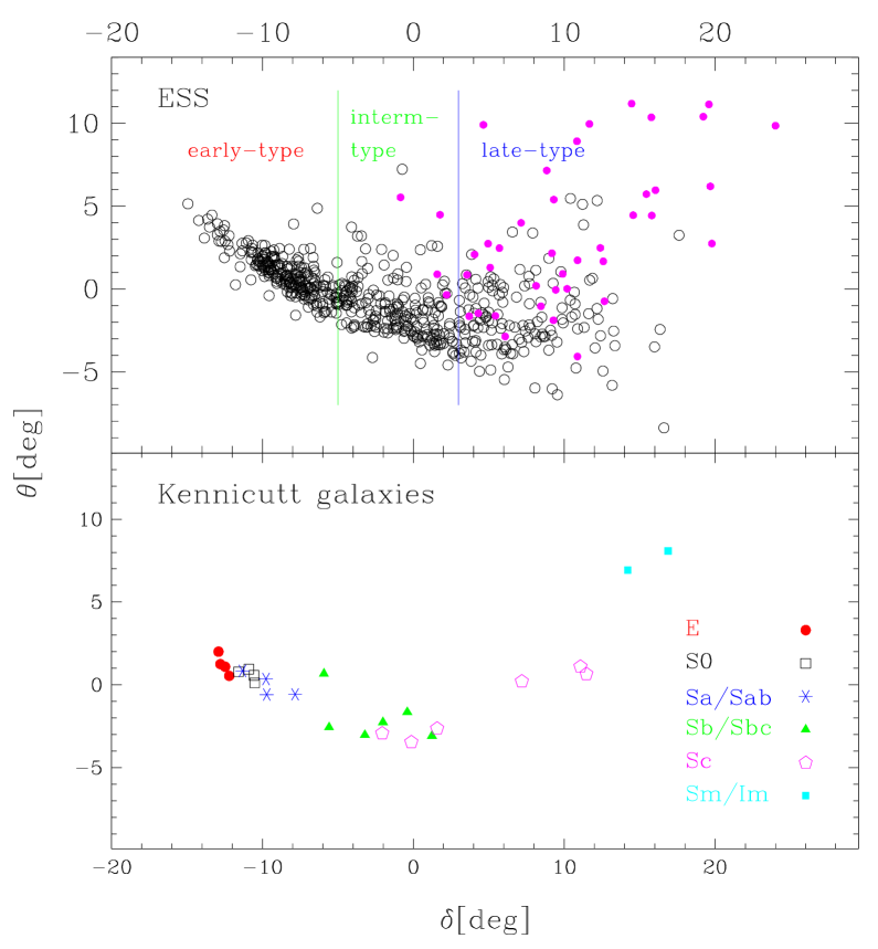
Figure 2: a) Top panel: spectral classification parameters $\delta$ and $\theta$ for the 603 ESO-Sculptor spectra with $R_{\mathrm{c}}\leq 20.5$ and a PCA defined spectral class $\delta_{1}-\theta_{1}$ (see Sect. 2.2 for details). Spectra are getting bluer toward larger values of $\delta$. Galaxies with EW[OII] $<$ 30 Å  are shown as black open circles, those with EW[OII] $\geq$ 30 Å as magenta filled circles. The vertical lines at $\delta=-5$ and $\delta=3$ indicate the limits between the 3 spectral classes used for the calculation of the luminosity functions (see Sect. 2.5). b) Bottom panel: $\delta$ and $\theta$ parameters obtained by projection of 26 Kennicutt spectra Kennicutt (1992) onto the ESS PCs used in a). To correct for the systematic color shift in the ESS spectra, a constant offset of $-2.5^{\circ}$ is applied to the $\delta$ values for the Kennicutt spectra (see Sect. 2.4). The morphological types for the Kennicutt galaxies provides indications on the type content of the ESS spectral classes.

The classification plane shown in Fig. 2a is obtained by restricting the spectra to the rest-wavelength interval 3700–5250 Å (a common wavelength interval must be used for application of the PCA presented in Galaz & de Lapparent 1998), which is denoted $\delta_{1}-\theta_{1}$. For the ESS spectra, this wavelength interval provides the best compromise between having a large sample, and having a large wavelength coverage which includes a sufficient number of significant absorption and emission lines ([OII]$\lambda 3727$, [OIII]$\lambda$5007, Ca H&K $\lambda 3934$, 3968 and Mgb $\lambda 5175$). Among the ESS spectra, 728 galaxies (511 with $R_{\mathrm{c}}\leq 20.5$) have spectra which do cover the primary wavelength interval 3700–5250 Å. Most of the remaining galaxies can be classified using 2 secondary wavelength ranges: 97 galaxies (50 with $R_{\mathrm{c}}\leq 20.5$) have spectra covering only the 3700–4500 Å interval, and 47 galaxies (42 with $R_{\mathrm{c}}\leq 20.5$), the 4500–6000 Å interval. We therefore perform 2 additional PCAs, each using the spectra defined in each of the 2 secondary intervals; these PCAs provide the $\delta_{2}-\theta_{2}$ and $\delta_{3}-\theta_{3}$ planes respectively.

Comparison of the $\delta-\theta$ sequences for spectra covering both the 3700–5250 Å primary interval and one of the 2 secondary intervals then allows us to project all ESS spectra with a PCA type onto the reference $\delta_{1}-\theta_{1}$ sequence. A total of 568 spectra (corresponding to 513 galaxies, as multiple spectra of individual galaxies are included) can be projected onto both the $\delta_{1}-\theta_{1}$ and the $\delta_{2}-\theta_{2}$ planes. Note that only spectra observed in spectro-photometric conditions (see Sect. 2.4) are used in this projection analysis, with no $R_{\mathrm{c}}$ limit. The derived conversion is a linear transformation

$$\delta_{1}=1.0027\delta_{2}-0.036,$$ (2)

close to identity. From the 375 spectra (corresponding to 345 galaxies) which can be projected onto both the $\delta_{1}-\theta_{1}$ and the $\delta_{3}-\theta_{3}$ planes, a third order polynomial transformation is derived:

$$\delta_{1}=0.0013\delta_{3}^{3}-0.088\delta_{3}^{2}+1.95\delta_{3}+1.68.$$ (3)

The residuals in the $\delta$ conversions resulting from the use of Eqs. 2 or 3 are comparable to the random uncertainties in the measurement of $\delta$ (see Eq. LABEL:sigma_delta_theta). The values of $\theta$ show no systematic change from the $\delta_{1}-\theta_{1}$ plane to either of the 2 secondary planes. We therefore use

$$\begin{array}[]{ll}\theta_{1}&=\theta_{2}\\ \theta_{1}&=\theta_{3}.\\ \end{array}$$ (4)

Eq. 2 is then used to convert $\delta_{2}$ into $\delta_{1}$ for the 97 galaxies which can only be projected onto the restricted 3700–4500 Å interval, and Eq. 3 is used to convert $\delta_{3}$ into $\delta_{1}$ for the 47 galaxies which can only be projected onto the restricted 4500–6000 Å interval.

We emphasize that the rest-frame wavelength interval of each observed spectrum is determined by (i) the position of the object on the multi-object mask used for that specific observation, and (ii) the redshift of the galaxy. The first constraint affects the rest-frame wavelength interval randomly, whereas the second causes a systematic effect. The 3 wavelength intervals used for application of the PCA and derivation of the spectral type are therefore systematically related to the redshift of the galaxies: high redshift galaxies tend to be only defined in the restricted secondary interval 3700–4500 Å, whereas low redshift galaxies tend to be preferentially defined in the other secondary interval, 4500–6000 Å. This effect can be measured quantitatively using the mean redshift of the galaxies in each sample: the galaxies defined in the primary wavelength interval have $<z>=0.303\pm 0.115$, those defined in the 2 secondary intervals 3700–4500 Å and 4500–6000 Å have $<z>=0.396\pm 0.134$ and $<z>=0.141\pm 0.082$ resp. (the r.m.s. dispersion among each considered sample is indicated). We show below (see Fig. 3) that despite the relation between rest-wavelength and redshift, conversion to a unique PCA sequence defined by $\delta_{1}$ is free from biases in redshift.

To the remaining 17 galaxies (15 with $R_{\mathrm{c}}\leq 20.5$) which have no PCA type, a spectral class in the $\delta_{1}-\theta_{1}$ plane is assigned based on the relation between $\delta_{1}-\theta_{1}$ and the ESS cross-correlation types. The cross-correlation types are determined by cross-correlating each ESS spectrum with 6 templates representing an E, S0, Sa, Sb, Sc, and Irr galaxy resp.; these were obtained by averaging over Kennicutt spectra of the same morphological type (Kennicutt, 1992), after discarding MK270, an untypical S0 galaxy with strong emission lines (a total of 26 Kennicutt spectra, listed in Table 2 of Galaz & de Lapparent 1998, are used). Among the templates yielding a cross-correlation peak at the redshift of the object, the cross-correlation type is defined as the morphological type of the template yielding the highest correlation coefficient (see Bellanger et al., 1995). Using the ESS galaxies with both a PCA type in the $\delta_{1}-\theta_{1}$ plane and a cross-correlation type, we calculate the median and dispersion of $\delta_{1}$ and $\theta_{1}$ for each of the 6 cross-correlations types. Each of the 17 galaxies without PCA type is then assigned (i) a randomly drawn value of $\delta_{1}$ using a Gaussian probability distribution with the mean and r.m.s. dispersion measured for the corresponding cross-correlation type, and (ii) the mean value of $\theta_{1}$ for that cross-correlation type.

Application of the various transformations described above provides for each of the 889 galaxies with redshift (617 with $R_{\mathrm{c}}\leq 20.5$) a PCA classification onto the common $\delta_{1}-\theta_{1}$ plane. Figure 3 shows the type parameter $\delta_{1}$ as a function of redshift for all ESS galaxies with $R_{\mathrm{c}}\leq 20.5$. The full redshift range is represented at all spectral types $\delta$, suggesting the absence of any obvious bias related to redshift. Note that the major density variations along the redshift axis are due to large-scale clustering along the line-of-sight (some higher order variations with $\delta$, interpreted as segregation effects, are described in de Lapparent & et al. 2003b). Figure 3 thus confirms that the conversion to a unique spectral sequence $\delta_{1}$ using the transformations in Eqs. 2 and 3 above has been successful.

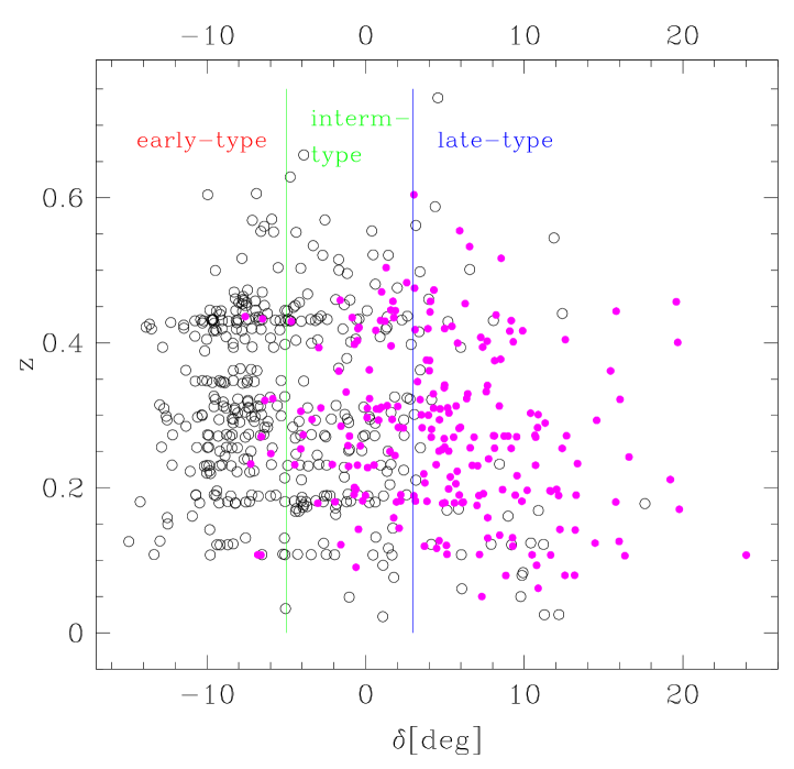
Figure 3: Spectral classification parameter $\delta$ as a function of redshift for the ESO-Sculptor galaxies with $R_{\mathrm{c}}\leq 20.5$. Galaxies with EW[OII] $<$ 10 Å  are shown as black open circles, those with EW[OII] $\geq$ 10 Å as magenta filled circles. The vertical lines at $\delta=-5^{\circ}$ and $\delta=3^{\circ}$ indicate the limits between the 3 spectral classes used for the calculation of the luminosity functions (see Sect. 2.5).

Figure 3 also shows that the various spectral types $\delta$ are represented at all redshifts. The defined early-type, intermediate-type and late-type spectral classes used for derivation of the LFs below, can therefore be used for examining the variations of the ESS galaxy populations with redshift (see de Lapparent et al., 2003). Moreover, Fig. 3 shows that galaxies with a significant equivalent width in the [OII]$\lambda$3727 emission line, defined as EW[OII] $\geq$ 10 Å, have preferentially later spectral type $\delta$, and that this relationship is homogeneous with redshift. This illustrates the absence of another kind of possible bias: the preferential selection of emission-line galaxies at the high redshift end of the ESS. This demonstrates that the adjustment of the spectroscopic exposure times for the ESS was successful in insuring that the absorption-line galaxies at the high redshift-end of the survey have spectra with sufficient signal-to-noise ratio for redshift measurement.

We also use Fig. 3 to justify that we do not report nor discuss the ESS LFs which would be derived from sub-samples based on the strength of the emission lines. As shown in Fig. 3, the fraction ESS galaxies with EW[OII] $\geq$ 10 Å is $3.9$% in the early-type class, $32.3$% in the intermediate-class, and $\sim 80.3$% in the late-type class (for the $R_{\mathrm{c}}\leq 20.5$ sample). The ESS LFs for the quiescent and star-forming galaxies are therefore expected to closely resemble the LFs for the early-type and late-type galaxies resp., and therefore would not provide any additional information over that based on the spectral-type LFs described in the subsequent Sects.

2.3 K-corrections

Calculation of the absolute magnitudes necessary for derivation of the galaxy LF requires knowledge of the K-corrections. Historically, K-corrections have been computed as a function of redshift and morphological type (Oke & Sandage, 1968; Pence, 1976; Loveday et al., 1992), the latter being based on visual classification. However, it was shown that the morphological type is strongly dependent on the expert who performs the classification (Lahav et al., 1995). Galaxy classification is also dependent on the central wavelength of the filter through which the galaxy is observed (Kuchinski et al., 2001), and on the image quality (van den Bergh et al., 2001); both are in turn dependent on redshift, and the latter also depends on seeing. Because K-corrections measure the change in flux in a given filter caused by the redshifting of the spectral energy distribution, a more direct and reliable approach for computing K-corrections is the use of spectral types, instead of morphological types.

Here, we use the ESS PCA spectral classification to calculate 2-dimensional K-corrections as a continuous function $K(z,\delta)$ of the spectral type $\delta$ and the redshift $z$. These in turn provide absolute $B$, $V$, and $R_{\mathrm{c}}$ magnitudes for the ESS galaxies. Note that the absolute magnitudes cannot be calculated directly from the observed spectra because: (i) their spectro-photometric accuracy ($\sim 7-10\%$) is insufficient, and $\sim 30\%$ of the spectra have a signal-to-noise ratio below 10; (ii) the rest-wavelength intervals covered by the $B$, $V$, and $R_{\mathrm{c}}$ filters are not always included in the observed spectra, as it depends on the combination of redshift and position of objects in the multi-object-spectroscopy mask. As a more robust and precise alternative, we determine the K-corrections from the spectrophotometric model of galaxy evolution PEGASE (Fioc & Rocca-Volmerange, 1997). The model spectra extend from 2000 Å to 10000 Å, thus allowing us to derive K-corrections in the $B$, $V$, and $R_{\mathrm{c}}$ bands up to $z\simeq 1.0$.

The PEGASE model allows one to generate a set of solar metallicity spectra with different ages, stellar formation rates (SFR) and initial mass functions (IMF). Although this feature is proposed in PEGASE, we do not include in the model spectra any nebular emission line, because line ratios depend on complex astrophysical conditions (gas densities, temperatures, etc.) which are not intended to be explored in full extent in the present analysis. Moreover, inclusion of the emission lines only change the derived K-corrections by $\sim 2\%$ in the most extreme emission-line galaxies. We have generated a large set of mock spectra in the wavelength interval $2000-10000$ Å using a Scalo IMF (Scalo, 1986), and a SFR of the form $\nu G_{F}$, where $\nu$ is a constant and $G_{F}$ the fraction of stellar ejecta available for further star formation. The adopted values of $\nu$ run from $\nu=0.02\times 10^{-3}$M_☉Myr^-1 to $\nu=10.0\times 10^{-3}$M_☉Myr^-1, with a typical step of $0.02\times 10^{-3}$M_☉Myr^-1, and the ages of the spectra vary from 0.01 Myr to 19.0 Gyr. In order to simplify, we assume that $G_{F}=1.0$ (other values do not change significantly the K-corrections). The resulting set of templates amounts to 438 mock spectra.

For specific derivation of the K-corrections, a PCA of the ESS data is performed using the observed spectra cleaned from their nebular emission lines. The $\delta-\theta$ sequence shown in top panel of Fig. 2 flattens to a $\delta^{\prime}-\theta^{\prime}$ sequence in which $\theta^{\prime}\sim 0^{\circ}\pm 2^{\circ}$ as this parameter measures the relative strength of the emission-lines; the values of $\delta^{\prime}$, the classifying parameter, show no systematic change: $<\delta-\delta^{\prime}>=1.14^{\circ}\pm 1.3^{\circ}$ (in both cases, the quoted uncertainty is the r.m.s. dispersion). This analysis provides the observed PCs, onto which the PEGASE templates described above are projected, after normalization by their scalar norm (see Galaz & de Lapparent, 1998); a spectral type $\delta^{\prime}$ is thus derived for all templates. Each template is then redshifted to all redshifts between $z=0$ to $z=1.0$ using increments $\Delta z=0.05$. We finally compute for each of the Johnson $B$, $V$ and the Cousins $R_{\mathrm{c}}$ bands, the K-corrections for the mock spectrum $j$ with a spectral type $\delta^{\prime}$ and redshift $z$ as $K_{j}=K_{j}(z,\delta^{\prime})$ using the K-correction definition (Oke & Sandage, 1968):

$$K_{j}(z,\delta^{\prime})= 2.5\log(1+z)$$ (5)

$$+2.5\log\left(\frac{\int_{0}^{\infty}f_{j}(\lambda)S_{j}(\lambda)d\lambda}{\int_{0}^{\infty}f_{j}(\frac{\lambda}{1+z})S_{j}(\lambda)d\lambda}\right),$$

where $K_{j}(z,\delta^{\prime})$ is expressed in magnitudes, $f_{j}(\lambda)$ is the flux of spectrum $j$ at wavelength $\lambda$, and $S_{j}(\lambda)$ is the response curve of the standard filter (see Arnouts et al., 1997). For each filter, the $K_{j}(z,\delta^{\prime})$ are then fitted by a 2-D polynomial of degree 3 in $\delta^{\prime}$ and 4 in $z$, with the constraint that $K_{j}(z=0,\delta^{\prime})=0$. The derived analytical function $K(z,\delta^{\prime})$ allows us to compute for each observed spectrum its K-correction in each bandpass, using only its $\delta^{\prime}$ value and its redshift.

Note that we have not included in the K-correction any evolutionary correction, corresponding to the possible change of the spectrum during the interval of time elapsed between the moment of light emission and the present time. The evolutionary correction would correct the absolute magnitude to what would be observed at the present time. This is however related to the formation age of the objects, and is strongly model-dependent. The K-corrections derived here only account for the redshift effect of the spectra, and provide the absolute magnitudes of the objects at the time of emission (as is used in most observational analyses).

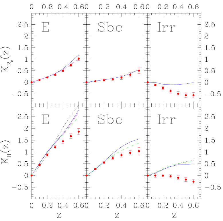
Figure 4: K-corrections obtained from the PEGASE templates (Fioc & Rocca-Volmerange, 1997, red filled circles with error-bars) in the $R_{\mathrm{c}}$ and $B$ band, compared with the K-corrections from Coleman et al. (1980, blue solid lines), Kinney et al. (1996, black dotted lines), Pence (1976, green short-dashed lines), and Poggianti (1997, magenta long-dashed line); for the $B$ K-corrections by Kinney et al. (1996), the K-corrections for type SB4 are used in panel “Irr”.

In Fig. 4, we show the $B$ and $R_{\mathrm{c}}$ K-corrections for the PEGASE templates, obtained as described above, and we compare them with those obtained by other authors from observed spectra (Pence, 1976; Coleman et al., 1980; Kinney et al., 1996) and other spectrophotometric models (Poggianti, 1997). The three ESS spectral types included in Fig. 4 (E, Sbc and Irr) are computed as follows: E type is defined by $\delta^{\prime}\leq-5.0^{\circ}$, Sbc by $-1.0^{\circ}\leq\delta^{\prime}\leq 5.0^{\circ}$, and Irr by $\delta^{\prime}\geq 10.0^{\circ}$ (see Fig. 2a); each point in Fig. 4 represents an average K-correction at a given redshift, and the error-bars represent the r.m.s. dispersion in the given $\delta^{\prime}$ intervals. Figure 4 shows that K-corrections for our templates agree well with the other measures in the $R_{\mathrm{c}}$ band (and in the $V$ band, not included in the graph), but they tend to be smaller in the $B$ band. In other words, our PEGASE templates are bluer at short wavelengths ($\lambda\la 4200$Å) than the spectra from which the K-corrections of Pence (1976), Coleman et al. (1980), Kinney et al. (1996), and Poggianti (1997) are derived. Moreover, the ESS K-corrections for type Irr tend to be bluer than those from the other authors in all bands; note that there exists few sources of K-corrections for Irr types, and most of them are based on the results of Pence (1976). We emphasize that in Fig. 4, we assume a correspondence between the PCA spectral types for the PEGASE templates and the Hubble morphological types used for the other measures mentioned. This correspondence may however not be optimal, which could explain part of the differences. For example, using $\delta^{\prime}\geq 3.0^{\circ}$ for defining Irr galaxies in the ESS (corresponding to the “late-type” class described in Sect. 2.5) eliminates the discrepancy with the Irr types of Pence (1976) in the 3 bands.

We have also applied the above analysis to the GISSEL96 models (Charlot et al., 1996), using solar metallicity and an instantaneous burst of star formation. Because the GISSEL96 models have lower fluxes in the wavelength interval $2000-4000$Å compared with the PEGASE models, the resulting K-corrections in the $B$ band for all 3 types (E, Sbc, Irr), and for Irr type in the $V$ and $B$ bands are larger than the K-corrections derived from PEGASE (Galaz, 1997), thus providing intermediate values between the K-corrections derived from PEGASE and those from Pence (1976), Coleman et al. (1980), Kinney et al. (1996), and Poggianti (1997). Our choice of using PEGASE rather than GISSEL96 for estimating the ESS K-corrections is motivated by the fact that PEGASE models provide a larger sample of templates, which are not systematically based on an instantaneous burst. Note that using the GISSEL96 templates for deriving the ESS K-corrections would only affect the $B$ and $V$ LFs. However, the major results derived in this article are based on the LFs in the $R_{\mathrm{c}}$ band, which is the least affected by changes in the SFR via the K-corrections (note that in the $V$ band, and to a greater extent, in the $B$ band, the LFs are also biased by color incompleteness, see Sect. 3.2).

The K-corrections for the ESS spectra are then calculated according to the redshift $z$ and spectral type $\delta^{\prime}$ of each galaxy. Here, we do not need to use a single spectral type scale for the whole sample, as designed in Sect. 2.2 (see Eqs. 2–3), which would introduce additional dispersion. The PEGASE templates are projected onto the 3 sets of PCs obtained with the spectra defined in the 3 wavelength ranges: the primary interval 3700–5250 Å, and the 2 secondary intervals 3700–4500 Å  and 4500–6000 Å; the corresponding spectral classification parameters $\delta_{1}^{\prime}$, $\delta_{2}^{\prime}$, and $\delta_{3}^{\prime}$ are derived. The polynomial fits $K_{i}(z,\delta_{i}^{\prime})$ are calculated for the 3 sets of PCs and spectral type sequences $\delta_{i}^{\prime}$ ($i=1,2,3$). Then, for each ESS spectrum, we use its spectral type $\delta_{i}^{\prime}$ and the corresponding polynomial function $K_{i}(z,\delta_{i}^{\prime})$ to calculate its K-correction (with $i$ defined by the wavelength range of the rest-frame spectrum). The absolute magnitude $M$ can subsequently be derived from the apparent magnitude $m$ and the redshift $z$ using

$$M=m-5\log d_{\mathrm{L}}(z)-K(z,\delta^{\prime})-25,$$ (6)

where

$$d_{\mathrm{L}}(z)=\frac{c}{H_{0}\;q_{0}^{2}}\left[zq_{0}+(q_{0}-1)(\sqrt{1+2q_{0}z}-1)\right]$$ (7)

is the luminosity distance in Mpc (Weinberg, 1976). Throughout the article, we use $H_{0}=100h$ km s^-1 Mpc^-1 for the Hubble constant, and $q_{0}=0.5$ (for $\Omega_{m}=1.0$ and $\Omega_{\Lambda}=0.0$).

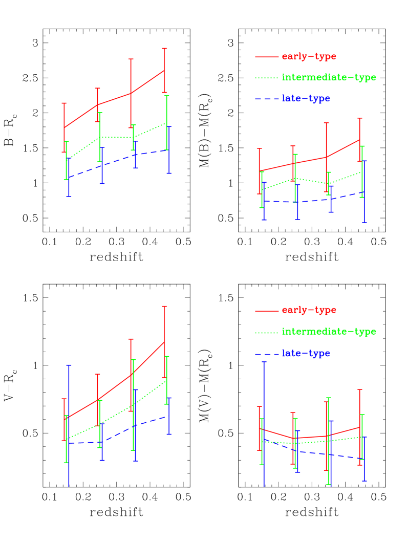
Figure 5: The mean absolute and apparent colors for galaxies with $R_{\mathrm{c}}\leq 20.5$ in each of the 3 ESO-Sculptor spectral classes used for calculation of the LFs, and in the 4 redshifts intervals bounded by 0.1, 0.2, 0.3, 0.4, and 0.5; red solid, green dotted, blue dashed lines connect the points for the early, intermediate, and late-type classes respectively. The left panels show the apparent colors and the right panels the absolute colors. The upper panels show the $B-R_{\mathrm{c}}$ colors, and the lower panels, the $V-R_{\mathrm{c}}$ colors. The error bars indicate the r.m.s. dispersion measured in the corresponding redshift interval. For clarity, the points for early and late-type galaxies are offset along the redshift axis by $-0.007$ and $0.007$, respectively.

Figure 5 provides indirect evidence that the PEGASE/PCA-based K-corrections yield adequate corrections of the ESS apparent magnitudes into absolute magnitudes. The left panels of Fig. 5 show the ESS $B-R_{\mathrm{c}}$ and $V-R_{\mathrm{c}}$ apparent colors. These show significant variations with redshift, as a result of the redshifting of the spectra. For the early-type galaxies, for which the effect is the largest, there is a $0.7^{\mathrm{mag}}$ reddening from $z=0.15$ to $z=0.45$. In contrast, the ESS $M(B)-M(R_{\mathrm{c}})$ and $M(V)-M(R_{\mathrm{c}})$ absolute colors, shown in the right panels of Fig. 5, display only small variations with redshift. The $0.3^{\mathrm{mag}}$ increase of $M(B)-M(R_{\mathrm{c}})$ for early-type galaxies between $z=0.15$ and $z=0.45$ might not be an intrinsic color effect, as the models of galaxy spectral evolution (Bruzual & Charlot, 1993; Fioc & Rocca-Volmerange, 1997) indicate little evolution in the interval $0\la z\la 0.5$. This increase could be caused by insufficient (i.e. too low) K-correction in the $B$ band, due to the relatively high flux of the PEGASE templates at wavelengths in the interval $2000-4000$Å (as discussed above; see also Fig. 4). The bluing of $M(V)-M(R_{\mathrm{c}})$ for the late-type galaxies by $0.15^{\mathrm{mag}}$ between $z=0.15$ and $z=0.45$ might be related to the strong evolution detected in this population (see de Lapparent et al., 2003). Overall, the residual variations in absolute colors with redshift are small, and confirm the reliability of the ESS K-corrections.

2.4 Random and systematic uncertainties in the ESS spectral sample

We now estimate the uncertainties in the ESS parameters used in this article for the calculation of the LFs: spectral type $\delta$, K-corrections, absolute magnitudes. The main source of error in the absolute magnitudes originate from the K-corrections. Once the spectral library is chosen (see Sect. 2.3), the K-corrections are essentially determined by the spectral classification, which in turn results from the errors in the flux calibration. Therefore, all mentioned parameters are dependent on the flux-calibration of the spectra, which we first examine.

The ESS spectra were flux-calibrated using spectro-photometric standards observed several times per observing night (see Galaz & de Lapparent, 1998). Among the 889 galaxies with a redshift measurement in the ESS spectroscopic sample (617 with $R_{\mathrm{c}}\leq 20.5$), 606 galaxies have at least 1 spectrum obtained in spectro-photometric conditions (402 with $R_{\mathrm{c}}\leq 20.5$); for the remaining 283 galaxies (215 with $R_{\mathrm{c}}\leq 20.5$), the single, 2 or 3 spectra of them were observed in either obvious non-spectro-photometric conditions or suspected as such. Among the 889 galaxies in the ESS spectroscopic sample, 204 of them have double spectroscopic measurements, and 35 have triple spectroscopic measurements. These multiple measurements provide 228 pairs of spectra with each a $\delta_{1}-\theta_{1}$ defined spectral type, which we use to assess our internal random errors. Among them, 102 pairs have both spectra taken in spectro-photometric observing conditions, and 126 pairs have at least one spectrum taken during a non-spectro-photometric night. The resulting r.m.s. dispersion in the spectral classification, and in the resulting K-corrections and absolute magnitudes is:

$$\begin{array}[]{ll}\sigma(\delta)&\simeq 2.5^{\circ}\;(2.8^{\circ})\\ \sigma(\theta)&\simeq 1.8^{\circ}\;(2.1^{\circ});\\ \end{array}$$ (8)

$$\begin{array}[]{ll}\sigma(K_{B})&\simeq 0.14\;\;{\rm mag}\;\;(0.21\;\;{\rm mag})\\ \sigma(K_{V})&\simeq 0.11\;\;{\rm mag}\;\;(0.14\;\;{\rm mag})\\ \sigma(K_{R_{\mathrm{c}}})&\simeq 0.07\;\;{\rm mag}\;\;(0.11\;\;{\rm mag});\\ \end{array}$$ (9)

$$\begin{array}[]{ll}\sigma(M_{B})&\simeq 0.16\;\;{\rm mag}\;\;(0.24\;\;{\rm mag})\\ \sigma(M_{V})&\simeq 0.13\;\;{\rm mag}\;\;(0.15\;\;{\rm mag})\\ \sigma(M_{R_{\mathrm{c}}})&\simeq 0.09\;\;{\rm mag}\;\;(0.12\;\;{\rm mag})\\ \end{array}$$ (10)

Note that in the present Sect., $\delta$ and $\theta$ stand for $\delta_{1}$ and $\theta_{1}$ resp., as described in Sect. 2.2. In Eqs. LABEL:sigma_delta_theta–LABEL:sigma_M, the first quoted dispersion is calculated from the 102 pairs of spectra observed in spectro-photometric conditions, whereas the value in parentheses indicates the dispersion calculated from the 126 pairs in which at least one spectrum was taken during a non-spectro-photometric night. The dispersion is calculated using a $2.5$-$\sigma$ rejection of the outliers.

We first note that adding in quadrature the $0.05^{\mathrm{mag}}$ uncertainties in the $B$ $V$ and $R_{\mathrm{c}}$ magnitudes (for $R_{\mathrm{c}}\la 21.0$; see Arnouts et al., 1997) to the values in Eq. LABEL:sigma_K yield values close to those in Eqs. LABEL:sigma_M. Second, as expected, the random errors are systematically larger for spectra which where taken in non spectro-photometric conditions. This sensitivity to the spectro-photometric observing conditions after the full sequence of data treatment performed to obtain absolute magnitude testifies on the quality of the ESS spectroscopic data-reduction, including the flux-calibration stage. A crude measure of the uncertainties in the flux calibration is obtained by calculating the r.m.s. deviation in the ratios of the spectra for each pair; the ratio of two spectra is measured as the ratio which most deviates from 1 in the wavelength interval $\sim 4000-9000$ Å. For the 102 pairs of spectro-photometric spectra, and for the 126 pairs with at least one non-spectrophotometric spectrum, the r.m.s. deviation in the ratios is $\sim 7-10$% and $\ga$ 10% respectively.

We also evaluate the contribution to the uncertainties in the absolute magnitudes caused by the errors in the redshifts. From the 228 pairs of independent spectra mentioned above, we measure an “external” r.m.s. uncertainty of $\sigma\sim 0.00055$ in the redshifts, which would correspond to an uncertainty of $\sim 165$ km/s in the recession velocity at small distances. From Eqs. 6 and 7, we measure that the contribution from the uncertainty in the redshift to the absolute magnitude is caused by the luminosity distance term $d_{L}$, with a contribution $\sigma(M|d_{L})\simeq 2.5\sigma(z)f(z)$, where $f(z)$ varies from $0.99$ at $z=0.1$ to $0.67$ at $z=0.5$. Therefore, the contribution to the total $\sigma(M)$ from the uncertainties in the redshifts is $\sigma(M|d_{L})\simeq 0.0009-0.0014$ for $0.1\leq z\leq 0.5$, which is negligeable compared with the values in Eq. LABEL:sigma_M.

A robust way to evaluate both the random and systematic uncertainties in the flux calibration for the ESS spectroscopic sample is to calculate “spectroscopic colors” by “observing” the spectra through the standard $B$, $V$, and $R_{\mathrm{c}}$ filters and compare them with the photometric colors. This procedure is only possible for a fraction of the spectra for which the appropriate wavelength range is available: $\sim 300$ spectra for which a $V-R_{\mathrm{c}}$ color can be calculated from the redshifted spectra (covering the $4800-8500$ Å interval), and another $\sim 300$ spectra for which a rest-frame $M_{B}-M_{V}$ color can be calculated from the rest-wavelength spectra (covering the $3600-6500$ Å interval). Because the spectroscopic colors are a function of the relative normalization of the filter transmission curves, these colors must be calibrated onto a sequence of standard stars. We use the spectra of the CTIO spectro-photometric standard stars which were originally obtained by Stone & Baldwin (1983) and Baldwin & Stone (1984), and were subsequently re-observed by Hamuy et al. (1992) and Hamuy et al. (1994). We also use the $B$ $V$ and $R_{\mathrm{c}}$ photometry provided by Landolt (1992) for these standard stars. The resulting calibrations are adjusted by linear regression and the dispersion in the $B-V$ and $V-R_{\mathrm{c}}$ color residual is in the range $0.005-0.015^{\mathrm{mag}}$ (which is negligeable compared with the 0.05 uncertainties in the ESS apparent magnitudes and to those in Eqs. LABEL:sigma_M).

“Spectroscopic colors” are then calculated from the ESS spectra, and the resulting mean offset between the photometric and spectroscopic colors and the dispersion around the mean are:

$$(V-R_{\mathrm{c}})_{\mathrm{spec}} -\,(V-R_{\mathrm{c}})_{\mathrm{phot}} =\,0.06\pm 0.23$$ (11)

$$(M_{B}-M_{V})_{\mathrm{spec}} -\,(M_{B}-M_{V})_{\mathrm{phot}} =\,0.10\pm 0.31$$ (12)

When the response curves for the standard filters are taken from other sources, they result in insignificant changes in Eqs. 11–12, thanks to the prior calibration of the spectroscopic colors with the CTIO standards. Removal of the atmospheric O₂ absorption bands from the spectra, near 6900 Å and 7600 Å, by linear interpolation from the surrounding continuum also yields insignificant changes in Eqs. 11–12.

We first consider the dispersion in the color offsets in Eqs. 11–12: 0.23 for $V-R_{\mathrm{c}}$ and $0.31$ for $M_{B}-M_{V}$. The r.m.s. uncertainties of $0.05^{\mathrm{mag}}$ in the $B$ $V$ and $R_{\mathrm{c}}$ magnitudes for $R_{\mathrm{c}}\la 21.0$ represent a negligeable contribution to these values. Part of dispersion in the color offsets calculated from apparent magnitudes (Eq. 11) originates from the random errors in the flux calibration. As mentioned above, these can contribute by $\ga 0.10$ to the dispersion in the spectroscopic magnitude, thus by $\ga 0.10\sqrt{2}\simeq 0.14$ to dispersion in the spectroscopic color $V-R_{\mathrm{c}}$. The $0.31^{\mathrm{mag}}$ dispersion in the color offset for absolute colors (Eq. 12) is larger than in Eq. 11 because it includes the dispersion in the K-corrections (Eq. LABEL:sigma_K).

We then examine the systematic offsets between the photometric and spectroscopic colors themselves, which can be interpreted as a magnitude scale offset. Because the r.m.s. dispersion in the color offsets given in Eqs. 11 and 12 is measured over the $\sim 300$ spectra considered in each case, the uncertainties in the scale offsets are obtained by dividing the dispersion values by $\sim\sqrt{300}$, which yields $0.013^{\mathrm{mag}}$ and $0.018^{\mathrm{mag}}$ respectively. These are negligeable compared with the $0.06$ and $0.10^{\mathrm{mag}}$ offsets in Eqs. 11 and 12, making these offsets highly significant. If we now assume that the mean scale offsets in Eqs. 11–12 originate from a systematic error in the flux-calibration, both offsets are consistent with the single interpretation that the ESS spectra have a 9% redder continuum every 1000 Å in the wavelength range $\sim 4000-8000$ Å. Because the effect is present in both the observed colors (Eq. 11) and the rest-frame colors (Eq. 12), the contribution from the ESS K-corrections to the color offset must be small – as these would only affect Eq. 12. We suggest that the systematic color offset is related to the shape of the transmission curves of the various CCDs used for the multi-object spectroscopic observations: the spectro-photometric calibrations may have under-corrected the lower sensitivity in the blue parts of the spectra, a common feature of CCD detectors.

Note that there may be a contribution to Eqs. 11–12 from aperture effects: the ESS spectra were obtained using long slits centered on the galaxies, which sample a larger fraction of the nuclei of galaxies as compared with their outer parts. Because color gradients are present in galaxies of varying types (Segalovitz, 1975; Boroson & Thompson, 1987; Vigroux et al., 1988; Balcells & Peletier, 1994), and in most cases correspond to several tenths of a magnitude bluer colors when going from the central to the outer regions of a galaxy, the spectroscopic colors may be biased towards redder colors. This effect is likely to contribute to both the systematic offset and the dispersion in the difference between the photometric and spectroscopic colors in Eqs. 11–12. Here, we cannot however separate the relative contributions of the intrinsic galaxy color gradients and of the instrumental response curve; this would require detailed simulations based on galaxy surface photometry.

Measurement of the (steep) slopes of the PCA classification parameter $\delta$ as a function of $(V-R_{\mathrm{c}})_{\mathrm{phot}}$ and $(M_{B}-M_{V})_{\mathrm{phot}}$ for the ESS spectra, allows us to convert the systematic offsets in Eqs. 11–12 into a systematic offset in the spectral type $\delta$. Both Eqs. 11 and 12 yield $\Delta\delta\simeq-2.5^{\circ}$, which contributes to validating our interpretation of the systematic color offsets in terms of a general flux-calibration error affecting all spectra over a wide wavelength range. Note that the derived systematic offset in $\delta$ is comparable in absolute value to the random error given in Eq. LABEL:sigma_delta_theta, and it is small compared with the wide range of $\delta$ covered by the galaxy types in the ESS, $-15^{\circ}\la\delta\la 20$ (see Fig. 2a). This offset has the net effect of shifting the ESS spectral sequence towards earlier-type spectra. It has the advantage of explaining the apparent systematic offset between the ESS spectra and the Kennicutt spectra in Fig. 8 of Galaz & de Lapparent (1998), the latter appearing shifted towards later-type spectra when projected onto the ESS PCA plane.

The above analysis of the systematic errors in the flux-calibration therefore indicates that when comparing the ESS $\delta$ spectral sequence with that for other samples, the values of $\delta$ for the comparison sample obtained by projection onto the ESS PCs should be offset by $-2.5^{\circ}$. If not, ESS galaxies would appear of earlier-type (too red) compared with other databases. This is used in the next Sect. where we compare the ESS spectral sequence with the Kennicutt spectra (1992), with the goal to make a correspondence between the ESS spectral type LFs and the intrinsic LFs per morphological class.

2.5 Sub-samples in spectral type

Although the full sequence of galaxy spectral types are present in the ESS (see Fig. 2a), the moderate number of objects in the survey limits the number of spectral classes which can be analyzed. We choose to separate the sample into 3 classes defined by $\delta\leq-5.0^{\circ}$, $-5.0^{\circ}\leq\delta\leq 3.0^{\circ}$ $3.0^{\circ}\leq\delta$; the corresponding galaxies are labeled “early-type”, “intermediate-type”, and “late-type” respectively. These values separate the ESS sample into 3 sub-samples with comparable numbers of objects in the $R_{\mathrm{c}}\leq 20.5$ sample ($\sim 200$ galaxies, see Table 2 below), and therefore allow us to measure the 3 LFs with comparable signal. The 3 samples are indicated in Fig. 2a by vertical lines.

Because the PCA spectral classification is continuous, the $\delta=-5.0^{\circ}$ and $\delta=3.0^{\circ}$ boundaries are arbitrary. A correspondence can nevertheless be made with the Hubble morphological classification by projecting Kennicutt spectra (Kennicutt, 1992) onto the ESS $\delta-\theta$ sequence: we use the 26 Kennicutt spectra listed in Table 2 of Galaz & de Lapparent (1998), discarding MK270, an untypical S0 galaxy with strong emission lines. As discussed in the previous Sect., this comparison requires that we offset the projections of the Kennicutt spectra onto the ESS PCs by $\Delta\delta=-2.5^{\circ}$. The resulting Kennicutt spectral sequence is plotted in Fig. 2b above, and confirms that the morphological types vary continuously along the Hubble sequence as $\delta$ increases, as already shown by Galaz & de Lapparent (1998).

Comparison of Figs. 2a and 2b suggest that the ESS early-type class contains predominantly E, S0 and Sa galaxies, the intermediate-type class, Sb and Sc galaxies, and the late-type class, Sc and Sm/Im galaxies. The chosen $\delta$ boundaries at $-5^{\circ}$ and $3^{\circ}$ therefore make physical sense as far as differentiating between intrinsically different LFs: they may help in separating the contributions from the bounded LFs for the Elliptical, Lenticular and Spiral galaxies, and the unbounded LF for the Irregular galaxies.

Figure 6: Spectral classification parameter $\delta$ as a function of absolute magnitude $M(R_{\mathrm{c}})$ for the ESO-Sculptor galaxies with $R_{\mathrm{c}}\leq 20.5$ sample. Galaxies with EW[OII] $<$ 10 Å  are shown as black open circles, those with EW[OII] $\geq$ 10 Å as magenta filled circles. The vertical lines at $\delta=-5^{\circ}$ and $\delta=3^{\circ}$ indicate the limits between the 3 spectral classes used for the calculation of the luminosity functions (see Sect. 2.5).

Figure 6 shows the ESS absolute magnitude $M(R_{\mathrm{c}})$ as a function of the spectral classification parameter $\delta_{1}$ for all galaxies with $R_{\mathrm{c}}\leq 20.5$. Here, there is a systematic correlation between spectral-type and luminosity of the galaxies, with a dimming by nearly $2.0^{\mathrm{mag}}$ from $\delta\simeq-10^{\circ}$ to $\delta\simeq 10^{\circ}$: this effect is a real property of the galaxies which causes the shift of $M^{*}$ towards fainter magnitudes for galaxies of later spectral type (Bromley et al. 1998; Madgwick et al. 2002; see also Sect. 3.2 below).

3 The shape of the ESS luminosity functions

3.1 Method

The ESS shows remarkable clustering in the galaxy distribution (Bellanger & de Lapparent, 1995). As far as the determination of the shape of the LF is concerned, simple methods such as the $1/V_{max}$ method (Schmidt, 1968) are strongly biased by the large-scale structures in the survey (Willmer, 1997). Instead, one must use statistical estimators based on ratios of number of galaxies, thus cancelling out the variations in density with distance. We also use maximum likelihood estimators which involve the probability that each galaxy in the survey is observed with its redshift and absolute magnitude. Two variants are used here: the step-wise maximum likelihood method (SWML hereafter) developed by Efstathiou et al. (1988), which does not assume any specific parameterization but requires to bin the data in steps of absolute magnitude; and the STY method (Sandage et al., 1979), which does not require to bin in magnitude intervals, but assumes a specific form for the LF. The SWML and STY solutions both account for the incompleteness per apparent magnitude interval according to the prescription by Zucca et al. (1994).

Because the ESS spectral-type LFs can be fitted by an exponential fall-off at bright magnitude and a power-law behavior at faint magnitudes, we use a Schechter (1976) parameterization for the STY fit (but see Sect. 4). This function is defined by 3 parameters, $\phi^{*}$ the amplitude, $L^{*}$ the “characteristic luminosity”, and $\alpha$ which determines the behavior at faint luminosities:

$$\phi(L)dL=\phi^{*}\left({L\over L^{*}}\right)^{\alpha}e^{-{L\over L^{*}}}d\left({L\over L^{*}}\right)$$ (13)

Rewritten in terms of absolute magnitude, Eq. 13 becomes:

$$\begin{array}[]{ll}\phi(M)dM&=0.4\ln 10\;\phi^{*}e^{-X}X^{\alpha+1}\;dM\\ {\rm with}&\\ X&\equiv{L\over L^{*}}=10^{\;0.4\,(M^{*}-M)}\\ \end{array}$$ (14)

where $M^{*}$ is the “characteristic magnitude”.

The performances of the SWML and STY techniques, and various other methods for deriving the LF have been tested on simulated samples by several authors (Willmer, 1997; Takeuchi et al., 2000). We refer the reader to these articles for discussion of the strengths and weaknesses of the SWML and STY methods. We did verified by application to various simulations matching the ESS configuration that these estimators are able to measure the input LF for an ESS-type survey, despite the large-scale spatial inhomogeneities (with the accuracy allowed by the number of galaxies in the sample). These simulations are mock ESS surveys with $\sim 240$, $\sim 2400$ and $\sim 24\,000$ points, and various types of large-scale inhomogeneities characterized by a modulation of the density in the redshift distribution (variations in density with position on the sky at constant redshift have no impact on the luminosity function). In all cases, the measured values of $M^{*}$, $\alpha$ and $\phi^{*}$ differ from the input values by the expected r.m.s. accuracy from the number of galaxies in the sample. We are therefore confident that the LFs measured here are unbiased by the ESS large-scale structure and other possible numerical effects.

Note that we have not incorporated into our STY fits the uncertainties in the absolute magnitudes: these can be accounted for by replacing the Schechter function by its convolved analog under the assumption of Gaussian errors in the magnitudes (with an r.m.s. dispersion denoted $\sigma_{\mathrm{M}}$ hereafter). Several analyses have been performed for evaluating the effect of the magnitude errors onto the Schechter parameters (Lin et al., 1996; Zucca et al., 1997; Ratcliffe et al., 1998). For $\sigma_{\mathrm{M}}=0.1^{\mathrm{mag}}$, Lin et al. (1996) find systematic offsets in the STY Schechter parameters of $\Delta M^{*}=+0.03^{\mathrm{mag}}$ and $\Delta\alpha=+0.03$, for nearly flat LFs with $\alpha\simeq-1$. Lin et al. (1997) then show that neglecting photometric errors with $\sigma_{\mathrm{M}}\leq 0.1^{\mathrm{mag}}$ only biases $M^{*}$ and $\alpha$ by at most $\Delta M^{*}=-0.02^{\mathrm{mag}}$ and $\Delta\alpha=-0.01$. For $\sigma_{\mathrm{M}}=0.2^{\mathrm{mag}}$, Zucca et al. (1997) measure $\Delta M^{*}=+0.10^{\mathrm{mag}}$ and $\Delta\alpha=+0.05$ for $\alpha$ in the range $-0.9$ to $-1.4$. For $\sigma_{\mathrm{M}}=0.22^{\mathrm{mag}}$, Ratcliffe et al. (1998) measure $\Delta M^{*}=+0.04^{\mathrm{mag}}$ and $\Delta\alpha=+0.10$ for an LF with $\alpha\simeq-1$. Based on these results, we expect that the random errors in the ESS absolute magnitudes, which are in the range $0.09^{\mathrm{mag}}\la\sigma_{\mathrm{M}}\la 0.24^{\mathrm{mag}}$ (Eq. LABEL:sigma_M), would yield systematic offsets $0.03^{\mathrm{mag}}\la\Delta M^{*}\la 0.10^{\mathrm{mag}}$ and $0.03\la\Delta\alpha\la 0.10$. The random errors in the Schechter parameters for the ESS LFs are in the range $0.15-0.30$ (see Table 2 below) and are thus larger than these systematic errors. We therefore neglect the uncertainties in the absolute magnitudes in the calculation of the STY solution.

3.2 The ESS luminosity functions per spectral type

Figure 7 plots the measured LFs for the 3 galaxy types in each filter, restricted to the nominal limits given in bold face in Table 1. The points represent the SWML solution, and the curves show the STY fit using a Schechter parameterization whose parameters $M^{*}$ and $\alpha$ are listed in Table 2. Figure 7 also shows the histograms of absolute magnitude, which allow one to evaluate how the ESS samples populate the measured LFs. Contrary to clusters of galaxies, where all galaxies occupy approximately the same volume, these histograms cannot be used as such, as galaxies with fainter magnitudes are detected in shallower samples.

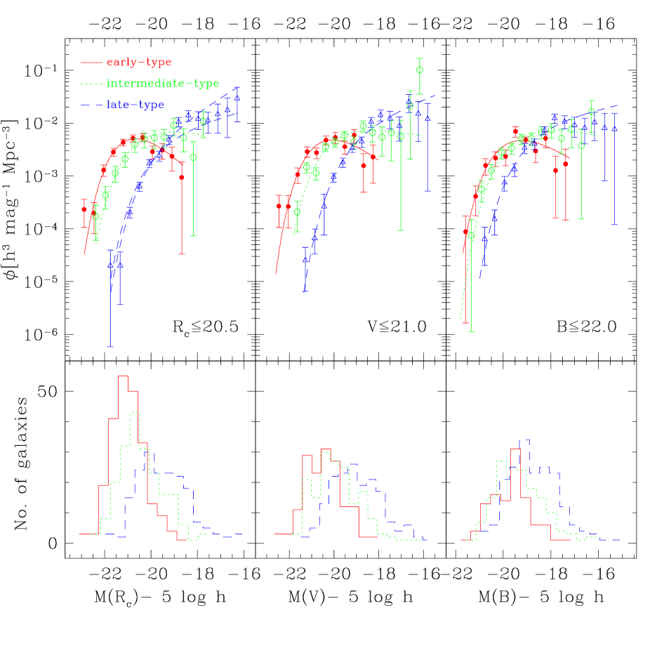
Figure 7: The ESO-Sculptor luminosity functions for the early-type, intermediate-type, and late-type galaxies at the nominal limits in the 3 filters: $R_{\mathrm{c}}\leq 20.5$, $V\leq 21.0$ and $B\leq 22.0$. Symbols indicate the SWML solution, and lines the STY solution: early-type are shown as red filled circles and red solid lines; intermediate-type as green open circles and green dotted lines; late-type as blue open triangles and blue dashed lines. The flatter curve for the late-type galaxies in the $R_{\mathrm{c}}\leq 20.5$ sample has $\alpha=-1.3$ (see text for details). The Schechter parameters of the STY solutions are listed in Tables 2 and 3. The amplitudes of the SWML points are adjusted by least-square fits to the STY solutions. The histograms show for each filter the number of galaxies used in the calculation of the corresponding LFs as a function of absolute magnitude (with the same line coding as for the STY solutions).

Table 2: Schechter parameters for the ESO-Sculptor luminosity functions, in the Cousins $R_{\mathrm{c}}$ and Johnson $V$ and $B$ filters.

early-type galaxies
Sample	$N$	$<\delta>$	$M^{*}-5\log h$	$\alpha$
(1)	(2)	(3)	(4)	(5)
$R_{\mathrm{c}}\leq 20.5$	232	-8.469	$-20.56\pm 0.14$	$+0.11\pm 0.23$
$R_{\mathrm{c}}\leq 21.0$	278	-8.385	$-20.61\pm 0.14$	$-0.02\pm 0.20$
$R_{\mathrm{c}}\leq 21.5$	291	-8.376	$-20.69\pm 0.14$	$-0.13\pm 0.17$
$V\leq 21.0$	156	-8.576	$-20.26\pm 0.18$	$-0.16\pm 0.24$
$V\leq 21.5$	210	-8.497	$-20.08\pm 0.14$	$+0.03\pm 0.22$
$V\leq 22.0$	266	-8.420	$-20.08\pm 0.15$	$-0.37\pm 0.21$
$V\leq 22.5$	285	-8.379	$-20.05\pm 0.15$	$-0.40\pm 0.20$
$B\leq 22.0$	108	-8.511	$-19.52\pm 0.24$	$-0.24\pm 0.33$
$B\leq 22.5$	150	-8.448	$-19.50\pm 0.22$	$-0.55\pm 0.29$
$B\leq 23.0$	204	-8.397	$-19.18\pm 0.21$	$-0.74\pm 0.31$
$B\leq 23.5$	240	-8.400	$-19.07\pm 0.22$	$-0.97\pm 0.30$
intermediate-type galaxies
Sample	$N$	$<\delta>$	$M^{*}-5\log h$	$\alpha$
$R_{\mathrm{c}}\leq 20.5$	204	-1.082	$-20.43\pm 0.17$	$-0.73\pm 0.19$
$R_{\mathrm{c}}\leq 21.0$	247	-0.995	$-20.63\pm 0.17$	$-0.80\pm 0.15$
$R_{\mathrm{c}}\leq 21.5$	270	-1.006	$-20.85\pm 0.19$	$-1.07\pm 0.13$
$V\leq 21.0$	169	-0.848	$-19.96\pm 0.18$	$-0.79\pm 0.19$
$V\leq 21.5$	216	-0.931	$-19.94\pm 0.14$	$-0.58\pm 0.17$
$V\leq 22.0$	249	-0.987	$-19.86\pm 0.12$	$-0.52\pm 0.15$
$V\leq 22.5$	266	-0.979	$-19.93\pm 0.12$	$-0.76\pm 0.14$
$B\leq 22.0$	154	-0.681	$-19.37\pm 0.20$	$-0.75\pm 0.21$
$B\leq 22.5$	193	-0.795	$-19.37\pm 0.17$	$-0.69\pm 0.18$
$B\leq 23.0$	225	-0.850	$-19.02\pm 0.15$	$-0.44\pm 0.19$
$B\leq 23.5$	242	-0.920	$-19.07\pm 0.16$	$-0.61\pm 0.17$
late-type galaxies
Sample	$N$	$<\delta>$	$M^{*}-5\log h$	$\alpha$
$R_{\mathrm{c}}\leq 20.5$	181	8.215	$-19.84\pm 0.24$	$-1.64\pm 0.23$
$R_{\mathrm{c}}\leq 21.0$	268	8.549	$-19.92\pm 0.19$	$-1.46\pm 0.18$
$R_{\mathrm{c}}\leq 21.5$	309	8.787	$-20.08\pm 0.21$	$-1.48\pm 0.16$
$V\leq 21.0$	168	8.393	$-19.34\pm 0.23$	$-1.42\pm 0.22$
$V\leq 21.5$	251	8.626	$-19.44\pm 0.17$	$-1.22\pm 0.17$
$V\leq 22.0$	293	8.653	$-19.41\pm 0.15$	$-0.93\pm 0.15$
$V\leq 22.5$	308	8.738	$-19.49\pm 0.14$	$-0.86\pm 0.14$
$B\leq 22.0$	190	8.670	$-19.00\pm 0.20$	$-1.25\pm 0.20$
$B\leq 22.5$	255	8.808	$-18.95\pm 0.17$	$-1.06\pm 0.17$
$B\leq 23.0$	279	8.825	$-19.00\pm 0.16$	$-0.80\pm 0.16$
$B\leq 23.5$	287	8.765	$-18.96\pm 0.15$	$-0.62\pm 0.14$

• Limiting magnitude.

• Number of galaxies in the sub-sample used for computation of the derived LF.

• Average spectral type $\delta$ for the sub-sample.

• Characteristic magnitude of the LF obtained by an STY Schechter fit (see Eq. 14).

• Slope at faint magnitudes of the LF obtained by an STY Schechter fit (see Eq. 14).

Table 3: Amplitude $\phi^{*}$ of the LFs in the Johnson $B$, $V$ and Cousins $R_{\mathrm{c}}$ bands for the 3 spectral classes in the ESO-Sculptor redshift survey.

Sample	early-type	intermediate-type	late-type
	$z\leq 0.55$	$z\leq 0.55$	$0.1\leq z\leq 0.2$
$R_{\mathrm{c}}\leq 20.5$	0.01477	0.01361	0.00652
$V\leq 21.0$	0.01392	0.01366	0.00848
$B\leq 22.0$	0.01336	0.01416	0.01013

• This table is extracted from Table 2 of de Lapparent et al. (2003), to be consulted for details. $\phi^{*}$ is in  $h^{3}$ Mpc^-3 mag^-1 .

Table 2 also lists the number of galaxies and average spectral type $<\delta>$ for each sub-sample for which we calculate a LF: the 3 spectral classes, in the 3 filters $B$ $V$ $R_{\mathrm{c}}$, to the nominal magnitude limits (see Table 1) and to fainter limits. Note that in the calculation of the LF, a K-correction is calculated for each galaxy using the individual values of $\delta^{\prime}$ and the calculated transformation $K(z,\delta^{\prime})$ described in Sect. 2.3 (Eq. 5); the average spectral types $<\delta>$ listed in Table 2 are thus only shown as indicative.

For the SWML points in Fig. 7, a bin size of $\Delta M=0.48^{\mathrm{mag}}$ is used in all 3 filters. Note that the SWML solution is weakly dependent on $\Delta M$ (Efstathiou et al., 1988), which we have checked using varying values of $\Delta M$ for the ESS LFs: smaller or larger bin sizes within a factor of 2 yield similar curves. For the STY solutions, we set the brightest and faintest limits to $-23.0$ and $-16.0$ resp. in $R_{\mathrm{c}}$, $-22.7$ and $-16.0$ resp. in $V$, $-21.6$ and $-15.0$ resp. in $B$; these bounds only exclude a couple of galaxies with anomalously bright or faint absolute magnitude. Because the amplitudes of both the STY and SWML solutions are undetermined, we adopt the following: we use for all STY curves in Fig. 7 the $\phi^{*}$ values listed in Table 3 (see de Lapparent et al. 2003 for details); then, for each sample, the SWML points are adjusted by least-square fit to the STY solutions. Because the amplitude $\phi^{*}$ strongly evolves with redshift for the late-type galaxies (see de Lapparent et al., 2003), Table 3 lists for that sample the average amplitude in the interval $0.1\leq z\leq 0.2$; in contrast, the integrated estimate of $\phi^{*}$ for $z\leq 0.55$ is used for the early-type and late-type samples (see de Lapparent et al., 2003).

Figure 7 shows that the ESS “general” LF is a composite function of at least 3 different galaxy populations: at bright magnitudes ($M[R_{\mathrm{c}}]\la-21$), early-type and intermediate-type galaxies dominate the population, whereas at the faint-end, they are outnumbered by the late-type galaxies, which show a steep increase in number density. The fact that these trends are observed in all 3 filters $B$ $V$ $R_{\mathrm{c}}$, suggests that differences in the LFs between the 3 spectral classes are not due to a color-dependent effect (such as star formation, for example), but rather reveal truly different mass distributions for the various galaxy types. Figure 8 shows the 1-$\sigma$ error ellipses for the LFs measured at $R_{\mathrm{c}}\leq 20.5$ in each of the 3 spectral classes: the error ellipses are well separated, and the slope $\alpha$ is significantly steeper at more than the 3-$\sigma$ level from one class to the next, when going from the early-type to the late-type galaxies.

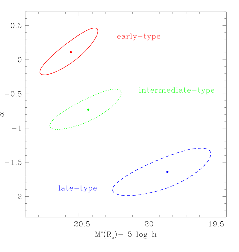
Figure 8: The best-fit parameters (filled circles) and the 1-$\sigma$ error ellipses for $M^{*}$ and $\alpha$ as derived from the STY fit of the LFs to $R_{\mathrm{c}}\leq 20.5$ for the 3 galaxy classes in the ESO-Sculptor Survey: early-type (red solid line); intermediate-type (green dotted line); late-type (blue dashed line).

We also show in Fig. 9, the distribution of absolute magnitude $M(R_{\mathrm{c}})$ versus redshift for the 3 ESS spectral classes. Although all spectral classes are detected at all redshifts in the ESS, as shown in Fig. 3, there is a strong correlation between absolute magnitude and redshift, due to the limit in apparent magnitude. Figure 9, shows that at the high redshift end of the ESS ($z\ga 0.4$), only galaxies brighter than $M_{R_{\mathrm{c}}}\simeq-20.0$ can be detected whereas faint galaxies (with $M(R_{\mathrm{c}})\ga-18.0$) can only be detected the low redshift end of the ESS ($z\la 0.15$). Only galaxies in the magnitude interval $-22.0\la M_{R_{\mathrm{c}}}\la-20.5$ can be observed in the full ESS redshift range $z\sim 0.1$ to $z\sim 0.5$. Figure 9 also shows that the small volume probed at $z\la 0.1$ tends to under-sample the number of galaxies at low levels of the LF: at $M(R_{\mathrm{c}})\la-20.0$ and $z\la 0.1$, no ESS galaxies of any class is detected, as the amplitude of all 3 LFs are below the minimal threshold for detecting at least one galaxy in the small sampled volume.

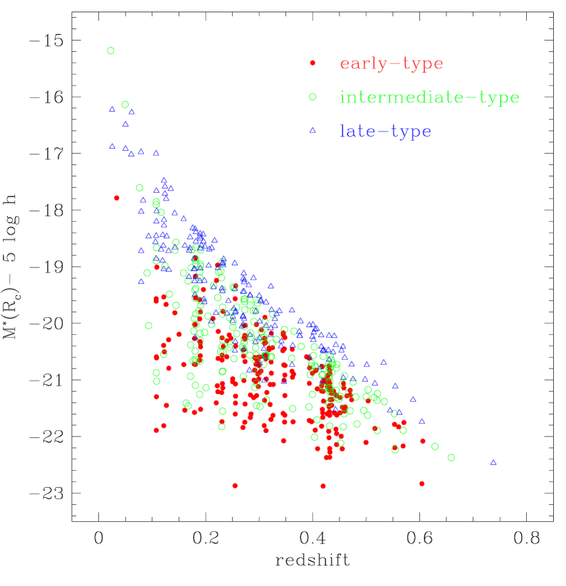
Figure 9: Absolute $R_{\mathrm{c}}$ magnitudes as a function of redshift $z$ for the ESO-Sculptor Survey galaxies with $R_{\mathrm{c}}\leq 20.5$. This graph shows how the limit in apparent magnitude biases the range of absolute magnitudes detected at increasing redshift, and how the varying K-corrections per spectral type affect the faintest absolute magnitude reached at a given redshift.

Note that the fainter absolute magnitudes probed by the ESS LF at a given redshift when going from early-type to late-type in Fig. 7 are also partly due to the decrease of K-corrections for later galaxy spectral types (see Fig. 4 and Eq. 6 in Sect. 2.3): the faint bound of the absolute magnitude distribution is a function of redshift and K-correction and is defined by replacing $m$ in Eq. 6 with the $R_{\mathrm{c}}=20.5$ apparent magnitude limit.

Table 2 shows that for the early-type galaxies, the slope $\alpha$ at the nominal magnitudes is in the range $-0.24$ to $0.11$ for the 3 filters, which results in a decrease in the number density of galaxies a faint magnitudes, whereas for the intermediate-type galaxies, $\alpha$ is close to the value $\alpha=-1$ for a flat slope, and remains nearly constant in all filters at the nominal magnitudes: $-0.76\leq\alpha\leq-0.75$. In contrast, the faint-end slope for the late-type galaxies is significantly steeper than for the early-type and intermediate-type galaxies, and varies at the nominal magnitudes from $-1.64$ in the $R_{\mathrm{c}}$ filter, to $-1.25$ in the $B$ filter. This corresponds to a steep increase in the number density of Sc+Sm/Im galaxies at faint magnitudes.

To estimate quantitatively whether the Schechter parameterization is a good description of each LF, we compare the SWML solution with the STY fits using the likelihood ratio defined by Efstathiou et al. (1988), which is distributed asymptotically like a $\chi^{2}$ probability distribution $P_{\phi}(\nu)$ with $\nu$ the number of degrees of freedom in the STY fit. To the nominal magnitude limits in the $R_{\mathrm{c}}$, $V$ and $B$ samples, the likelihood ratios are $0.81$, $0.83$ and $0.73$ resp. for the early-type LFs, $0.75$, $0.71$ and $0.52$ resp. for the intermediate-type LFs, and $0.46$, $0.44$ and $0.31$ resp. for the late-type LFs. The high values of the likelihood ratios for the early-type and intermediate-type classes indicate that the corresponding Schechter parameterizations are good representations of these LFs in the 3 photometric bands.

For the late-type galaxies, although the likelihood ratios of the STY solution remain within the range corresponding to an acceptable fit, they are systematically smaller than for the early-type and intermediate-type galaxies in each band. We interpret this effect as symptomatic of the difficulty to match both the intermediate magnitude range of the late-type LF ($-20\la M\la-18$ in $R_{\mathrm{c}}$ and $V$; $-19\la M\la-17$ in $B$) and the faint end ($M\ga-18.0$ in $R_{\mathrm{c}}$ and $V$; $M\ga-17$ in $B$) when using a Schechter parameterization. Figure 7 shows that the faintest 4 points of the SWML solution with $-18\la M\la-16$ in the $R_{\mathrm{c}}\leq 20.5$ late-type LF lie systematically below the STY fits. The same effect is observed in the $B$ band, but could be partly due to incompleteness (see Sect. 3.3 below); we then restrict the discussion to the $R_{\mathrm{c}}$ late-type LF. Because of the inherent under-sampling of the faint-end of the LF (see above), the faintest 4 magnitude bins in the late-type SWML solution contain 5 or less galaxies each, and thus poorly constrain the STY fit. The steep faint-end slope $\alpha=-1.64\pm 0.23$ is therefore determined by the 93 galaxies in the interval $-20.0\la M(R_{\mathrm{c}})\la-18.0$. Ideally, the faint end slope $\alpha$ should be determined by the faint end points of the SWML solution. We also plot in Fig. 7 the late-type STY solution with $\alpha=-1.3$, which corresponds to the flattest slope allowed by the STY fit at the 1-$\sigma$ level (see Fig. 8). Whereas $\alpha=-1.3$ better matches the 4 faint-end points of the late-type LF, it lies systematically below the SWML points in the brighter interval $-19\la M(R_{\mathrm{c}})\la-18$. A similar effect is observed for the late-type LF obtained from the fainter sample $R_{\mathrm{c}}\leq 21.5$: this sample contains 128 additional galaxies, and yields a steep slope for the STY fit $\alpha=-1.48\pm 0.16$ (see Table 2) which is determined by 169 galaxies with $-20.0\la M(R_{\mathrm{c}})\la-18.0$ and provides a good visual match to the SWML points in this interval; the faintest 3 points of the SWML solution (with $M(R_{\mathrm{c}})\ga-17.5$) however lie systematically below the STY solution. This illustrates the difficulty to fit the ESS late-type LFs using a single Schechter function. In Sect. 4.5 we show that a two-component function (Gaussian + Schechter) provides a better adjustment.

Figure 7 also indicates that the bright magnitude fall-off of the $V$ and $R_{\mathrm{c}}$ LFs for the late-type galaxies is fainter than for the early-type and intermediate-type galaxies by more than $1^{\mathrm{mag}}$. The smaller offset of the LF bright-end fall-off in the $B$ band can be interpreted as follows. At the median redshift $z\sim 0.3$ of the ESS, the portions of the galaxy spectra shifted into the $R_{\mathrm{c}}$ and $V$ filter correspond approximately to the $V$ and $B$ region resp. in rest-wavelength. The measured LFs thus detect the optical parts of the rest-wavelength spectral energy distribution. In contrast, at $z\sim 0.3$, the observed $B$ band probes the rest-frame spectral energy distribution in the near UV, which is highly sensitive to star formation; because the late-type galaxies have higher star formation than the earlier types, they appear relatively brighter in the $B$ band as compared with the $R_{\mathrm{c}}$ and $V$ bands.

Note that in a Schechter parameterization, offsets in the bright-end fall-off of the LF are poorly measured by the differences in $M^{*}$. In Fig. 7, the magnitude shift between the bright-ends for the early and late-type LFs is $\sim 1.7^{\mathrm{mag}}$ for the $R_{\mathrm{c}}\leq 20.5$ sample, $\sim 1.5^{\mathrm{mag}}$ for the $V\leq 21.0$ sample, and $\sim 1.0^{\mathrm{mag}}$ for the $B\leq 22.0$ sample (we measure it at $\phi\simeq 10^{-3}$ $h^{3}$ Mpc^-3 mag^-1). In contrast, the difference in $M^{*}$ between the early and late-type LF is $0.72$ mag, $0.92$ mag, and $0.52^{\mathrm{mag}}$ for the $R_{\mathrm{c}}\leq 20.5$, $V\leq 21.0$, and $B\leq 22.0$ LFs respectively (see Table 2). This effect is due to the strong correlation between the $M^{*}$ and $\alpha$ Schechter parameters (Schechter, 1976): for differing values of the slope $\alpha$, $M^{*}$ shifts to different parts of the LF and marks differently the fall-off of the bright-end. This indicates that in a comparison of Schechter LFs, the difference in $M^{*}$ must be increased by $0.5$ to $1.0^{\mathrm{mag}}$ to derive the shift in the bright-end between a LF with $\alpha\sim 0$ and a LF with $-1.6\la\alpha\la-1.2$. This effect is conveniently overcome by using Gaussian LFs for the giant galaxies, which have a well defined peak and r.m.s. dispersion (see Sect. 4).

3.3 Variations with filter and magnitude limit

Table 4: Comparison of the differences in the Schechter characteristic magnitudes and the mean absolute colors of the galaxies in the Johnson $B$, $V$ and Cousins $R_{\mathrm{c}}$ bands for the 3 spectral classes in the ESO-Sculptor redshift survey to $R_{\mathrm{c}}\leq 20.5$.

Spectral type	$M^{*}(B)-M^{*}(R_{\mathrm{c}})$	$<M(B)-M(R_{\mathrm{c}})>$	$M^{*}(V)-M^{*}(R_{\mathrm{c}})$	$<M(V)-M(R_{\mathrm{c}})>$
early-type	$1.04\pm 0.28$	$1.4\pm 0.4$	$0.30\pm 0.23$	$0.5\pm 0.2$
intermediate-type	$1.06\pm 0.25$	$1.0\pm 0.3$	$0.47\pm 0.25$	$0.4\pm 0.2$
late-type	$0.84\pm 0.31$	$0.8\pm 0.3$	$0.50\pm 0.33$	$0.4\pm 0.4$

We now discuss how the ESS LFs per spectral-type vary among the $R_{\mathrm{c}}$, $V$ and $B$ bands, and with magnitude limit. Table 4 lists the differences $M^{*}(B)-M^{*}(R_{\mathrm{c}})$ and $M^{*}(V)-M^{*}(R_{\mathrm{c}})$ obtained from the LFs parameters measured at the nominal magnitudes as a function of galaxy spectral type, and compares them with the mean absolute colors per spectral class for the galaxies with $R_{\mathrm{c}}\leq 20.5$, calculated as the mean difference between the absolute magnitudes in the 2 considered filters (see also left panels of Fig. 5, showing the variations in the absolute colors with redshift). Table 4 shows that for a given spectral type, the differences in the characteristic magnitudes $M^{*}$ from one filter to another simply reflect the mean absolute colors for the corresponding galaxy types.

As shown in Table 2, going to deeper magnitude limits than the nominal values increases the 3 spectral classes by a significant number of galaxies ($\sim$ 50–100 objects). For the $R_{\mathrm{c}}$ LF, when going to the fainter limits listed in Table 2, the STY solution remains remarkably stable, despite the increasing incompleteness of the spectroscopic samples: the STY fits have consistent $M^{*}$ and $\alpha$ values within less than 2-$\sigma$. This is evidence for robustness of the $R_{\mathrm{c}}$ LFs, as the number of early-type, intermediate-type and late-type galaxies increases by 25%, 32% and 71% respectively from the nominal limit to the faintest limit $R_{\mathrm{c}}\leq 21.5$ (the large increase in the number of late-type galaxies is caused by a strong evolution in this population, see de Lapparent et al. 2003). Note that the variations of the LFs with the $R_{\mathrm{c}}$ magnitude limit provides a good illustration of the correlation between the 2 shape coefficients of the Schechter parameterization: when going from $R_{\mathrm{c}}\leq 21.0$ to $R_{\mathrm{c}}\leq 21.5$, the extreme bright-end bin of the SWML solution shifts from 1 to 2 galaxies; despite the large error bars, this causes a brightening of $M^{*}$ by 0.2 magnitudes; to compensate and match the SWML points at other magnitudes, $\alpha$ becomes steeper by $\sim 0.35$.

In contrast, the $V$ and $B$ faint spectroscopic samples suffer color biases which affect the corresponding LFs. Because the completeness of the spectroscopic catalogue sharply drops to nearly $50$% at $R_{\mathrm{c}}\sim 21.5$, the $V$ and $B$ catalogue are biased in favor of red objects for galaxies at or fainter than the nominal limiting magnitudes $V\leq 21.0$ and $B\leq 22.0$: near these limits, the $V$ and $B$ spectroscopic catalogues are be deficient in galaxies with bluer colors than $B-R_{\mathrm{c}}\simeq 1.5$ and $V-R_{\mathrm{c}}\simeq 0.5$ respectively. We measure that the resulting reddening in the observed $B-R_{\mathrm{c}}$ and $V-R_{\mathrm{c}}$ colors beyond the nominal $V$ and $B$ limits varies from $\sim 0.15$ to $\sim 0.40^{\mathrm{mag}}$ depending on the color and class considered, with, as expected, a larger value for earlier-type galaxies and in the $B$ band. Because at fainter limiting magnitudes, one probes more distant objects which are therefore redder (due to the K-correction), betters estimates of the color biases are given by the absolute colors. Whereas the average $M(B)-M(R_{\mathrm{c}})$ colors change by at most $\sim\pm 0.13^{\mathrm{mag}}$ when going from $R_{\mathrm{c}}\leq 20.5$ to $20.5\leq R_{\mathrm{c}}\leq 21.5$ sample, for the 3 spectral classes, the colors become redder by $0.21-0.24^{\mathrm{mag}}$ for the early-type and intermediate-type galaxies, when going to fainter limiting magnitudes in $V$ and $B$ respectively. The effect is smaller for the late-type galaxies, with a reddening in $M(B)-M(R_{\mathrm{c}})$ of $0.05^{\mathrm{mag}}$ and $0.13^{\mathrm{mag}}$ in the fainter $V$ and $B$ samples respectively. The change in the $M(V)-M(R_{\mathrm{c}})$ color when going to fainter magnitudes than the nominal limits are in the range $-0.06$ to $0.06$ for the 3 filters and 3 spectral types.

Overall, these colors biases are likely to be responsible for the $0.45^{\mathrm{mag}}$ dimming of the $M^{*}(B)$ magnitude from the $B\leq 22.0$ to the $B\leq 23.5$ sample for the early-type galaxies; and for the flattening of $\alpha$ by $\sim 0.6$ with nearly constant $M^{*}$ at fainter $V$ and $B$ magnitudes for the late-type galaxies (the other variations, for intermediate-type galaxies in the $B$ filter, and for early-type and intermediate-type galaxies in the $V$ filter, are smaller and correspond to less that 1-$\sigma$ deviations). Moreover, it is likely that the color biases affecting the $V$ and $B$ samples cause the flatter slope $\alpha$ for the late-type $B$ and $V$ LFs as compared with that in $R_{\mathrm{c}}$: even at the nominal magnitudes in the $B$ and $V$, these samples are deficient in the blue galaxies which populate the fainter magnitudes for late-type galaxies.

3.4 Comparison with the CNOC2 survey

The only comparable survey to the ESS is the CNOC2 (for “Canadian Network for Observational Cosmology”) redshift survey (Lin et al., 1999): as the ESS, the CNOC2 survey is based on medium resolution spectroscopy from which redshifts and spectral types are measured. The ESS and the CNOC2 also are the only redshift surveys providing spectral-type LFs in the $R_{\mathrm{c}}$ band at $z\sim 0.5$. The CNOC2 covers $0.692$ deg² and is limited to $R_{\mathrm{c}}\leq 21.5$. At variance with the ESS, the CNOC2 spectral classification is obtained by least-square fit of the $UBVR_{\mathrm{c}}I_{\mathrm{c}}$ colors to those calculated from the galaxy spectral energy distributions linearly interpolated between the 4 templates of E, Sbc, Scd and Im galaxy types defined by Coleman et al. (1980); the “early”, “intermediate”, and “late” spectral classes are then defined as corresponding to the E, Sbc, and Scd+Im templates (see Lin et al., 1999). The CNOC2 intrinsic LFs are measured from 611 early-type, 517 intermediate-type, and 1012 late-type galaxies.

Both the CNOC2 and ESS detect evolutionary effects in their $R_{\mathrm{c}}$ LFs (Lin et al., 1999; de Lapparent et al., 2003). Here we only consider the following LFs: for the ESS, the “average” LFs for each spectral type obtained in Sect. 3.2, by calculating the LFs over the full redshift range of the survey (see Table 2); for the CNOC2, we use the listed values of $\alpha$, for which no evolution is detected, and the listed values of $M^{*}$ at $z=0.3$ by Lin et al. (1999), as it nearly corresponds to both the median redshift of the survey and the peak of the redshift distribution (see Fig. 6 of Lin et al., 1999; $z=0.3$ is also close the peak redshift for the ESS).

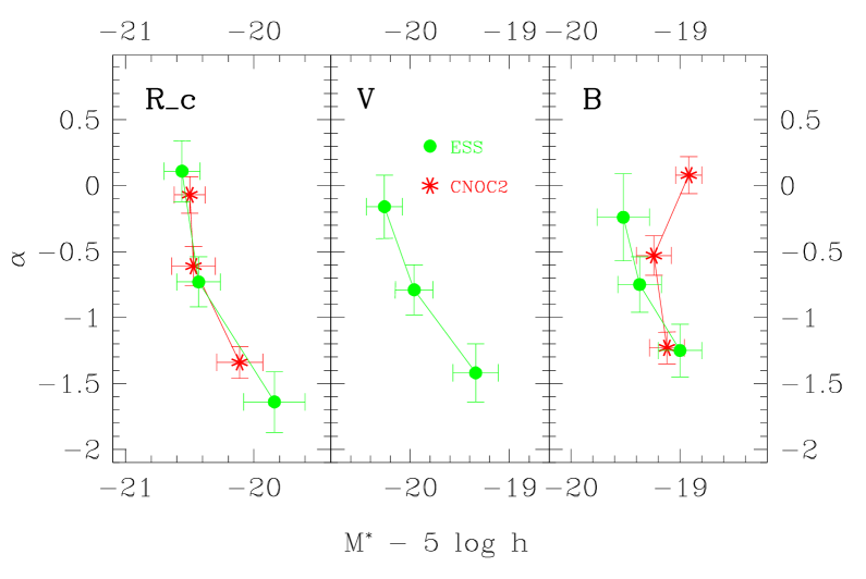
Figure 10: Comparison of the Schechter parameters $M^{*}$ and $\alpha$ for the ESO-Sculptor Survey in the $R_{\mathrm{c}}$, $V$, and $B$ bands with those from the CNOC2 (Lin et al., 1999). Galaxies of later spectral type are in the direction of steeper slopes $\alpha$.

Figure 10 plots the $M^{*}$ and $\alpha$ parameters for the ESS and the CNOC2 in the $R_{\mathrm{c}}$, $V$, and $B$ bands. The points for each survey are connected from one class to the next (red stars for the CNOC2, green filled circles for the ESS). Left panel of Fig. 10 shows that the values of $M^{*}$ and $\alpha$ for the CNOC2 $R_{\mathrm{c}}\leq 21.5$ sample are in close agreement with those for the ESS $R_{\mathrm{c}}\leq 20.5$ sample at the 1-$\sigma$ level. As in the ESS, the CNOC2 intrinsic LFs show a steepening in $\alpha$ and a dimming in $M^{*}(R_{\mathrm{c}})$ when going from early to late spectral types, with most of the dimming occurring between intermediate and late types. In the next Sect., we show that for the ESS, this dimming is a signature of the fainter magnitude late-type Spiral galaxies (Sc, Sm) detected in the late-type class, compared with the earlier Spiral types Sa and Sb included in the early and intermediate-type classes, respectively.

The agreement of the ESS and CNOC2 intrinsic LFs in the $R_{\mathrm{c}}$ band is a result of the similar morphological content of the spectral classes: the early, intermediate, and late-type classes contain predominantly E/S0, Sbc, and Scd/Im resp. in the CNOC2; in the ESS, they contain E/S0/Sa, Sb/Sc, and Sc/Sm/Im resp. (see Sect. 2.5). We further check the similar content of the ESS and CNOC2 by comparing the relative number of galaxies in each class. At $R_{\mathrm{c}}\leq 20.5$, the ESS early, intermediate and late-type class contain 38%, 33% and 29% of the galaxies, respectively. At $R_{\mathrm{c}}\leq 21.5$, the CNOC2 early, intermediate, and late-type classes contain 29%, 24%, and 47% of the galaxies, respectively. The 1-mag fainter limiting magnitude in the $R_{\mathrm{c}}$ band for the CNOC2, and the detected evolution in the amplitude of the late-type LFs in both the CNOC2 (Lin et al., 1999) and the ESS (de Lapparent et al., 2003), is likely to be responsible for the increase in the fraction of late-type galaxies in the CNOC2 compared with the ESS. For direct comparison with the CNOC2, we estimate the expected fraction of ESS galaxies per spectral class at $R_{\mathrm{c}}\leq 21.5$ as follows: in each of the 3 spectral classes lying in the 2 magnitude intervals $20.5<R_{\mathrm{c}}\leq 21.5$ and $20.5<R_{\mathrm{c}}\leq 21.5$, we correct the number of galaxies with a redshift measurement by the incompleteness in that magnitude interval (given in parenthesis in Table 1). This assumes that the incompleteness is independent of spectral class beyond the $R_{\mathrm{c}}\leq 20.5$ nominal limit, which is plausible as the observed galaxies beyond the nominal limit where chosen on the basis of total luminosity and crowding on the multi-object masks. The lower success rate in measuring redshifts for low signal-to-noise absorption-line spectra compared with emission-line spectra of similar signal-to-noise ratio might bias the galaxies with measured redshifts toward later spectral type; this is however a small effect, which we ignore here. The resulting estimated fractions of ESS galaxies per spectral class at $R_{\mathrm{c}}\leq 21.5$ are: 27%, 30%, and 43% for early, intermediate, and late-type respectively. The $\sqrt{N}$ uncertainties in the ESS and CNOC2 fractions are $1-2$% (taking into account 2-point clustering would slightly increase these uncertainties). The CNOC2 and ESS early-type classes therefore contain a consistent fraction of galaxies. In contrast, the CNOC2 intermediate-type class contains fewer galaxies than in the ESS, whereas the opposite is true for the late-type class. This suggests that the CNOC2 late-type class includes galaxies of earlier type than in the ESS late-type class. This might explain why the late-type LF for the CNOC2 has a flatter $\alpha$ and brighter $M^{*}$ than in the ESS (see Fig. 10).

There are 2 other surveys providing estimates of intrinsic LFs at $z\sim 0.5$ in a red filter: the sample of field galaxies extracted from the CNOC1 cluster survey (Lin et al., 1997), based on $gr$ photometry in the Thuan & Gunn (1976) system, in which the intrinsic LFs are derived from 2 color sub-samples; and the COMBO-17 survey (Wolf et al., 2003), based on the $r^{*}$ band (Fukugita et al., 1996), in which LFs are measured for 4 spectral classes. The results from these 2 surveys, and those from 3 other surveys at smaller redshifts (Lin et al., 1996; Brown et al., 2001; Nakamura et al., 2003) are analyzed in de Lapparent (2003), which provides an exhaustive comparison of all estimates of intrinsic LFs in the optical bands derived from surveys ranging from $z\simeq 0.03$ to $z\simeq 0.6$. The analysis of de Lapparent (2003) includes surveys in which the intrinsic LFs are based on either spectral classification, morphological type, rest-frame color, or strength of the emission-lines.

In the Johnson $V$ band, the ESS provides the first estimates of intrinsic LFs at $z\sim 0.3$. The corresponding Schechter parameters are plotted in the middle panel of Fig. 10, and show the similar dimming in $M^{*}$ and steepening in $\alpha$ for later types as detected in the $R_{\mathrm{c}}$ band. The only other existing measurements in the $V$ band are those provided by the Century Survey (Brown et al., 2001) based on 2 intervals of $V-R_{\mathrm{c}}$ rest-frame color; these are compared to the ESS in de Lapparent (2003).

Right panel of Fig. 10 shows the Schechter parameters for the ESS and CNOC2 LFs in the $B$ band. For the CNOC2, we have converted the listed values of $M^{*}(B_{\mathrm{AB}})$ for $z=0.3$ and $q_{0}=0.5$ into the Johnson $B$ band using $B-B_{\mathrm{AB}}=0.14$ (see Fukugita et al., 1995). The CNOC2 $B$ LFs are based on samples with nearly identical numbers of galaxies as in the $R_{\mathrm{c}}$ filter. The $B$ band intrinsic LFs for the 2 surveys also show the steepening in $\alpha$ from the early to the late-type classes. The agreement between the CNOC2 and ESS $B$ LFs is however not as good as in the $R_{\mathrm{c}}$ band, with a $\sim 2$-$\sigma$ difference between the $M^{*}$ values for the early-type LFs. This could be caused by the incompleteness of the ESS $B$ samples due to the $R_{\mathrm{c}}$ selection of the spectroscopic sample (see Sects. 2.1 and 3.3).

Several other redshift surveys provide estimates of $B$ LFs to $z\sim 0.5$: the Canada-France Redshift Survey (CFRS Lilly et al., 1995); the CNOC1 (Lin et al., 1997); the Norris survey (Small et al., 1997); the Autofib survey (Heyl et al., 1997); the CADIS (Fried et al., 2001); and the COMBO-17 survey (Wolf et al., 2003). We refer the reader to de Lapparent (2003), for comparison of the $B$ LFs among these surveys and with those measured at lower redshifts.

4 Composite adjustments of the ESS luminosity functions

In this section, we derive composite fits of the ESS luminosity functions per spectral-type by comparison with the LFs per morphological type measured from local groups and clusters (see Sect. 1). This analysis has the advantage of providing clues on the underlying morphological mix in the ESS spectral classes.

4.1 The local luminosity functions per morphological type

Comparing the local LFs to the ESS measurements requires to relate the extrapolated $B_{\mathrm{T}}$ magnitudes from the Third Reference Catalogue of Bright Galaxies (de Vaucouleurs et al., 1991) to the Johnson-Cousins system. To this end, we use the apparent photo-electric magnitudes in the Johnson $B$ band measured for Virgo cluster galaxies by Schroeder & Visvanathan (1996). The resulting $B_{\mathrm{T}}-B$ distribution as a function of morphological type has a bell shape with a large dispersion of $\sim 0.2^{\mathrm{mag}}$. We empirically adopt the values listed in column $M(B_{\mathrm{T}})-M(B)$ of Table 5, which lies within the $B_{\mathrm{T}}-B$ distribution and vary smoothly with morphological type (between $0.0$ and $0.3$, with a peak for type Sa). Note that although Schroeder & Visvanathan (1996) provide apparent colors, these are close to colors in absolute magnitudes at the small redshift of the Virgo cluster, hence the notation of absolute color in Table 5. We also list the Johnson-Cousins $B-V$ and $B-R_{\mathrm{c}}$ colors calculated by Fukugita et al. (1995) at redshift $z=0$, and deduce by combination with the $B_{\mathrm{T}}-B$ values the color transformation from $B_{\mathrm{T}}$ to the other ESS bands; these are also listed in Table 5 as absolute colors. For the ESS galaxies, derivation of the corresponding apparent colors would require use of the K-corrections described in Sect. 2.3.

Table 5: Color terms for converting absolute magnitudes from the $B_{\mathrm{T}}$ system into the Johnson-Cousins system used in the ESO-Sculptor survey.

Typea	$M(B_{\mathrm{T}})-M(B)$	$M(B)-M(V)$ b	$M(B_{\mathrm{T}})-M(V)$	$M(B)-M(R_{\mathrm{c}})$ b	$M(B_{\mathrm{T}})-M(R_{\mathrm{c}})$
E	0.10	0.96	1.06	1.57	1.67
S0	0.20	0.85	1.05	1.39	1.59
Sab	0.30	0.78	1.08	1.34	1.64
Sbc	0.20	0.57	0.77	1.09	1.29
Scd	0.10	0.50	0.60	1.00	1.10
Sm/Im	0.00	0.27	0.27	0.58	0.58
Spiral c	0.20	0.57	0.77	1.09	1.29

• Hubble morphological type.

• From Fukugita et al. (1995).

• The intermediate colors for type Sbc are used.

Table 6: Parameters of the Gaussian and Schechter LFs for the different morphological types, derived from local galaxy concentrations.

Morphological type	Type for	Gaussian $M_{0}-5\log h$				Gaussian $\Sigma$
	color term a	$B_{\mathrm{T}}$	$B$	$V$	$R_{\mathrm{c}}$
E	E	$18.33$ b	$-18.43$	$-19.39$	$-20.00$	$2.15\pm 0.36/1.32\pm 0.21$ b
S0	S0	$-18.90\pm 0.12$ b	$-19.10$	$-19.95$	$-20.49$	$1.13\pm 0.10$ b
Spiral	Sbc	$-18.20\pm 0.09$ b	$-18.40$	$-18.97$	$-19.49$	$1.37\pm 0.07$ b
Sa/Sb	Sab	$-19.6\pm 0.2$ c	$-19.9$	$-20.7$	$-21.2$	$0.9\pm 0.1$ c
Sc	Sbc	$-18.5\pm 0.2$ c	$-18.7$	$-19.3$	$-19.8$	$1.2\pm 0.1$ c
Sd/Sm	Scd	$-17.1\pm 0.2$ c	$-17.1$	$-17.4$	$-17.7$	$0.8\pm 0.1$ c
	Type for	Schechter $M^{*}-5\log h$				Schechter $\alpha$
	color term a	$B_{\mathrm{T}}$	$B$	$V$	$R_{\mathrm{c}}$
dE+dS0 (Virgo)	Sab	$-17.79\pm 0.32$ b	$-18.09$	$-18.87$	$-19.43$	$-1.33\pm 0.06$ b
dE+dS0 (Centaurus)	Sab	$-18.67\pm 4.06$ b	$-18.97$	$-19.75$	$-20.31$	$-1.68\pm 0.56$ b
Im+BCD (Virgo)	Sm/Im	$-16.16\pm 0.24$ b	$-16.16$	$-16.43$	$-16.74$	$-0.31\pm 0.18$ b
Im+BCD (Centaurus)	Sm/Im	$-17.55\pm 3.42$ b	$-17.55$	$-17.82$	$-18.13$	$-1.35\pm 0.79$ b

• Galaxy type from which colors from Table 5 are assigned to the considered class of galaxies, thus providing the conversion of $M(B_{\mathrm{T}})$ into the $BVR_{\mathrm{c}}$ bands.

• From Jerjen & Tammann (1997).

• LF parameters for individual Spiral types are estimated visually from Fig. 18 of Sandage et al. (1985).

Table 6 shows the parameters of the local intrinsic LFs reported by Jerjen & Tammann (1997) in the $B_{\mathrm{T}}$ system, along with the conversion of the LF characteristic magnitudes (Gaussian peak or Schechter $M^{*}$) from the $B_{\mathrm{T}}$ band into the Johnson-Cousins system using the transformations in Table 5. Sandage et al. (1985) were the first to demonstrate that in the Virgo cluster, the LFs of Elliptical, Lenticular and Spiral galaxies are bounded at both bright and faint magnitudes. Here, we use the more recent analysis of Jerjen & Tammann (1997), which has the advantage of averaging the LFs for giant galaxies over 3 clusters (Virgo, Fornax, Centaurus), and thus yields a robust determination of the parametric forms for these LFs: the S0 and Spiral LFs have Gaussian shapes; the E LF has a Gaussian shape which is skewed towards fainter magnitudes, and can be fitted by a Gaussian with a different dispersion at the bright and faint end (Jerjen & Tammann, 1997). Interpretation of the ESS spectral-type LFs requires to split the Spiral LF into the LFs for individual Spiral types. In their Fig. 18, Sandage et al. (1985) sketch the LFs for types Sa/Sb, Sc, and Sd/Sm respectively. Because the authors do not provide the functional forms nor the parameters for these curves, we have estimated them visually, assuming Gaussian profiles. The resulting parameters are listed in Table 6, and the corresponding curves appear in reasonable agreement with the histograms for each Spiral type in the Virgo and Centaurus clusters (see Fig. 3 of Jerjen & Tammann, 1997).

In contrast, the LFs for dwarf Spheroidal galaxies (dE and dS0) have an ever increasing LF at the faint end, which is well fitted by a Schechter function with a steep slope $-1.6\la\alpha\la-1.3$, depending on the local density (Sandage et al., 1985; Ferguson & Sandage, 1991; Pritchet & van den Bergh, 1999; Jerjen et al., 2000; Flint et al., 2001b, a; Conselice et al., 2002). The LF for late-type dwarf galaxies (Im+BCD, where BDC stands for “blue compact galaxy”) also has a varying behavior depending on the environment: at magnitudes brighter than $M(B_{\mathrm{T}})\la-14$, it may be fitted by Schechter functions with a widely varying slope $-1.35\la\alpha\la-0.35$. Nevertheless, in all cases considered, the LF for late-type dwarf galaxies appears to decrease at the faintest magnitudes with a poorly determined shape (Ferguson, 1989; Jerjen & Tammann, 1997; Jerjen et al., 2000), and to be flatter than the LF for early-type dwarf galaxies (Pritchet & van den Bergh, 1999). Drinkwater et al. (1996) confirmed by obtaining redshift measurements in the Virgo cluster, that the decrease of the late-type dwarf LF at faint magnitudes is not due to incompleteness (as would be caused by misidentification of some of the dwarf cluster members with background galaxies). Because the measured LFs for early-type and late-type dwarf galaxies in the Virgo and Centaurus clusters (Sandage et al., 1985; Jerjen & Tammann, 1997) are representative of the range of results obtained from concentrations of galaxies of varying richness (see above mentioned references), we only list the results for these 2 clusters in Table 6. Note that the dE and Im galaxies largely dominate in numbers over the dS0 and BCD galaxies resp., in both the Virgo and Centaurus clusters. The LFs for dE+dS0 and Im+BCD galaxies therefore essentially describe the LFs for types dE and Im respectively. In the following, we denote these 2 populations dSph and dI respectively.

4.2 Applicability to the ESS luminosity functions

Most analyses of the local LFs were performed on galaxy concentrations of varying richness. A non-exhaustive list, excluding rich clusters like Coma, contains: the Virgo cluster (Sandage et al., 1985; Ferguson & Sandage, 1991; Trentham & Hodgkin, 2002); the Fornax cluster (Ferguson, 1989; Ferguson & Sandage, 1991); the Centaurus cluster (Jerjen & Tammann, 1997): the Ursa Major cluster (Trentham et al., 2001); the Perseus cluster (Conselice et al., 2002); the Leo group (Ferguson & Sandage, 1991; Flint et al., 2001b, a; Trentham & Tully, 2002); the Dorado, NGC 1400, NGC 5044, Antlia groups (Ferguson & Sandage, 1991); the Coma I, NGC 1407, and NGC 1023 groups (Trentham & Tully, 2002). By studying the relationship between the measured LF and the richness of a concentration, Ferguson & Sandage (1991), Trentham & Hodgkin (2002) and Trentham & Tully (2002) have shown that the dwarf-to-giant galaxy ratio is a increasing function of richness. Moreover, Binggeli et al. (1990) showed from a local wide-angle survey of low surface brightness galaxies with $M(B)\la-16$, that although dwarf galaxies delineate the same large-scale structures as the giant galaxies, there is a strong segregation among dwarf galaxies: dE lie preferentially in concentrations of galaxies, whereas dI are more dispersed; outside clusters, dE also tend to be satellites of giant galaxies. Visual detection in the ESS of numerous “fingers-of-god” with densities corresponding to groups of galaxies suggests that the survey does contain a large number of groups (Bellanger & de Lapparent, 1995; de Lapparent & et al., 2003a). Nearby redshift surveys indicate that a fraction as large as $\sim 30-40$% of the total number of galaxies in a redshift survey is expected to lie in groups (Ramella et al., 2002). Group and field galaxies in the ESS should therefore provide significant samples of early-type and late-type dwarf galaxies resp., which should in turn produce non-negligeable contributions to the ESS spectral-type LFs.

Following the idea that both the early-type and late-type dwarf galaxies may contribute to the ESS LF, we adjust the ESS spectral-type LFs in the $R_{\mathrm{c}}$ band with composite functions suggested by the local LFs listed in Table 6: a two-wing Gaussian for the early-type galaxies, and the sum of a Gaussian and a Schechter function for the intermediate-type and late-type galaxies. The parameters of the composite functions adjusted to the ESS are listed in Table 7, and are plotted in Figs. 11 and 12, together with the observed ESS LFs (SWML points) for early-type, intermediate-type, and late-type galaxies with $R_{\mathrm{c}}\leq 20.5$ (top panels) and $R_{\mathrm{c}}\leq 21.5$ (bottom panels). The ESS LFs for $R_{\mathrm{c}}\leq 20.5$ are already shown in Fig. 7 (Sect. 3.2), with “pure” Schechter functions fitted to each curve. Here, we also consider the ESS LFs at $R_{\mathrm{c}}\leq 21.5$, as the fainter limiting magnitude of that sample provides tighter constraint on the LF component for dwarf galaxies (see Sects. 4.4 and 4.5).

Table 7: Parameters of the Gaussian and Schechter components of the composite LFs fitted to the ESO-Sculptor $R_{\mathrm{c}}$ LFs.

Sample	Morphol.	Gaussian component			Schechter component			lik.
Type of LF	type	$M_{0}-5\log h$	$\Sigma$ a	$\phi_{0}$ b	$M^{*}-5\log h$	$\alpha$	$\phi^{*}$ b	ratio
early-type galaxies
$R_{\mathrm{c}}\leq 20.5$:
Pure Schechter					$-20.56\pm 0.14$	$\;\;0.11\pm 0.23$	$0.01477$	$0.81$
2-wing Gaussian	E+S0+Sa	$-20.68\pm 0.24$	$0.76\pm 0.12$	$0.00538$				$0.89$
			$1.15\pm 0.32$
$R_{\mathrm{c}}\leq 21.5$:
Pure Schechter					$-20.69\pm 0.14$	$-0.13\pm 0.17$	$0.01477$	$0.84$
2-wing Gaussian	E+S0+Sa	$-20.57\pm 0.23$	$0.84\pm 0.24$	$0.00533$				$0.92$
			$1.37\pm 0.36$
intermediate-type galaxies
$R_{\mathrm{c}}\leq 20.5$:
Pure Schechter					$-20.43\pm 0.17$	$-0.73\pm 0.19$	$0.01361$	$0.75$
Gaussian	Sb+Sc	$-19.79\pm 0.29$	$0.88\pm 0.17$	$0.00669$
+ Schechter c	dSph				$-18.85\pm 0.33$	$-1.67\pm 0.29$	$0.00463$	$0.72$
$R_{\mathrm{c}}\leq 21.5$:
Pure Schechter					$-20.85\pm 0.19$	$-1.07\pm 0.13$	$0.01361$	$0.83$
Gaussian	Sb+Sc	$-20.03\pm 0.17$	$0.92\pm 0.13$	$0.00495$
+ Schechter c	dSph				$-20.58\pm 0.32$	$-1.49\pm 0.32$	$0.00537$	$0.78$
Gaussian	Sb+Sc	$-19.97\pm 0.21$	$0.91\pm 0.18$	$0.00860$
+ Schechter d	dSph				$-18.98\pm 0.37$	$-1.53\pm 0.33$	$0.00934$	$0.62$
late-type galaxies
$R_{\mathrm{c}}\leq 20.5$:
Pure Schechter					$-19.84\pm 0.24$	$-1.64\pm 0.23$	$0.00652$	$0.46$
Gaussian	Sc+Sd	$-18.72\pm 0.34$	$0.86\pm 0.14$	$0.00486$
+ Schechter c	dI				$-17.85\pm 0.28$	$-0.83\pm 0.26$	$0.04394$	$0.59$
Gaussian	Sc+Sd	$-18.72$ F	$0.86$ F	$0.00484$
+ Schechter e	dI				$-17.54\pm 0.30$	$-0.30$ F	$0.05527$	$0.41$
Gaussian	Sd/Sm	$-17.70$	$0.80$	$0.00281$
$R_{\mathrm{c}}\leq 21.5$:
Pure Schechter					$-20.08\pm 0.21$	$-1.48\pm 0.16$	$0.00652$	$0.51$
Gaussian	Sc+Sd	$-18.86\pm 0.29$	$0.97\pm 0.13$	$0.00440$
+ Schechter c	dI				$-17.50\pm 0.26$	$0.39\pm 0.21$	$0.03677$	$0.61$
Gaussian	Sc+Sd	$-18.86$ F	$0.97$ F	$0.00392$
+ Schechter e	dI				$-17.82\pm 0.22$	$-0.30$ F	$0.04342$	$0.44$
Gaussian	Sd/Sm	$-17.70$	$0.80$	$0.00287$

• For the two-wing Gaussian fits, the parameters listed in Col. labeled $\Sigma$ are $\Sigma_{1}$ and $\Sigma_{2}$ respectively.

• In units of  $h^{3}$ Mpc^-3 mag^-1 .

• This is the “iterative fit” obtained by iterating over varying values of $\phi_{0}/\phi^{*}$ (see text for details).

• This fit is obtained with the constraint $M^{*}\geq-19.43$ (see text for details).

• The values of $M_{0}$ and $\Sigma$ are fixed to those obtained in the Gaussian+Schechter iterative fits (previous line), and the value of $\alpha$ is fixed to $-0.30$ (see text for details).

For each ESS spectral class, Table 7 recalls the parameters of the pure Schechter fits listed in Tables 2 and 3, and then lists the parameters of the composite fits, denoted “2-wing Gaussian” and “Gaussian+Schechter”. As for the pure Schechter fits (see Sect. 3.1), the composite fits are obtained using the STY method (Sandage et al., 1979). The amplitude of the STY fits plotted in Figs. 11 and 12 and listed in Table 7 are derived by least-square fit adjustment to the SWML points plotted in Fig. 7. For the $R_{\mathrm{c}}\leq 21.5$ samples, the same two-step procedure is used as for the $R_{\mathrm{c}}\leq 20.5$ samples: (i) the SWML points are scaled by least-square adjustment to the pure Schechter STY solution with the same amplitude $\phi^{*}$ as for the $R_{\mathrm{c}}\leq 20.5$ sample, listed in Table 3; (ii) the composite STY fits are then scaled by least-square adjustment to the scaled SWML points. We also list in Table 7 the likelihood ratios for the pure Schechter fits and the various composite fits.

Note that we only apply the composite fits to the $R_{\mathrm{c}}$ LFs, because as shown in Sect. 3.3, the LFs in the $B$ and $V$ bands are affected by color incompleteness. In the following Sects., we justify the choice of the composite functions, and compare the best fit parameters with those for the local LFs listed in Table 6. We emphasize that the lack of measurement of intrinsic LFs for field galaxies with a statistical quality comparable to those of Sandage et al. (1985) and Jerjen & Tammann (1997) leaves us with the only option to refer to the group/cluster measurements listed in Table 6 (we however comment on the sparse field measurements of Binggeli et al. 1990, see the following Sects.).

4.3 The ESS early-type luminosity function

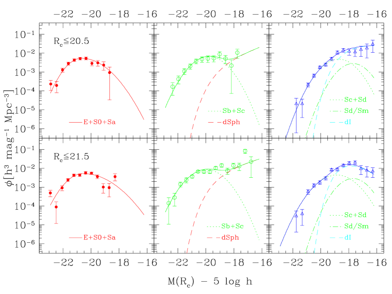
Figure 11: Comparison of the ESO-Sculptor spectral-type luminosity functions for $R_{\mathrm{c}}\leq 20.5$ (top panels) and $R_{\mathrm{c}}\leq 21.5$ (bottom panels) with the composite LFs modeling the intrinsic LFs (see Sandage et al. 1985 and Jerjen & Tammann 1997). Left, center, and right panels show the LFs for the early-type, intermediate-type, and late-type galaxies respectively. Dotted and dot-dashed lines show the adjusted Spiral LFs, and dashed lines show the adjusted dwarf galaxy LFs; solid lines show the composite LFs resulting from the sum of the individual components, excluding the Sd/Sm component, only shown as indicative (see text for details). The respective LF parameters are listed in Table 7 (those for which the “Type of LF” is written in boldface).

As shown in Fig. 2 (Sect. 2.5), the ESS early-type spectral class contains predominantly galaxies with E, S0 and Sa/Sab morphological types (see also Sect. 2.2); the early-type ESS LF can therefore be compared with the sum of the local LFs for these types. We thus perform the STY fit of a two-wing Gaussian to the ESS early-type LF, defined as a Gaussian with a different r.m.s. dispersion ($\Sigma_{1}$ and $\Sigma_{2}$) at the faint and bright ends:

$$\begin{array}[]{ll}\phi(M)dM&=\phi_{0}e^{-X}dM\\ {\rm with}&\\ X&=(M_{0}-M)^{2}/2\Sigma_{1}^{2}\;{\rm for}\;M\leq M_{0}\\ X&=(M_{0}-M)^{2}/2\Sigma_{2}^{2}\;{\rm for}\;M\geq M_{0},\\ \end{array}$$ (15)

For both the $R_{\mathrm{c}}\leq 20.5$ and $R_{\mathrm{c}}\leq 21.5$ samples, shown in the top panels of Fig. 11, the two-wing Gaussian parameterization provides an even better adjustment than with the pure Schechter function (see Fig. 7 for the $R_{\mathrm{c}}\leq 20.5$ sample), as indicated by the larger likelihood ratios (see Table 7). One can also obtain good adjustments of the ESS early-type LF using the sum of the 2 Gaussian functions for the S0 and Sa, and a two-wing Gaussian for the E, with similar peaks but narrower dispersions than for the local LFs in Table 6. Such a multi-component parameterization is however highly degenerate as the relative fractions of E, S0 and Sa in the ESS are poorly determined from the spectral classification, and because the 3 Gaussian components have similar peaks and dispersions: knowledge of the early-type ESS LF is obviously insufficient for constraining separately the E, S0 and Sa LFs. We however adopt the success of a single two-wing Gaussian adjustment, as an indication that the ESS early-type LF is compatible with a mix of E, S0, and Sa galaxies having Gaussian LFs.

Note that the local Gaussian LFs for E, S0 and Sa galaxies (shown in Table 6) have too large a dispersion to match directly the ESS early-type LFs, as the two-wing Gaussian (see Table 7) cannot be fitted by any combination of the mentioned local LFs for either the $R_{\mathrm{c}}\leq 20.5$ or the $R_{\mathrm{c}}\leq 21.5$ sample. Although this could partly originate from evolution and environmental effects, there is a non negligeable contribution from sampling effects. At the faint end, the ESS is limited by its combination of sky coverage and apparent magnitude limit, which results in a small sampling volume: the local LFs for E, S0 and Spiral types in Table 6 are defined out to $M(B_{\mathrm{T}})\sim-15.5$, that is $M(R_{\mathrm{c}})\sim-17.0$, whereas the ESS early-type LF is poorly sampled at $M(R_{\mathrm{c}})$ fainter than $-19.0$ (see histogram in Fig. 7). At the bright end, the steep exponential decrease of the LF causes an under-sampling, because of the limited sky coverage of the survey. Extending the $R_{\mathrm{c}}\leq 20.5$ sample to $R_{\mathrm{c}}\leq 21.5$ (which adds 59 early-type, 66 intermediate-type, and 28 late-type galaxies) is not sufficient to counter-balance this under-sampling, as the deeper sample is only $\sim 52$% complete in redshift measurements (see Table 1). The result of these combined effects is to skew the ESS early-type LF towards bright magnitudes. This effect is observed in most magnitude-limited redshift surveys, and contrasts with the local E LF which is skewed towards faint magnitudes (see Table 6). Jerjen & Tammann (1997) also interpret as incompleteness the early-type LF measured by Muriel et al. (1995), based on the APM survey, which shows a similar behavior: the low luminosity E are compact and could easily be misidentified with stars, even on a 2.5-m high resolution Las Campanas du Pont plate (see Jerjen & Dressler, 1997). Such a bias could also contribute to a narrow dispersion of the early-type LF in the ESS. However, there has been so far no detection of a significant compact population of galaxies which could have been missed in deep redshift surveys (see for example Lilly et al., 1995).

4.4 The ESS intermediate-type luminosity function

For the ESS intermediate-type and late-type LFs, the situation is somewhat different. The ESS intermediate-type class contains predominantly Sb and Sc galaxies (see Sect. 2.5 and Fig. 2b). Sandage et al. (1985) sketch the Sa/Sb and Sc LFs as 2 Gaussian functions with a nearly 1 magnitude brighter peak for the Sc, and a similar r.m.s. dispersion of $\sim 1$ magnitude. Figure 2 suggests that in the ESS intermediate-type class, the Sc are as numerous than the Sb galaxies. Adding to the local Sa/Sb Gaussian LF (as listed in Table 6) a contribution from the Sc local LF would distort the faint end of the Sa/Sb Gaussian. This would however be insufficient to make the flat faint-end observed in the ESS intermediate-type LF for both $R_{\mathrm{c}}\leq 20.5$ and $R_{\mathrm{c}}\leq 21.5$ (see Fig. 11). Moreover, examination of Fig. 3 of Jerjen & Tammann (1997, based on ) shows that both the Sb and Sc LFs decrease to zero galaxies at $M(B_{\mathrm{T}})\simeq-16$, which corresponds to $M(R_{\mathrm{c}})\simeq-17.3$ (using the colors of an Sbc galaxy listed in Table 5), whereas the ESS LF remains flat out to this limit (see Fig. 11).

Having in mind that there are no dwarf Spiral galaxies in the local Universe (see Sandage et al., 1985), and that dwarf spheroidal galaxies have bluer colors than giant E galaxies, we propose that the flat faint-end of the ESS intermediate-type LF is caused by inclusion of dSph galaxies in this class. Indeed, Caldwell (1983) suggests that dE in the Virgo cluster are young and undergo some amount of star formation indicated by an excess of UV light (the so-called “UV upturn phenomenon”): dE with absolute magnitudes $-18\leq M(B_{\mathrm{T}})\leq-16$, that is $-19.7\leq M(R_{\mathrm{c}})\leq 17.7$ for the colors of an E galaxy and $-19.3\leq M(R_{\mathrm{c}})\leq 17.3$ for the colors of an Sbc galaxy (see Table 5), have rest-frame color $0.6\leq U-V\leq 1.3$ (see also the similar results of Caldwell & Bothun 1987 for the Fornax cluster). We thus examine the colors of the $34$ intermediate-type galaxies in the ESS with $-19.5\leq M(R_{\mathrm{c}})\leq-17.5$. Figure 9 indicates these galaxies have redshifts in the interval $0.07\leq z\leq 0.25$, with a median redshift $\sim 0.18$. Their apparent colors describe the interval $0.6\leq B-R_{\mathrm{c}}\leq 2.0$, with 73% of the galaxies in the interval $0.9\leq B-R_{\mathrm{c}}\leq 1.5$. There is therefore ample overlap for a population of dE galaxies with rest-frame color $0.6\leq U-V\leq 1.3$, as $U-V$ shifts approximately into $B-R_{\mathrm{c}}$ at $z\sim 0.2$. Independent evidence is brought by the actual spectra of dE in the Fornax cluster, obtained by Held & Mould (1994): these spectra show only a weak or a non-existing break at the location of the H & K CaII lines (3933 and 3968 Å), and display intermediate-color continua which makes them closely resemblant to Sa and Sb spectra (Kennicutt, 1992). If such dwarf Spheroidal galaxies were present in the ESS, they would be classified as intermediate-type galaxies by the PCA spectral classification (see Sect. 2.2 and Galaz & de Lapparent 1998).

We therefore choose to parameterize the ESS intermediate-type LF by the sum of a Gaussian LF, modeling the contribution from Sb+Sc galaxies, and a Schechter component modeling the contribution from dwarf galaxies. Similarly to the two-wing Gaussian in Eq. 15, the Gaussian LF is defined as

$$\phi(M)dM=\phi_{0}e^{-(M_{0}-M)^{2}/2\Sigma^{2}}dM;$$ (16)

the Schechter LF is defined in Eq. 14. The Gaussian+Schechter composite LF function has 5 free parameters: the peak $M_{0}$ and r.m.s. dispersion $\Sigma$ of the Gaussian, the parameters $M^{*}$ and $\alpha$ of the Schechter function, and the ratio $\phi_{0}/\phi^{*}$ of the amplitudes for the 2 functions.

A general STY fit with all parameters left free is highly unstable and yields various unrealistic solutions. We however find that fixing the value $\phi_{0}/\phi^{*}$ is a sufficient constraint for the fit to converge towards a stable and realistic solution. We therefore perform iterative fits in which the ratio $\phi_{0}/\phi^{*}$ is fixed to a series of values separated by some increment; the smallest increments, used near the maximum of likelihood ratio, are $0.01$. The best fit is then defined as the STY solution with the largest likelihood ratio. In the following, we denote these fits the “iterative” STY solutions, or “iterative fits”.

The parameters resulting from the iterative fits for the $R_{\mathrm{c}}\leq 20.5$ and $R_{\mathrm{c}}\leq 21.5$ samples are listed in Table 7, just below the corresponding “Pure Schechter” fits. The iterative composite fits of the ESS intermediate-type LF provide as good adjustments as the pure Schechter fits: the likelihood ratios only show a small decrease, from $0.75$ to $0.72$ for the $R_{\mathrm{c}}\leq 20.5$ sample, and from $0.83$ to $0.78$ for the $R_{\mathrm{c}}\leq 21.5$ sample. We have not directly estimated the uncertainty in the likelihood ratios, but results for fits with similar LF parameters for the Gaussian and Schechter components (within 1%) yield changes in the likelihood ratio by as much a $0.03$, which provides an underestimate of the true error. The decrease in the likelihood ratios from the pure Schechter fits to the iterative fits are therefore within the $\sim 1$-$\sigma$ error bars.

In the iterative fit of the intermediate-type LF from the $R_{\mathrm{c}}\leq 21.5$ sample, the value $M^{*}(R_{\mathrm{c}})=-20.58$ is abnormally bright for field dSph galaxies, expected to represent a significant population in the ESS: as shown by Binggeli et al. (1990, see their Fig. 10, bottom panel), field dSph galaxies might be fainter than in the Virgo and Centaurus clusters, with $M(B_{\mathrm{T}})\ga-17$. We therefore re-run the STY solution for the $R_{\mathrm{c}}\leq 21.5$ sample, with the added constraint that $M^{*}(R_{\mathrm{c}})\ga-19.43$ (the measured value from Virgo, which is also fainter than for Centaurus, see Table 6). When using this constraint on $M^{*}$, their is no need to perform iterative fits with varying values of $\phi_{0}/\phi^{*}$: leaving all parameters free yields a stable minimum with $M^{*}(R_{\mathrm{c}})=-18.98\pm 0.37$ and $\alpha=-1.53\pm 0.33$ (other parameters are listed in Table 7). The likelihood ratio decreases to $0.62$, a lower but still acceptable value. Because the $M^{*}(R_{\mathrm{c}})\ga-19.43$ constrained fit to the $R_{\mathrm{c}}\leq 21.5$ sample provides shape parameters for the Gaussian and Schechter components ($M_{0}$, $\Sigma$, $M^{*}$ and $\alpha$) which agree at less than the 1-$\sigma$ level with those for the iterative fit to the $R_{\mathrm{c}}\leq 20.5$ sample (the uncertainties in 2 measures are added in quadrature in order to estimate the uncertainty in the difference), we adopt these 2 fits and plot them in the lower and upper middle panels of Fig. 11 resp. (green dotted lines for the Sb+Sc LF, red dashed line for the dSph LF); the sum of the Gaussian and Schechter components are plotted as continuous green lines. The amplitude of each iterative fit is determined by least-square adjustment to the corresponding SWML solution (see Sect. 4.1).

The values of $M_{0}$ for the Gaussian component which models the Sb+Sc contribution to the intermediate-type LF in the $R_{\mathrm{c}}\leq 20.5$ and $R_{\mathrm{c}}\leq 21.5$ samples, $M_{0}(R_{\mathrm{c}})=-19.79\pm 0.29$ and $M_{0}(R_{\mathrm{c}})=-19.97\pm 0.21$ resp., are both close to that listed in Table 6 for the Sc galaxies in the $R_{\mathrm{c}}$ filter, $M_{0}(R_{\mathrm{c}})=-19.8$. Moreover, Fig. 3 of Jerjen & Tammann (1997) shows that the Sb LF may have a similar magnitude distribution as the Sc LF, in both the Centaurus and Virgo clusters, whereas the Sa LF has a brighter peak in both clusters. The local intrinsic LF for Sc galaxies can therefore be used to model the Sb+Sc LF, thus validating our interpretation of the Gaussian component of the ESS intermediate-type LF as due to Sb+Sc galaxies. This in turn suggests that the Spiral galaxies detected in the Centaurus and Virgo cluster may be representative of those detected in the ESS.

The r.m.s. dispersion $\Sigma$ of the Sb+Sc Gaussian component is $0.88\pm 0.17$ for the $R_{\mathrm{c}}\leq 20.5$ sample, and $0.91\pm 0.18$ for $R_{\mathrm{c}}\leq 21.5$. These 2 values are in good agreement, with a $0.12$-$\sigma$ difference. They are however smaller than the dispersion $\Sigma\sim 1.2$ for the local Sc LF (see Table 6). As shown in Fig. 2b, only the Sc galaxies of earliest spectral type are included in the intermediate-type class. A narrower dispersion might be expected for this sub-population. It is also likely that a significant part of the difference with the ESS dispersion $\Sigma\sim 0.9$ results from the selection effects discussed in Sect. 4.3, which cause under-sampling at both the bright and faint ends of the ESS LFs.

The central panels of Fig. 11 show that both the characteristic magnitude $M^{*}$ and the faint-end slope $\alpha$ of the dSph Schechter component are poorly constrained by the intermediate-type LFs, in contrast to the Gaussian component. The effect on $\alpha$ is more acute for the $R_{\mathrm{c}}\leq 20.5$ sample, as the SWML solution has only few points fainter than the peak of the Gaussian component. For the $R_{\mathrm{c}}\leq 21.5$, the SWML solution reaches nearly one magnitude fainter, to $M(R_{\mathrm{c}})\sim-16.5$, thus putting tighter constraints on $\alpha$. The differing value of $M^{*}$ by $\sim 1.6^{\mathrm{mag}}$ obtained for the $R_{\mathrm{c}}\leq 21.5$ sample using the iterative fit and the $M^{*}\ga-19.43$ constrained fit resp. (see Table 7) illustrate the difficulty in constraining $M^{*}$.

Conversion into the $B_{\mathrm{T}}$ band of $M^{*}(R_{\mathrm{c}})\simeq-19$, obtained from the iterative fit to the $R_{\mathrm{c}}\leq 20.5$ sample, and from the $M^{*}\ga-19.43$ constrained fit to the $R_{\mathrm{c}}\leq 21.5$ sample, yields $M^{*}(B_{\mathrm{T}})\simeq-17.3$ (as in Table 6, we use the color term for Sab galaxies listed in Table 5). We recall that in the ESS, the LF for the dSph is expected to result from the combination of the LFs for dSph in groups and in the field (see Sect. 4.2); $M^{*}(B_{\mathrm{T}})\simeq-17.3$ is indeed intermediate between the values for the Virgo and Centaurus clusters listed in Table 6, and the fainter value suggested by field dSph galaxies in the Ursa Major cloud (see Fig. 10 of Binggeli et al., 1990). We therefore adopt as a likely characterization of the dSph component included in the ESS intermediate-type LF that derived from the $R_{\mathrm{c}}\leq 21.5$ sample, with $M^{*}(R_{\mathrm{c}})=-18.98\pm 0.37$ and $\alpha=-1.53\pm 0.33$. Note however that, even in the $R_{\mathrm{c}}\leq 21.5$ sample, the large uncertainty $\sigma(\alpha)=0.33$ makes the faint-end slope of the dSph LF component derived from the ESS compatible with those derived from both the Centaurus and Virgo clusters, at less than the 1-$\sigma$ level.

4.5 The ESS late-type luminosity function

We propose a similar parameterization for the ESS late-type LF as for the intermediate-type LF. Figure 2 suggests that the ESS late-type class contains predominantly Sc and Sd/Sm galaxies. Although the Sc and Sd/Sm populations can be modeled as 2 separate Gaussian LFs with the Sd/Sm LF shifted to fainter magnitudes (see Table 6 and Sandage et al., 1985), Fig. 3 of Jerjen & Tammann (1997) shows that the magnitude distribution of the Sd/Sm galaxies, is included in that for the Sc galaxies. The contribution from Sd/Sm galaxies can therefore conveniently be included into the Sc LF, and we denote Sc+Sd this joint LF. We then model the ESS late-type LF as the composite sum of a Gaussian LF for the Sc+Sd galaxies, and a Schechter function for the Im+BCD galaxies (denoted dI). We then show a posteriori that the contribution from Sd/Sm galaxies to the composite function modeling the ESS late-type LF is negligeable, as it is dominated at all magnitudes considered by the contribution from either the Sc or the dI galaxies.

The right panels of Fig. 11 show the iterative STY fits of the Gaussian+Schechter composite LF to the late-type galaxies with $R_{\mathrm{c}}\leq 20.5$ and $R_{\mathrm{c}}\leq 21.5$; the Sc+Sd LFs are shown as dotted lines, and the dI LFs as dashed lines (the corresponding parameters are listed in Table 7). The increased values of the likelihood ratios ($0.59$ and $0.61$ resp.) compared with the values for the pure Schechter fits ($0.46$ and $0.51$ resp.) show that the composite fits are better descriptions of the ESS late-type LFs. Moreover, the fitted Gaussian peak for the Sc+Sd component in both the $R_{\mathrm{c}}\leq 20.5$ and $R_{\mathrm{c}}\leq 21.5$ samples ($-18.72\pm 0.34$ and $-18.86\pm 0.29$) is remarkably close to the mean value of $M_{0}(R_{\mathrm{c}})$ for the Sc and Sd/Sm local LFs, $M_{0}(R_{\mathrm{c}})=-18.75$ (see Table 6).

The measured dispersion of the Sc+Sd Gaussian component is $\Sigma=0.86\pm 0.14$ and $\Sigma=0.97\pm 0.13$ for the $R_{\mathrm{c}}\leq 20.5$ and $R_{\mathrm{c}}\leq 21.5$ LFs resp., which agree at less than $\sim 1$-$\sigma$. Values of $1.2\pm 0.1$ and $0.8\pm 0.1$ are however listed in Table 6 for the Sc, and Sd/Sm components respectively. As for the intermediate-type LF (Sect. 4.4), only part of the Sc galaxies are expected to be included in the late-type class, those of later spectral-type (see Fig. 2a), and this sub-class may have a narrower dispersion than the full Sc population. The already mentioned sampling effects which bias the Gaussian dispersion towards low values might also affect the ESS late-type LF (see Sect. 4.3).

The STY composite fits of the late-type LF yield values of $M^{*}(R_{\mathrm{c}})$ for the dI Schechter component which are in agreement for the $R_{\mathrm{c}}\leq 20.5$ and $R_{\mathrm{c}}\leq 21.5$ samples ($M^{*}[R_{\mathrm{c}}]$ differs by less than $\sim 1$-$\sigma$), with a mean value $M^{*}(R_{\mathrm{c}})\simeq-17.7$. This value is intermediate between the values for the Virgo and Centaurus cluster (see Table 6). Moreover, the faint value $M^{*}(R_{\mathrm{c}})=-16.74$ measured from the Virgo cluster (Jerjen & Tammann, 1997) can be excluded: whatever the dispersion of the Gaussian LF for the Sc+Sd galaxies, and whatever the slope $\alpha$ for the dI component, a faint $M^{*}(R_{\mathrm{c}})$ prevents from adjusting simultaneously the ESS late-type LF in the intervals $-19\leq M(R_{\mathrm{c}})\leq-18$ and $-18\leq M(R_{\mathrm{c}})\leq-16$. Conversion of $M^{*}(R_{\mathrm{c}})\simeq-17.7$ into the $B_{\mathrm{T}}$ band yields $M^{*}(B_{\mathrm{T}})\simeq-17.1$ (as in Table 6, we use the color term for Sm/Im galaxies listed in Table 5). This value appears consistent with that suggested by field dI galaxies in the Ursa Major cloud (see Fig. 10 of Binggeli et al., 1990).

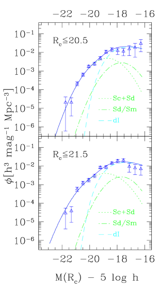
Figure 12: Other composite fits of the ESO-Sculptor late-type luminosity functions for the $R_{\mathrm{c}}\leq 20.5$ and $R_{\mathrm{c}}\leq 21.5$ samples. Dotted and dot-dashed lines show the Spiral LFs, dashed lines show the dwarf galaxy LFs (dI). Solid lines show the composite LFs resulting from the sum of the individual components, except for the Sd/Sm component only shown as indicative (see text for details). Here, the Schechter slope $\alpha$ of the dI component is fixed to $-0.3$, as measured from the Virgo cluster (see Tables 6 and 7). The other LF parameters are listed in Table 7.

In contrast, the values of $\alpha$ for the dI Schechter component of the ESS late-type LF differ by $3.6$-$\sigma$ for the $R_{\mathrm{c}}\leq 20.5$ and $R_{\mathrm{c}}\leq 21.5$ samples: the slopes are $\alpha=-0.83\pm 0.26$ and $\alpha=0.39\pm 0.21$ respectively. The Centaurus slope $\alpha=-1.35$ (see Table 6) is too steep to match the LF of either sample, whereas the slope $\alpha=-0.31$ measured from the Virgo cluster is acceptable for both samples: by fixing $M_{0}(R_{\mathrm{c}})$ and $\Sigma$ for the Gaussian component to the best fit values obtained in the iterative fits (Table 7), and the Schechter slope $\alpha$ to $-0.30$, the STY solution yields values of $M^{*}(R_{\mathrm{c}})$ which differ by less than 1-$\sigma$ for the $R_{\mathrm{c}}\leq 20.5$ and $R_{\mathrm{c}}\leq 21.5$ samples (and by $\sim 1$-$\sigma$ from the respective values obtained by the iterative STY fits); the corresponding likelihood ratios are $0.41$ and $0.44$ (the parameters for these constrained fits are listed in Table 7 just after the iterative fits, and are plotted in Fig. 12). Similar likelihood ratios are also obtained when $\alpha$ is fixed to $-0.40$: $0.43$ and $0.42$ for the $R_{\mathrm{c}}\leq 20.5$ and $R_{\mathrm{c}}\leq 21.5$ samples respectively. For $\alpha\leq-0.50$ or $\alpha\geq-0.20$, the likelihood ratios for the 2 samples differ by at least $0.6$. Also, although the redshift incompleteness is corrected for in the calculation of the SWML solution (see Sect. 3.1), the low amplitude of the faintest 3 points in the $R_{\mathrm{c}}\leq 21.5$ LF, which causes the high value $\alpha=0.39\pm 0.21$, could be explained by a differential bias against late morphological type at this faint limit: beyond the nominal limit of $R_{\mathrm{c}}\leq 20.5$, objects with preferentially steeper light profile were observed, in order to insure a sufficient signal-to-noise ratio in the spectra; these objects are likely to have an earlier morphological type.

Using the faint-end slope $\alpha=-0.83$ obtained for the $R_{\mathrm{c}}\leq 20.5$ sample as the steeper allowed value, and the common value $\alpha=-0.3$ as an upper limit, we obtain the constraint that the faint-end slope of the ESS late-type dwarf component lies in the interval $-0.8\la\alpha\la-0.3$. However, as for the intermediate-type LF, the ESS weakly constrains the faint-end slope of the dI component, and we regard these limits on $\alpha$ as tentative.

To evaluate contribution from the Sd/Sm galaxies to the ESS late-type LF, we also plot in the right panels of Figs. 11 and in Fig. 12 the expected Sd/Sm LF with the shape listed in Table 6 and the amplitude $\phi_{0}$ defined such as the integral over the Sd LF is half the integral over the Sc+Sd LF for $M(R_{\mathrm{c}})\leq-16.6$. We justify this choice a follows:

• Fig. 3 of Jerjen & Tammann (1997) shows that for $M(B_{\mathrm{T}})\leq-15.5$, the Sd/Sm galaxies amount to approximately half the number of Sc galaxies;

• $M(B_{\mathrm{T}})\leq-15.5$ corresponds to $M(R_{\mathrm{c}})\leq-16.6$ when using $M(B_{\mathrm{T}})-M(R_{\mathrm{c}})=1.1$ for an Scd galaxy (see Table 5);

• if one assume that about half of the Sc galaxies are included in each of the ESS intermediate and late-type classes, the Sc galaxies then contribute in equal amount as the Sd/Sm galaxies to the late-type LF, and the expected ratio of Sd over Sc+Sd galaxies with $M(R_{\mathrm{c}})\leq-16.6$ is approximately $0.5$.

The resulting amplitudes $\phi_{0}$ for the Sd/Sm LF in the $R_{\mathrm{c}}\leq 20.5$ and $R_{\mathrm{c}}\leq 21.5$ are listed in Table 7. Figures 11 or 12 show that in the full magnitude range considered, the Sd/Sm component is a factor $\sim 10$ smaller than the late-type LF. This confirms a posteriori that the Sd/Sm galaxies have a negligeable contribution to the ESS late-type LF, and could not be constrained as a separate component in the composite fits.

4.6 The ESS peak surface brightness distributions

We now use the surface brightness (SB) of the ESS galaxies to provide further evidence for the contribution of dwarf galaxies to both the intermediate-type and late-type classes. The SExtractor package (Bertin & Arnouts, 1996) was used for image analysis of the ESS photometric survey (Arnouts et al., 1997), and among the extracted parameters is the peak SB of the objects, calculated in the one object pixel with the highest flux. Galaz et al. (2002) show that the central SB in the near-infrared is strongly correlated with fundamental physical parameters for low-SB galaxies. Extrapolating this result to optical wavelengths, we use for each galaxy in the ESS its SExtractor peak SB in the $R_{\mathrm{c}}$ band (denoted $SB_{\mathrm{peak}}$) and correct it for (i) the K-correction of the corresponding galaxy, and (ii) the dimming due to the expansion of the Universe, which varies with redshift $z$ as $2.5\log(1+z)^{4}$; across the ESS survey, the SB dimming varies from $0.41^{\mathrm{mag}}$ at $z=0.1$ to $2.04^{\mathrm{mag}}$ at $z=0.6$. We obtain a “rest-frame” peak SB defined as

$$SB_{\mathrm{peak/rest}}=SB_{\mathrm{peak}}-10\log(1+z)-K(z,\delta^{\prime})$$ (17)

(see Sect. 2.3 for the definition of the K-correction $K[z,\delta^{\prime}]$). The resulting $SB_{\mathrm{peak/rest}}$ describes the interval $18\la\mu_{0}\la 22.5$ mag arcsec^-2 in the $R_{\mathrm{c}}$ band for the 617 ESS galaxies with $R_{\mathrm{c}}\leq 20.5$.

These values of the rest-frame peak SB cannot however be directly compared among them, because the peak pixel over which they are calculated corresponds to a varying physical aperture at different redshifts. Moreover, as 2 different telescopes and 4 different CCDs were used over the course of the photometric survey (Arnouts et al., 1997), with pixels scales of 0.35 arcsec/pixel, 0.44 arcsec/pixel, and 0.675 arcsec/pixel in the $R_{\mathrm{c}}$ filter, the physical transverse size over which the rest-frame peak SB is calculated can take 3 different values at a given redshift. We thus calculate for each objet the physical transverse “radius” of the peak pixel, denoted $r_{\mathrm{peak}}$, and defined as the product of half the pixel size $A_{\mathrm{pix}}$ (in radians) by the angular-distance diameter $d_{\mathrm{D}}=d_{\mathrm{L}}/(1+z)^{2}$, where $d_{\mathrm{L}}$ is the luminosity distance given in Eq. 7. The resulting values of $r_{\mathrm{peak}}$ vary from $\sim 0.15$$h^{-1}$ kpc at $z\simeq 0.05$ to $\sim 0.5$$h^{-1}$ kpc, $\sim 0.6$$h^{-1}$ kpc, $\sim 0.95$$h^{-1}$ kpc at $z\simeq 0.3$, and to $\sim 0.65$$h^{-1}$ kpc, $\sim 0.85$$h^{-1}$ kpc, $\sim 1.3$$h^{-1}$ kpc at $z\simeq 0.6$ (the 3 values correspond to the 3 above mentioned pixel sizes).

These variations in $r_{\mathrm{peak}}$ for the ESS result in significant variations in the average SB measured within the peak pixel: for example, as shown by Binggeli & Cameron (1991), the SB profile of giant and dwarf Elliptical galaxies in the Virgo cluster steeply decreases outwards, and varies by $\sim 3$ to $\sim 5$ magnitudes when the physical radius varies from $\sim 0.5$$h^{-1}$ kpc to $\sim 1.5$$h^{-1}$ kpc (see also Binggeli & Jerjen, 1998). For comparison of the rest-frame peak SB among the 3 spectral classes, we therefore separate galaxies within each spectral class into the following 3 intervals of $r_{\mathrm{peak}}$: $r_{\mathrm{peak}}\leq 0.6$$h^{-1}$ kpc, $0.6<r_{\mathrm{peak}}\leq 0.8$$h^{-1}$ kpc, and $r_{\mathrm{peak}}>0.8$$h^{-1}$ kpc; these values are chosen so that there are more than $40$ galaxies in each sub-sample of each spectral class. Note that the variable seeing conditions during the course of the survey also affect the measured peak SB. Seeing is most effective in decreasing the peak SB of objects with steep profiles, thus decreasing the contrast between objects with high and low peak SB. The segregation between galaxies with high and low peak SB detected in Fig. 13 below might thus be intrinsically larger.

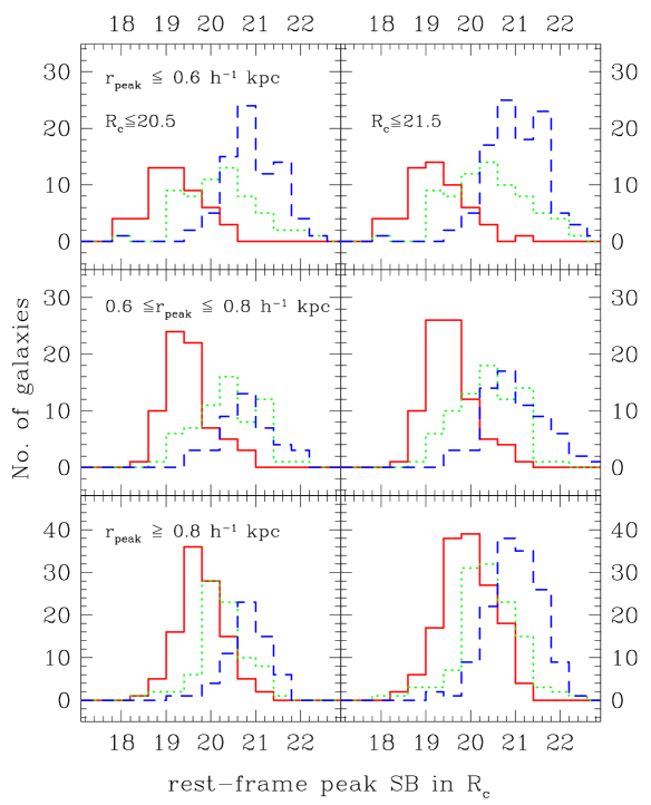
Figure 13: Comparison of the ESO-Sculptor rest-frame peak surface brightness at $R_{\mathrm{c}}\leq 20.5$ (3 left panels) and $R_{\mathrm{c}}\leq 21.5$ (3 right panels), for the early-type (red solid line), intermediate-type (green dotted line), and late-type (blue dashed line) galaxies, using redshift increments $\Delta z=0.04$. The 3 spectral classes are separated according to the physical radius $r_{\mathrm{peak}}$ of the peak pixel over which is calculated the surface brightness: top, middle, and bottom panels correspond to $r_{\mathrm{peak}}\leq 0.6$$h^{-1}$ kpc, $0.6<r_{\mathrm{peak}}\leq 0.8$$h^{-1}$ kpc, and $r_{\mathrm{peak}}>0.8$$h^{-1}$ kpc respectively.

Figure 13 shows the resulting histograms of rest-frame peak SB for the 3 intervals of $r_{\mathrm{peak}}$ within each ESS spectral class, for $R_{\mathrm{c}}\leq 20.5$ and $R_{\mathrm{c}}\leq 21.5$. For $r_{\mathrm{peak}}\leq 0.6$$h^{-1}$ kpc and $0.6<r_{\mathrm{peak}}\leq 0.8$$h^{-1}$ kpc (top and middle panels), the intermediate-type and late-type galaxies with $R_{\mathrm{c}}\leq 20.5$ show a low SB tail, which is not present in the early-type galaxies. For $r_{\mathrm{peak}}>0.8$$h^{-1}$ kpc , the effect is only visible for the late-type galaxies. For all 3 intervals of $r_{\mathrm{peak}}$, the effect persists at $R_{\mathrm{c}}\leq 21.5$, with a larger fraction of galaxies in the low-SB tails. The absence of low-SB tail for the intermediate-type galaxies with $r_{\mathrm{peak}}>0.8$$h^{-1}$ kpc can be explained as follows: the ESS galaxies with $r_{\mathrm{peak}}>0.8$$h^{-1}$ kpc have $z\ga 0.25$, and are therefore brighter than $M(R_{\mathrm{c}})\simeq-19.2$, due to their K-corrections (see Fig. 9 in Sect. 3.2 above). However, as shown in Fig. 11, the early-type dwarf contribution to the intermediate-type LF becomes dominant only at fainter magnitudes than this limit. The early-type dwarf galaxies are therefore inherently excluded from the $r_{\mathrm{peak}}>0.8$$h^{-1}$ kpc sub-samples, which in turn explains the absence of the low SB tails for these samples. This selection effect has a smaller impact on the late-type galaxies, as these have a smaller K-correction, and a steeply increasing LF at $M(R_{\mathrm{c}})\simeq-19.0$: a non-negligeable fraction of the late-type galaxies are thus included in the $r_{\mathrm{peak}}>0.8$$h^{-1}$ kpc samples, at both $R_{\mathrm{c}}\leq 20.5$ and $R_{\mathrm{c}}\leq 21.5$.

We also observe a correlation between SB and $M(R_{\mathrm{c}})$ magnitude for the ESS galaxies in both the $r_{\mathrm{peak}}\leq 0.6$$h^{-1}$ kpc and $0.6<r_{\mathrm{peak}}\leq 0.8$$h^{-1}$ kpc sub-samples, with fainter galaxies having fainter SB. The galaxies with low SB detected in both the intermediate-type and late-type galaxies are therefore low luminosity objects. This provides further evidence that the faint components of the ESS intermediate-type and late-type LFs are indeed dwarf galaxies, characterized by both low luminosity and low SB.

For the reasons discussed above, the measured peak SB for the ESS galaxies cannot be directly compared with the SB measurements derived from nearby galaxies. For example, in the Sculptor and Centaurus A groups, Jerjen et al. (2000) derive the extrapolated central SB calculated by adjustment of Sérsic models to the object profiles: this yields relatively bright SB. For the Virgo cluster, Binggeli & Cameron (1991) calculate the mean SB within the effective radius defined to contain half of the total light of the galaxy, which varies by a factor of 3 among the populations of Virgo giant/dwarf Elliptical and Lenticular galaxies (see their Fig. 1). The ESS results can however be compared with the results of Trentham & Hodgkin (2002), who measure the average $B$ band SB of Virgo cluster galaxies within a constant circular aperture of 6 arc-second radius: at the redshift of Virgo ($z\simeq 0.0038$), this corresponds to $0.33$$h^{-1}$ kpc. The values of SB measured by Trentham & Hodgkin (2002) can thus be compared with those for the ESS galaxies in the $r_{\mathrm{peak}}\leq 0.6$$h^{-1}$ kpc sub-sample. As in the ESS, Trentham & Hodgkin (2002) show a tight correlation between SB and absolute magnitude, with brighter galaxies having brighter SB (see also Binggeli & Cameron 1991; Jerjen et al. 2000): the E/S0 and Spiral galaxies populate the bright part of the Virgo sequence in the SB interval $\sim 18-23B$ mag arcsec^-2 for Virgo, and the early-type and late-type dwarf galaxies populate the faint part of the sequence, with $\sim 21-27B$ mag arcsec^-2. At a SB of $\geq 22B$ mag arcsec^-2, the dwarf galaxies dominate in numbers over the giant galaxies. This limit corresponds to $\sim 20.7R_{\mathrm{c}}$ mag arcsec^-2 for a dE galaxy, assuming the color of an Sab galaxy (see Table 6), and to $\sim 21.4R_{\mathrm{c}}$ mag arcsec^-2 for an Im galaxy (see Table 5). Interestingly, the SB histograms for the ESS intermediate-type and late-type galaxies with $r_{\mathrm{peak}}\leq 0.6$$h^{-1}$ kpc in Fig. 13 both show a local peak (at faint SB) within less than $0.2^{\mathrm{mag}}$ from these values; the sharp decrease in objects fainter than these peaks is caused by incompleteness. This comparison thus provides evidence that the low SB tails of the ESS intermediate-type and late-type classes contain dwarf galaxies similar to those detected in nearby clusters as Virgo.

In Fig. 13, the variations in the SB distributions as a function of $r_{\mathrm{peak}}$ also provide evidence of varying profiles among the ESS galaxies. When going to larger values of $r_{\mathrm{peak}}$, the SB histograms for the intermediate-type and late-type galaxies maintain a nearly constant median value of SB, whereas the early-type galaxies show a shift to fainter SB. This can be interpreted as a signature of the steeper profiles for E galaxies, which according to Binggeli & Jerjen (1998) have Sérsic parameter $n=0.1$ to $0.5$; in contrast, Binggeli & Jerjen (1998) show that the SB profile of the early-type/late-type dwarf and the Spiral galaxies are better fitted by flatter profiles, with $0.3\la n\la 2.0$ ($n=0.25$ corresponds to the $r^{1/4}$ law by de Vaucouleurs 1948; $n=1$ corresponds to an exponential profile, as measured by Freeman 1970, for the disk component of Spiral and S0 galaxies). The effect can be interpreted as follows: for smaller values of $r_{\mathrm{peak}}$, steeper parts of the SB profile of E galaxies are sampled, and brighter values of SB are derived. The S0 and Sa galaxies also included in the early-type class might also contribute to the effect, as the bulges have a significant contribution to the object profile in the central parts of the galaxies.

5 Conclusions and prospects

The present analysis of the ESO-Sculptor Survey (ESS) provides new measurements of the $B$, $V$, and $R_{\mathrm{c}}$ luminosity functions (LF) of galaxies at $z\la 0.6$. We use a PCA-based spectral classification, and a technique providing a parametric estimation of the K-corrections as a function of redshift and spectral type. From these, we derive absolute magnitudes accurate to $0.09^{\mathrm{mag}}$ in $R_{\mathrm{c}}$, $0.13^{\mathrm{mag}}$ in $V$, and $0.16^{\mathrm{mag}}$ in $B$ for the nearly complete sample of 617 galaxies with redshift at $R_{\mathrm{c}}\leq 20.5$. The LFs are then calculated for 3 spectral-type sub-samples with comparable numbers of galaxies, denoted early-type, intermediate-type, and late-type respectively. Projection of the Kennicutt (1992) galaxies onto the ESS spectral sequence shows that the 3 spectral classes correspond to morphological types E/S0/Sa, Sb/Sc, and Sc/Sm/Im respectively.

The derived LFs for each spectral type have a similar behavior in the $B$, $V$ and $R_{\mathrm{c}}$ bands, which indicates that they measure physical properties of the underlying galaxy populations. They are well fitted by Schechter functions, with a dimming of the bright-end and a steepening of the faint-end when going from early-type to late-type galaxies. Because the spectroscopic sample was selected in the $R_{\mathrm{c}}$ band, the $V$ and $B$ band LFs suffer from incompleteness in blue galaxies at the faint limit; this bias tends to weaken the steepening of the faint-end of the LF for late-type galaxies.

We then compare the ESS spectral-type LFs with the results from the comparable CNOC2 redshift survey (Lin et al., 1999), the only other redshift survey to similar depth and based on a spectral classification. The Schechter fits to the ESS LFs in the $B$ and $R_{\mathrm{c}}$ bands are in agreement with those from the CNOC2. In the $V$ band, the ESS provides the first estimates of intrinsic LFs at $z\sim 0.3$. Further comparison of the ESS with other redshift surveys is reported in de Lapparent (2003), in which is performed a detailed analysis of all the existing measurements of intrinsic LFs in the $UBVR_{\mathrm{c}}I_{\mathrm{c}}$ bands from redshift surveys with effective depth ranging from $z\simeq 0.03$ to $0.6$. By using the local intrinsic LFs per morphological type as a reference, de Lapparent (2003) shows how the existing redshift surveys may mix galaxies of different morphological types, thus complicating the interpretation of their LFs.

The salient results of the present article are obtained by fitting the 3 ESS spectral-type LFs in the $R_{\mathrm{c}}$ band with composite functions suggested by the intrinsic LFs measured locally for each morphological type in the Virgo, Centaurus, and Fornax clusters (Sandage et al., 1985; Jerjen & Tammann, 1997). Specifically, we show that the ESS spectral-type LFs can be modeled as follows:

• the early-type LF: by a two-wing Gaussian function representing the contributions from E, S0, and Sa galaxies;

• the intermediate-type LF: by the sum of a Gaussian function representing the Sb+Sc galaxies, and a Schechter function with a steep slope ($\alpha\la-1.5$) representing the contribution from dwarf Spheroidal galaxies, which dominates at $M(R_{\mathrm{c}})\ga-19.0$.

• the late-type LF: by the sum of a Gaussian function for the Sc+Sd galaxies, and a Schechter function with a flat or weaker slope ($-0.8\la\alpha\la-0.3$) representing the dwarf Irregular galaxies, which dominate at $M(R_{\mathrm{c}})\ga-19.0$.

The interesting aspect of the comparison of the ESS spectral-type LFs with the local intrinsic LFs is that it provides clues on the various galaxy populations included in the ESS spectral classes. It first shows that the bright end of the 3 spectral-type LFs is dominated by giant galaxies (E, S0, Spirals). It also reveals the contribution from dwarf galaxies to the faint-end of both the ESS intermediate-type and late-type LFs. These dwarf galaxies lie at $z\la 0.2$ and are characterized by low luminosity ($M[R_{\mathrm{c}}]\ga-18.5$) and low surface brightness ($\ga 20.5$ $R_{\mathrm{c}}$ mag arcsec^-2 averaged within a physical radius of $0.6-0.8$$h^{-1}$ kpc). This interpretation of the ESS spectral-type LFs illustrates how a spectral classification may mix galaxies of different morphological type: the ESS intermediate-type class may contain both Spiral (Sb+Sc) galaxies and dwarf Spheroidal galaxies.

Comparison of the ESS LF components for the various morphological types with the local intrinsic LFs by Sandage et al. (1985) and Jerjen & Tammann (1997) suggests that the shape of the LFs for the individual Hubble types might not vary markedly in the redshift interval $0\la z\la 0.6$: contributions from Gaussian LFs for giant galaxies (E, S0, Sa, Sb, Sc) with similar peak magnitudes as locally can be adjusted to the ESS LFs. The systematically narrower dispersion for the ESS Gaussian components can be explained by selection effects inherent to magnitude-limited redshift surveys, which cause under-sampling at both the bright-end and faint-end of the ESS LFs. A contribution from environmental effects is also expected, such as the presence of brighter giant galaxies in clusters than in sparse groups and the field, due to the higher frequency of merging and cannibalism in dense regions. The same dimming of the characteristic luminosity which is observed locally when going to later Spiral type (from Sa, to Sb, Sc, and Sd/Sm) is observed in the ESS. Because late-type Spiral galaxies are brightened in the optical by their higher star formation rates compared with early-type Spiral galaxies, their dimming in luminosity is indicative of a systematic decrease in mass.

For the dwarf galaxies, the ESS composite fits suggest a steeper slope for the early-type dwarf LF ($\alpha\ga-1.5$) than for the late-type dwarf LF ($\-0.8\la\alpha\la-0.3$), as already detected in several nearby groups and clusters (Sandage et al., 1985; Jerjen & Tammann, 1997; Jerjen et al., 2000). This confirms earlier suggestions that the late-type dwarf LF is bounded at the faint-end (Sandage et al., 1985; Jerjen et al., 2000). Nevertheless, the ESS only probes the brightest part of the dwarf galaxy LFs, to $M(R_{\mathrm{c}})\leq-16$, and therefore puts poor constraints on their actual slope faint-end slope. The characteristic magnitude $M^{*}$ of the Schechter LFs for the dwarf galaxies is also poorly constrained by the composite fits. We thus emphasize that due to the various incompleteness effects, the specific ESS composite fits should not be used as quantitative constraints on the intrinsic LFs at $z\sim 0.3$. These fits should rather be considered as indicative of the possibilities expected by application to forthcoming larger samples. These limitations point to the need for field measurements based solely on dwarf galaxy samples.

Recent results do provide information on the local dwarf galaxy LFs at faint magnitudes. In their study which combines all available data on dwarf galaxies in the Sculptor, Centaurus A, and M81 groups, together with the Local Group, Jerjen et al. (2000) measure a steep slope $\alpha=-1.29\pm 1.10$ for dwarf galaxies brighter than $M(B_{\mathrm{T}})=-14.0$; in these data, late-type dwarf galaxies dominate over early-type dwarf for $M(B_{\mathrm{T}})\leq-14.0$, and early-type dwarf galaxies represent an increasing proportion at fainter magnitudes (out to $M[B_{\mathrm{T}}]\simeq-9.0$); in these data, the LF for the late-type dwarf galaxies reaches its maximum in a “plateau” located in the interval $-16\leq M(B_{\mathrm{T}})\leq-14$ which corresponds to $-16.6\leq M(R_{\mathrm{c}})\leq-14.6$ in the ESS (using Sm/Im colors, see Table 5). Recent observations of 5 nearby clusters and groups (including the Virgo cluster) obtained with the NAOJ Subaru 8 m telescope on Mauna Kea suggest a similar faint-end slope for each structure, with an average value $\alpha=-1.2$ in the interval $-18.0\la M(R)\la-10.0$ (Trentham & Tully, 2002). The fraction of dE over dE+dI galaxies is estimated to be $83\pm 12$% in the Virgo cluster, the richest of the 5 concentrations, and decreases to $33\pm 19$% in the least dynamically evolved group, NGC1023. Although the survey by Trentham & Tully (2002) does not put constraints on the separate faint-ends of the LFs for the dwarf Spheroidal and dwarf Irregular galaxies, it suggests a universal slope $\alpha=-1.2$ for the sum of the two populations. The mean LF measured by Trentham & Tully (2002) is also dominated by the Gaussian component for giant galaxies at $M(R)\leq-19.5$, and is separated from the power-law behavior at faint magnitudes by a transition region in the interval $-19.5\la M(R)\la-18.0$, characterized by a knee. Note that in the pure Schechter fits, the faint-end slope is actually determined by the LF in this very magnitude interval. This yields the steep slope $\alpha=-1.64\pm 0.23$ for the ESS late-type LF, whereas a flatter slope $-0.8\la\alpha\la-0.3$ is derived when the LF is decomposed into its intrinsic components. This casts further doubt on the adjustment of the LFs from redshift surveys by pure Schechter functions, and emphasizes the usefulness of the composite fits such as performed here.

Because giant and dwarf galaxies show marked differences in both their LFs and their spatial distributions, we expect that their detailed description produce crucial constraints for the N-body models, thus yielding clues on the mechanisms for galaxy formation (see Mathis et al., 2002; Mathis & White, 2002). Note that an evolutive sequence among the dwarf galaxies, which could be closely linked to galaxy interactions and merging, is suggested both by observations (Sung et al., 1998) and models of galaxy formation (Valageas & Schaeffer, 1999; Okazaki & Taniguchi, 2000). Measuring the intrinsic LFs for each class of dwarf galaxies, in various environments, could help in constraining these evolution scenarii.

Most importantly, the present analysis of the ESS LFs, and their comparison with the local intrinsic LFs per morphological type points to the importance of separating the galaxy populations which have different intrinsic LFs. The ESS spectral-type LFs also illustrate the limits of measuring intrinsic LFs from redshift surveys in which galaxies are solely classified from their spectra, as spectral classification is insufficient to separate giant and dwarf galaxies. The best approach for measuring intrinsic LFs is to use a morphological classification. Several schemes for quantitative galaxy classification have been proposed so far (Bershady et al., 2000; Abraham & Merrifield, 2000; Refregier et al., 2001; Odewahn et al., 2002). The present analysis of the ESS LFs suggests that a useful morphological classification for measuring intrinsic LFs could also include the surface brightness profile of the galaxies, as it provides key information for separating the giant and dwarf galaxies (Binggeli & Cameron, 1991; Ferguson & Binggeli, 1994; Binggeli & Jerjen, 1998; Marleau & Simard, 1998).

Knowledge of surface brightness also allows measurement of the bi-variate brightness distribution, defined as the variations of the galaxy LF with absolute magnitude and surface brightness. As shown by Andreon & Cuillandre (2002), the “general” bi-variate brightness distribution in the Coma cluster steepens and shifts to fainter luminosities at lower surface brightnesses, in agreement with the steep LF measured for dwarf galaxies in nearby groups and clusters of galaxies (Jerjen et al., 2000; Trentham & Tully, 2002). Cross et al. (2001) show that accounting for the distribution in surface brightness provides unbiased estimates of the “general” luminosity density (see also Cross & Driver, 2002). Barazza et al. (2001) also detect a higher means surface brightness in field and group late-type dwarf galaxies than in cluster late-type dwarf, which in turn suggest different histories in the various environments. Significant improvements over the existing analyses could be brought by including morphological classification into the analyses of the bi-variate brightness distribution, as surface brightness alone is not sufficient to discriminate among the different morphological types present at a given surface brightness level. Colors and spectral classification might provide part of this additional information, as they may enable one to differentiate among the giant galaxies (E, S0 and Spiral) on one hand, and among the dwarf galaxies (dE, dS0 and dI) on the other hand. Measurement of the bi-variate brightness distribution for each morphological type appears as the ultimate goal to aim at.

The ESS sample analyzed here is not large enough for measuring either the intrinsic LFs per morphological type or the bi-variate brightness distribution. Such detailed analyses require large redshift samples, with at least $\sim 10^{5}$ galaxies. Samples that large are being obtained at $z\la 0.2$ by 2 dedicated surveys, the Sloan Digital Sky Survey (see http://www.sdss.org/; Blanton et al. 2002), and the 2dF Galaxy Redshift Survey (see http://www.mso.anu.edu.au/2dFGRS/). As shown by de Lapparent (2003), the scheme used so far for galaxy classification in the 2dF survey (based on PCA spectral classification, Madgwick et al., 2002, and interpreted in terms of star formation history, Madgwick, 2003) appears insufficient for measuring the intrinsic LFs, whereas the SDSS estimates based on colors (Blanton et al., 2001) seem more successful. Useful results on the intrinsic LFs at $z\sim 1$ should be obtained from the DEEP2 (Davis et al., 2002) and VIRMOS (Le Fèvre et al., 2001) surveys, thanks to efficient multi-slit spectrographs on the Keck (Cowley et al., 1997; James et al., 1998) and ESO-VLT (Le Fèvre et al., 2001) telescopes, respectively. The present analysis of the ESS emphasizes the need that these various surveys use objective algorithm for galaxy classification which are able to separate the giant and dwarf galaxy populations along with the different morphological types within these 2 populations.

Another forthcoming survey is also expected to provide significant contributions to the measurement of the intrinsic LFs to $z\la 1$: the Large-Zenith-Telescope project (Cabanac et al., 2002; Hickson et al., 1998, see also http://www.astro.ubc.ca/LMT/lzt.html), which will provide “photometric redshifts” with an accuracy $\sigma(z)\leq 0.05$ at $z\la 1$, using 40 medium-band filters. As shown by de Lapparent (2003), the CADIS (Fried et al., 2001) and COMBO-17 (Wolf et al., 2003) surveys with similar redshift accuracy ($\sigma(z)\leq 0.03$) succeed in measuring spectral-type LFs in good agreement with the ESS and CNOC2 (for which $\sigma(z)\la 0.0005$). We therefore expect that the Large-Zenith-Telescope provides detailed measurements of the intrinsic LFs and bi-variate brightness distributions to $z\la 1$, thanks to its expected $10^{6}$ galaxies.

If complemented by detailed and quantitative morphological information, the mentioned next-generation surveys will allow one to study whether and how the intrinsic LFs vary with redshift and local density. Most redshift surveys to $z\ga 0.5$ have detected significant evolution in several of the intrinsic LFs (Lilly et al., 1995; Heyl et al., 1997; Fried et al., 2001). A marked evolution is also detected in the ESS, and is reported and compared with the previous measurements in de Lapparent et al. (2003). In contrast, the existing detection of a variation of the LF with local density (Bromley et al., 1998) is poorly conclusive. The mentioned next-generation surveys with $\sim 10^{5}$ to $10^{6}$ galaxies should address these issues in further details and with improved statistics.