Stroboscopic optical observations of the Crab pulsar

Abstract

Photometric data of the Crab pulsar, obtained in stroboscopic mode over a period of more than eight years, are presented here. The applied Fourier analysis reveals a faint 60 second modulation of the pulsar’s signal, which we interpret as a free precession of the pulsar.

Department of Physics, Faculty of Mathematics and Physics, University of Ljubljana, Jadranska 19, 1000 Ljubljana, Slovenia

I.N.A.O.E., Luis Enrique Erro 1, Tonantzintla, Puebla 72840, México

1. Introduction

Among all known pulsars, the Crab pulsar is the brightest in all the spectral regions and, therefore, by far the most thoroughly investigated. It is $\sim 1000$ year old, with the rotation period of $\sim 33\,$ms. In optical it is a 16.5 magnitude star and its pulsations were detected more than 30 years ago (Cocke et al. 1969). We observed the Crab pulsar optically in stroboscopic mode for more than eight years. We detected a faint peak in Fourier spectra of the pulsar’s light curve at frequency $\sim 1/60\,$Hz and suggested that it may be the signature of free precession of the pulsar. Another statistical analysis applied on the extensive data set confirms the presence of a periodic signal with the period of 60 seconds.

2. Stroboscopic observations of the Crab pulsar

Our stroboscopic system is based on a shutter that opens with the prescribed frequency and phase. The light signal is thus observed periodically only during one part of the period. We have applied this technique in performing highly accurate phase resolved optical photometry of the Crab pulsar.

The phase light curve of the Crab pulsar is well known (see Figure 1) and the arrival times of the pulses can be precisely calculated. The shutter is a rotating wheel with the width of the out-cuts corresponding to the width of the Crab pulsar’s main pulse. While observing, we lock our stroboscopic shutter in phase to the main peak, so that the CCD detector receives all light from the main pulse, but the bright emission from the surrounding nebula is reduced by a factor of 10, which substantially lowers the noise in the pulsar’s signal. In the stroboscopic mode we take several hundred consecutive images with exposure times of some seconds and thus obtain, at each observing run, the pulsar’s light curve $m_{k}(t_{l})$, where $t_{l}$ are consecutive starting times of exposures in the k-th observing run.

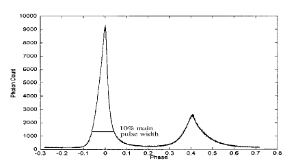
Figure 1.: The phase light curve of the Crab pulsar as taken with the fast speed photometer on board of the Hubble Space Telescope (Percival et al. 1993).

A faint 60 second periodic modulation of the Crab pulsar light curve was identified already seven years ago (Čadež & Galičič 1996) and a simple free precession model was proposed to explain the observed phenomenon (Čadež et al. 1997). We have continued to monitor the pulsar and up to the year 2001 a set of 3400 images has been built. It covers more than 20 hours of photometry data (exposure times of the images are between 4 and 15 seconds and sampling rates are between $4.0$ and $26.7$ seconds) taken with four different telescopes (the Hubble Space Telescope, the $1.22\,$m and $1.82\,$m telescopes of the Asiago Observatory and the $2.12\,$ telescope of the Guillermo Haro Observatory). Data are spanning a period of almost nine years (Čadež et al. 2001).

3. Data analysis and results

The following Fourier analysis on our data is applied to confirm for the observed 60 second modulation. For each obtained light curve $m_{k}(t_{l})$ we calculate its Fourier transform

$$F_{k}(\omega)={1\over\sqrt{2\pi(t_{l_{max}}-t_{l_{min}})}}\sum_{l}m_{k}(t_{l})~{}e^{i\omega t_{l}}~{}{{t_{l+1}-t_{l-1}}\over 2}$$ (1)

in order to test if all Fourier transforms contain a common signal at a given frequency. However, since the rotation frequency $\omega_{rot}$ of the pulsar is slowly decreasing one should expect that the free precession frequency $\omega_{fp}$ should also be decreasing. Therefore we have to allow for the recalibration of frequency scale to a common date in order to take this effect into account. The theoretical prediction (Čadež et al. 1997) is that $\omega_{fp}$ can change as $\omega_{rot}^{p}$, where p can go from 1 to 3. Thus we rescale all the Fourier transforms to the same date (Jan. 1, 1996) as

$$\tilde{F}_{k}(\omega)=F_{k}\left(\omega\left(\frac{\omega_{rot}^{\circ}}{\omega_{rot}}\right)^{p}\right)\ ,$$ (2)

where $\omega_{rot}^{\circ}$ is the pulsar’s rotation frequency at the reference date and $\omega_{rot}$ is the pulsar’s rotation frequency at the time of observations. For the value of $p$ we take 1 (Čadež et al. 2001).

With $\tilde{F}_{k}(\omega)$ we construct a matrix that has for its components cross-correlation functions between pairs of Fourier transforms

$$M_{jk}(\omega)=\tilde{F}_{j}(\omega)\tilde{F}_{k}(\omega)\ .$$ (3)

If $m_{k}$ were white statistically independent random processes, then $M_{jk}(\omega)$ for all $j$, $k$ and given $\omega$ would be a random process distributed in the complex plane according to a $2D$ Gaussian distribution. If, however, $M_{jk}(\omega)$ contain a common signal , then they are distributed in a ring around the origin of the complex plane. The probability that a common signal is present is large if the effective width of the ring is significantly smaller than its radius.

At a discrete sample of frequencies $\omega_{s}$, where $\nu_{s}=\omega_{s}/2\pi$ goes from $0.007$ Hz to $0.02$ Hz in steps of $3.3\times 10^{-4}$Hz, we calculate radial distributions $\frac{dN}{d|M_{jk}|}(\omega_{s})$ of cross-correlation functions $M_{jk}(\omega_{s})$. The number of cross-correlated pairs binned in 45 bins of width $3.3\times 10^{-4}\mathrm{mag^{2}/Hz}$ is 136 in the case of the Crab pulsar and 78 in the case of a test star. The results for the test star and the Crab pulsar are shown in Figure 2. In the case of the test star all distributions are similar which confirms the assumption of white Gaussian noise. It is apparent that the Crab pulsar is noisier than the test star which is also in agreement with Čadež et al. (2001). At a frequency $\sim 0.0167$ Hz we can see brighter colors on the contour plot for the values of $|M_{jk}|$ between 0 and 0.004 $\mathrm{mag^{2}/Hz}$ on one side and ‘a darker island’ for the values of $|M_{jk}|$ around 0.007 $\mathrm{mag^{2}/Hz}$. It is clear, that a periodic signal at the frequency $\sim 1/60\,$Hz is present.

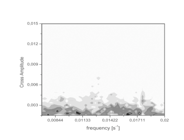
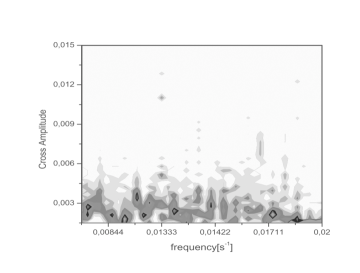
Figure 2.: Contour plot representing radial distributions of cross-correlation functions as a function of frequency for the test star (left) and the Crab pulsar (right). The x-axis represents the recalibrated frequency in Hz and y-axis represents the amplitude of the cross-correlation function in $\mathrm{mag^{2}/Hz}$. Number of $M_{jk}$ binned in 45 bins is presented with different shades of gray, the brighter is the color the lower is the number.

4. Conclusions

Presented evidence suggests that the Crab pulsar free precesses. However, the measured free precession signal is too faint to give a final answer whether the amplitude of the free precession changes with time and on what time scale the pulsar relaxes its internal stress. Examining the free precession one can learn about the equation of state of the neutron matter in pulsars. Moreover, Chandra observations of the Crab pulsar and its nebula (Weisskopf et al. 2000) has given additional motivation to understand interaction mechanisms between the pulsar and highly magnetized plasma around it. We are continuing to observe the Crab pulsar in stroboscopic mode. The increase in signal to noise ratio of the free precession signature will help answer some of the open questions regarding pulsar physics.

References

Cocke, W. J., Disney, M. J., and Taylor, D. J. 1969, Nature, Lond. 221, 525.

Čadež, A., and Galičič, M. 1996, A&A, 306, 443.

Čadež, A., Galičič, M., and Calvani, M. 1997, A&A, 324, 1005.

Čadež, A., Vidrih, S., Galičič M., and Carramiñana, A. 2001, A&A, 366, 930.

Percival, J. W., et al., 1993, ApJ, 407, 276.

Weisskopf, M. C., et al., 2000, ApJ, 536L, 81.