Optical variability of the BL Lacertae object GC 0109+224

We present the most continuous data base of optical $BVR_{c}I_{c}$ observations ever published on the BL Lacertae object GC 0109+224, collected mainly by the robotic telescope of the Perugia University Observatory in the period November 1994-February 2002. These observations have been complemented by data from the Torino Observatory, collected in the period July 1995-January 1999, and Mt. Maidanak Observatory (December 2000). GC 0109+224 showed rapid optical variations and six major outbursts were observed at the beginning and end of 1996, in fall 1998, at the beginning and at the end of 2000, and at the beginning of 2002. Fast and large-amplitude drops characterized its flux behaviour. The $R_{c}$ magnitude ranged from 13.3 (16.16 mJy) to 16.46 (0.8 mJy), with a mean value of 14.9 (3.38 mJy). In the periods where we collected multi-filter observations, we analyzed colour and spectral indexes, and the variability patterns during some flares. The long-term behaviour seems approximatively achromatic, but during some isolated outbursts we found evidence of the typical loop-like hysteresis behaviour, suggesting that rapid optical variability is dominated by non-thermal cooling of a single emitting particle population. We performed also a statistical analysis of the data, through the discrete correlation function (DCF), the structure function (SF), and the Lomb-Scargle periodogram, to identify characteristic times scales, from days to months, in the light curves, and to quantify the mode of variability. We also include the reconstruction of the historical light curve and a photometric calibration of comparison stars, to favour further extensive optical monitoring of this interesting blazar.

1 Introduction

Blazars are an extreme and rare subclass of radio-loud active galactic nuclei (AGN) showing a broad, non-thermal, polarized, and highly variable continuum flux, extending over the whole electromagnetic spectrum. The low-energy emission is likely synchrotron radiation by relativistic electrons, while the high-energy one is possibly due to Comptonization of soft photons. According to the spectral properties displayed, the subgroup of the classical BL Lacertae objects have been classified into two categories: the low-frequency peaked (LBL) and the high-frequency peaked (HBL) (e.g. Padovani & Giommi 1995; Ulrich et al. 1997). A population of intermediate BL Lacs, with the synchrotron emission peaking in the optical band, seems to link the HBL and LBL classes.

The rapid and violent optical variability is one of the defining properties of BL Lac objects. Especially the LBL and intermediate BL Lacs show large-amplitude flares, characterized by flux variations of even two orders of magnitude and covering a duration range from hours to years.

Information on variability amplitude, flux variation lags at different wavelengths, temporal duty cycles, and spectrum changes can shed light on the location, size, structure, and dynamics of the non-thermal emitting regions and on the acceleration/radiation mechanisms. A detailed knowledge of the statistical behaviour on different time scales is therefore very useful to understand the basic physical mechanisms in action during the flaring and quiescent phases. In most cases, optical data collected in the past are rather sparse and consequently not suitable to perform a detailed analysis of the blazar variability. International collaborations and robotic telescopes can improve the amount of photometric observations by one order of magnitude, so that a significant sample of these sources can be well observed and monitored in the optical band with small–medium size dedicated automatic telescopes.

In this paper we present the results of 1542 optical multiband photometric observations of the classical BL Lac objetc GC 0109+224 in the $BVR_{c}I_{c}$ Johnson-Cousins filters, during the period November 1994 – February 2002. Data were acquired mainly with the robotic telescope of the Perugia University Observatory, in Italy, joined by observations performed at the Torino Observatory, Italy, and at the Mount Maidanak Observatory, in Uzbekistan. Few Torino observations were published by Villata et al. (1997). Using these observations we analyzed the optical multiband behaviour of GC 0109+224 and investigated the type of variability on temporal scales from one day to some months.

The paper is organized as follows: in Sect. 2 we briefly review our knowledge about GC 0109+224. In Sect. 3 we describe our observing and data reduction techniques; calibration of comparison stars is presented in Sect. 4, while our $BVR_{c}I_{c}$ light curves are discussed in Sect. 5. The reconstructed historical light curve is described in Sect. 6; colour indexes are analyzed in Sect. 7, while in Sect. 8 we calculate the spectral indexes describing the variability patterns during distinct flares. In Sect. 9 we perform a statistical analysis of the data, using well-known tools for unevenly sampled time series. The summary and conclusion are outlined in Sect. 10.

2 GC 0109+224

The radio source GC 0109+224, belonging to the Green Bank Radio Survey List C (other most used names: S2 0109+22, TXS 0109+224, RX J0112.0+2244, EF B0109+2228, 2E 0109.3+2228, RGB J0112+227), was first detected in the 5 GHz Survey of the NRAO 43 m disc of Green Bank, West Virginia (Davis 1971; Pauliny-Toth et al. 1972). In 1976 this source was identified with a stellar object of magnitude 15.5 on the Palomar Sky Survey plates by Owen & Mufson (1977), who measured a strong millimeter emission (1.53 Jy at 90 GHz) and defined it as a BL Lac object.

A continuous and featureless optical spectrum was observed, for the first time, by Wills & Wills (1979). Pica (1977) recognized in GC 0109+224 an intermediate optical behaviour between the large-amplitude variability BL Lacs (e.g. BL Lac, ON 231, AO 0235+16) and the smaller-amplitude objects (e.g. ON 235, 3C 273). The host galaxy is unresolved in NTT observations (Falomo 1996) and UKIRT (K-band) observations (Wright et al. 1998). Falomo (1996) suggested a lower limit to the redshift $z\geq 0.4$ based on the optical appearance, and assuming $M_{R}=-23.5$ for it, a value similar to that characterizing some galaxies located at north-east at some arcseconds from the object. Optical spectrophotometric observations were compatible with a single power law (Falomo et al. 1994), and there was no evidence for a thermal component in the far-infrared–optical spectral energy distribution (Impey & Neugebauer 1988). Both the optical flux and the polarization are known to be variable on different timescales, including intranight variations (Sitko et al. 1985; Mead et al. 1990; Valtaoja et al. 1991). The strongly variable degree and direction of the linear polarization are one of the most noticeable characteristics of this object (Takalo 1991; Valtaoja et al. 1993). The degree of optical polarization was seen to vary between 10% and 30%, among the highest values observed in this kind of sources. There is no clear correlation between flux level and polarization. The frequency-dependence of the polarization degree is transitory, the position angle is variable and sometimes frequency-dependent (Valtaoja et al. 1993). The observed near-infrared flux variations are smaller than in the optical one (Fan 1999).

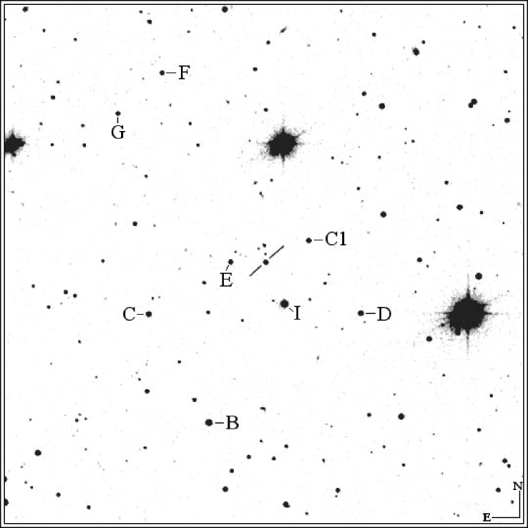
Figure 1: Finding chart with a field of 15’$\times$15’ centered on GC 0109+224 (elaborated from a frame of the Digitized Sky Survey). Calibration of stars D, C1, I, E is reported in Table 1. Stars B C F G belong to the photometric sequence calibrated by Miller et al. (1983).

Table 1: $BVR_{c}I_{c}$ Johnson-Cousins photometric calibration of comparison stars in the field of GC 0109+224.

star	R.A.	Dec.	$U^{(1)}$	$B$	$V$	$R_{c}$	$I_{c}$
	(J2000.0)	(J2000.0)	(mag)	(mag)	(mag)	(mag)	(mag)
D	01 11 53.4	+22 43 17.9	15.48	15.19 $\pm$ 0.06	14.45 $\pm$ 0.05	14.09 $\pm$ 0.05	…
C1	01 12 00.3	+22 45 22.3	…	16.30 $\pm$ 0.10	15.28 $\pm$ 0.07	14.72 $\pm$ 0.06	14.22 $\pm$ 0.08
I	01 12 03.2	+22 43 30.7	13.31	13.25 $\pm$ 0.06	12.51 $\pm$ 0.05	12.11 $\pm$ 0.04	11.76 $\pm$ 0.04
E	01 12 10.6	+22 44 40.3	15.78	16.01 $\pm$ 0.08	15.29 $\pm$ 0.07	14.94 $\pm$ 0.05	14.60 $\pm$ 0.07

• $U$ values by Miller et al. (1983)

In the radio bands the source is variable in flux, degree of polarization and position angle, showing a flat average spectrum as expected for classical BL Lacs. At the VLA milliarcsecond (pc) scale the 5 GHz radio map of GC 0109+224 reveals a compact core with a secondary component at about 3 mas at a position angle $\simeq 85^{\circ}$, with no important additional diffuse emission, and less luminous and/or beamed than the 1-Jy sample of BL Lacs (Bondi et al. 2001). The same milliarcsecond structure was evident in VLBA images at 2 and 8 GHz (Fey & Charlot 2000). The kpc scale shows a faint one-sided collimated radio jet, about 2 arcsec long, in south-western direction (Wilkinson et al. 1998), largely misaligned with the pc-scale inner region. This misalignment between structures at pc and kpc scales has frequently been observed in high-luminosity LBL. The 200-mJy sample of blazars (Marchã et al. 1996), including GC 0109+224, seems to fill the gap between HBL and LBL, as expected by unification pictures (Bondi et al. 2001). In particular, GC 0109+224 is apparently placed on the boundary between the LBL and intermediate obects. This source is regularly monitored by the University of Michigan Radio Astronomy Observatory (UMRAO), in USA, and by the Metsähovi Radio Observatory, in Finland.

It was observed in the X-ray band by HEAO-1 (Della Ceca et al. 1990), Einstein Observatory (HEAO-2, Owen et al. 1981), EXOSAT (Maraschi & Maccagni 1988, Giommi et al. 1990; Reynolds et al. 1999), and ROSAT (Neumann et al. 1994; Brinkmann et al. 1995; Kock et al. 1996, Reich et al. 2000). The source is also a member of the RGB (ROSAT All-Sky Survey-Green Bank) catalog by Laurent-Muehleisen et al. (1999), a uniform survey of classical BL Lacs generated from cross-correlating the 6 cm deep radio images with the X-ray samples. It consists in a sample of intermediate BL Lacs, with properties (like the fluxes ratio $F_{X}/F_{r}$) smoothly distributed in a large range between the LBL and HBL subclasses: for example, in the radio-optical versus optical-X spectral indexes plot, which approximately divides the HBL and LBL populations, GC 0109+224 appears close to a typical intermediate object like ON 231 (Dennett-Thorpe & Marchã 2000).

GC 0109+224 was not detected in $\gamma$-rays by EGRET (Fichtel et al. 1994), with a rather low upper limit of 0.01 nJy (above 100 MeV).

This source has recently been included in the list of blazars chosen for a project of continuous optical monitoring named the Whole Year Blazar Telescope (WYBT; Tosti et al. 2002), born from the wide international collaboration called Whole Earth Blazar Telescope (WEBT; Villata et al. 2000, 2002).

3 Observations and data reduction

The photometric observations were carried out with three instruments: the Newtonian f/5, 0.4 m, Automatic Imaging Telescope (AIT) of the Perugia University Observatory, Italy (451 meters a.s.l.), a robotic telescope equipped with a $192\times 165$ pixels CCD array, thermoelectrically cooled with Peltier elements (Tosti et al. 1996); the REOSC f/10, 1.05 m, astrometric reflector of the Torino Observatory, Italy (622 meters a.s.l.), mounting a $1242\times 1152$ pixel CCD array, cooled with liquid nitrogen and giving an image scale of $0.467^{\prime\prime}$ per pixel; the Ritchey-Chrétien f/7.74, 1.5 m, AZT-22 telescope (Novikov 1987) of the Mount Maidanak Observatory, Uzbekistan (2593 meter a.s.l.), equipped with a nitrogen cooled SITe $2048\times 800$ pixel CCD device, with a $8.5\times 3.5^{\prime}$ field of view.

The telescopes were provided with standard $UBV$ (Johnson) and $R_{c}I_{c}$ (Cousins) filters (Bessel 1979).

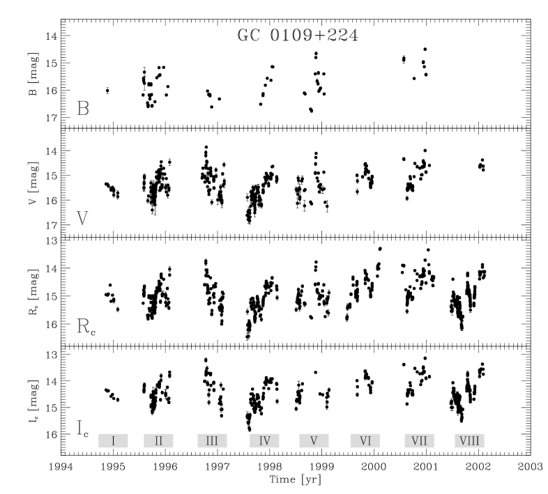
Figure 2: $BVR_{c}I_{c}$ light curves of GC 0109+224 from 1994 to 2002. All the data came from our seven-years observing campaign. The roman numbers point out the number of each observing season.

All observatories took CCD frames and performed a first automatic data reduction with batch procedures, using standard methods, to correct each raw image for dark and bias signals and to flat fielding, to recognize the field stars, and to derive instrumental magnitudes via aperture photometry or Gaussian fitting. The single frames are inspected to evaluate the quality of the image, the reliability of the data, and to search for spurious interferences. The comparison among data obtained with different telescopes in the same night reveals a good agreement, and no revealable offset was found, as already demonstrated for another source (Raiteri et al. 2001). A comparison with data in $V$ band taken in the same period at the Tuorla Observatory (Katajainen et al. 2000) revealed a good agreement.

4 Comparison stars photometry

Calibration of the source magnitude is easily obtained by differential photometry with respect to comparison stars in the same field. In order to obtain a reliable photometric sequence for GC 0109+224 we selected a set of non-variable stars with brightness comparable to the object and different colours (see the finding chart in Fig. 1). Calibrations of these stars was derived from several photometric nights at the Perugia and Torino Observatories using Landolt standards. Details on observing and data reduction procedures, filter system, and software adopted, as well as a comparison with other works can be found in Fiorucci & Tosti (1996), Fiorucci et al. (1998), Villata et al. (1998), and Raiteri et al. (1998). Data obtained by the two telescopes showed an agreement into one standard deviation, and a weighted mean on the nights number was finally adopted. The results are presented in Table 1, showing our $B,V,R_{c},I_{c}$ photometry as well as the $U$ magnitudes reported by Miller et al. (1983).

5 Optical light curves from 1994 to 2002

We have been monitoring the BL Lac object GC 0109+224 in the four $B,V,R_{c},I_{c}$ optical bands for more than 7 years, from November 12, 1994 to February 12, 2002 (JD=2449669–2452318). A total of 1542 data points was obtained in a period of 2649 days (see Fig. 2). In particular, we collected 671 photometric points in the $R_{c}$ band (the best sampled one) during eight observing seasons: the mean time lag between subsequent observations is $\Delta t=3.9$ days, the minimum lag $\Delta t=6$ minutes and the maximum lag $\Delta t=244$ days, corresponding to the interruption between the second and the third observing period.

From a direct visual inspection of the light curves structure in Fig. 2, we can identify an intermittent mode of variability, a common behaviour among BL Lacs (Tosti et al. 2001). Several moderate-amplitude outbursts are visible, together with some steep brightness drops and some periods of flickering at an intermediate level. No extraordinary big and isolated flare was detected, but six major flares are evident: at the beginning and fall of 1996, in fall 1998, at the beginning and at the end of 2000, and at the beginning of 2002.

In the third observing season (October 1996 – February 1997), an appreciable flare was detected between October and November, peaked on JD=2450367 (Oct. 11, 1996), when GC 0109+224 reached the magnitudes $V=14.08\pm 0.07$ and $R_{c}=13.75\pm 0.07$. The variability pattern of this flare is inspected in Sect. 8. The flux then dropped by almost two mag in 42 days (at JD=2450409 $R_{c}=15.63\pm 0.07$), and began to fluctuate around a low level. In the fourth observing season (July 1997 – February 1998) we observed a quasi-monotonic ascendant trend with small fluctuations on different time scales superimposed. At the end of this climbing phase the $R_{c}$ magnitude has passed from the minimum brightness value detected by us ($16.46\pm 0.13$) to $14.341\pm 0.025$. In the period October–December 1998 (in the fifth observing season), around JD=2451139 (Nov. 21, 1998) the source reached magnitudes $B=14.657\pm 0.056$ and $R_{c}=13.786\pm 0.026$, according to Torino and Perugia $BVR_{c}$ observations. A similar behaviour is observed in the sixth season (June 1999 – February 2000), where the brightness rises from an initial value of $R_{c}=15.81\pm 0.1$ at JD=2451353 to $R_{c}=13.30\pm 0.03$ (the maximum brightness observed in this band), showing at the end a prominent flare. In November–December 2000 another flare (peaking at JD=2451902 according the $B$ mag) is clearly observed by both the Mt. Maidanak and the Perugia Observatories in all $UBVR_{c}I_{c}$ filters. The variability pattern is analyzed also in this case, in detail in Sect. 8.

Figure 3: The historical light curve of GC 0109+224 in $B$ band (black dots) reconstructed from the literature (Pica 1977; Pica et al. 1980; Puschell & Stein 1980; Zekl et al. 1981; Moles et al. 1985; Pica et al. 1988; Xie et al. 1988a; Xie et al. 1988b; Mead et al. 1990; Sillanp$\ddot{\textrm{a}}\ddot{\textrm{a}}$ et al. 1991; Takalo 1991; Xie et al. 1992; Valtaoja et al. 1993; Falomo et al. 1994; Xie et al. 1994; Katajainen et al. 2000). Data after 1994 are almost entirely from this paper. $B$ magnitudes derived from $R_{c}$ values by using the mean $B-R_{c}$ index are added to improve sampling (grey circles); the maximum error for these estimates is about 0.3–0.4 mag. Pre-1960 values have original errors of 0.1 mag and represent photographic magnitudes (see text). Error bars are not represented for clarity.

The fainter and brighter magnitudes measured in the $B$ band are $16.76\pm 0.06$ (at JD=2451107, Oct 20 1998) and $14.497\pm 0.005$ (JD=2451902, Dec 23 2000) respectively, while the fainter and brighter magnitudes observed in the better sampled $R_{c}$ band are $16.46\pm 0.13$ (at JD=2450656, Jul 27 1997) and $13.30\pm 0.03$ (at JD=2451588, Feb. 13, 2000) respectively.

A general visual inspection of the light curves in Figs. 2-3 reveals the existence of a long-term oscillation of the base flux level, from which rapid flares depart.

6 The historical light curve

The optical history of GC 0109+224 extends over almost one century (1906–2002), even if there is a gap of 15 years (1960–1975) in the available data (Fig. 3). The old light curve was obtained using plates, from which a photographic magnitude $m_{pg}$ can be extracted. Recent data have been obtained directly with photoelectric or CCD photometry. A semi-empirical correction must be applied to convert $m_{pg}$ data in $B$ magnitudes. For example, one can adopt the mean shift $B=m_{pg}+0.28$, as suggested by Lü (1972), but the exact value is doubtful, due to its dependence on the variable $U-B$ index. For this reason, we chose to report the original non-corrected data, warning that pre-1961 values are overestimated in luminosity by $\sim 0.2$–0.3 mag. The optical behaviour before 1961 was reconstructed with the Heidelberg plates (Zekl et al. 1981) and the Harvard plate collection (Pica 1977). The light curve between 1976 and 1988 was mainly obtained at the University of Florida Rosemary Hill Observatory (Pica et al. 1988). The other observations are sparse literature data (see references in Fig. 3). Data after 1994 are almost entirely from this paper. To give a complete qualitative behaviour, we have reported in Fig. 3, in addition to the original $B$ magnitudes, also rough estimates of the $B$ values derived from our $R_{c}$ mag, using the mean $B-R_{c}$ color index, which is approximately constant in our period of observation (see Sect. 7).

The largest brightness variation occurred in 1942–1943, when a steep decline of 3.07 mag during one year was observed (Pica 1977), following one of the maximum values ever achieved ($m_{pg}\simeq 14.2$). A comparable brightness level was reached again only in the flares of October 1996, of November 1998, in February 2000 and in the flare of December 2000.

We also notice that from 1944 to 1996 the source was never observed brighter than $B=15$, even if this could be due to poor sampling. Variations of 0.6–0.8 mag and modest flaring were common from 1976 to 1995. In 1980 a drop of almost 2 mag made the source fainter than $B=17$, and in the period 1981–1990 the object remained in a low state around $B=17$ except for the flares of late 1981 and 1986. In particular, in August 1989 the source brightness fell down to $B=18.42$, the minimum value ever observed (Takalo 1991). In the post-1994 better sampled light curve obtained with our data, we see a general brighter mean $B$ value (15.8), again comparable with the 1920–1960 period, and some flare events. Variations of $\sim$2.5 mag in less than one year are common (a drop of 2.25 mag in 1996–97, a brightening of 2.1 mag in 1997–98 and of 2.51 mag in 1999–2000, a drop of 2.8 mag in 2001 and finally an increase of 2 mag in 2001–2002).

Figure 4: Temporal behaviour of the $I_{c}$ magnitude (upper panel) and of $V$-$I_{c}$ (middle panel) and $B$-$R_{c}$ (lower panel) colour indexes.

7 Colour indexes

Optical flux variations in BL Lacs are usually accompanied by changes in the spectral shape, and this can be revealed by analyzing color indexes. We calculated the $B-R_{c}$ and $V-I_{c}$ indexes, selecting data from the same observatory, coupling frames with a lag of no more than 15 minutes, and using only the most precise data. Since the GC 0109+224 host galaxy is faint it is reasonable to neglect the galaxy color interference in the observed flux, which instead may be important in other objects (like BL Lacertae, see e.g. Villata et al. 2002).

When plotting these two color indexes versus magnitude in different bands, we always found a certain dispersion of data around the mean values ($B-R_{c}=0.83\pm 0.08$ and $V-I_{c}=1.00\pm 0.16$). The $B-R_{c}$ index is a good indicator of reddening variations during the different variability phases, but neither solid correlations, characterized by a small dispersion of the data, nor general trends seem to be present. This means that the overall behaviour of the indexes does not depend on the source brightness.

Fig. 4 reports the long-term temporal evolution of the $V-I_{c}$ index, which appears to spread around the mean value without any noticeable trend. A larger data dispersion with larger data errors occurs when the source is faint. The less sampled $B-R_{c}$ temporal trend shows a small but clear and abrupt increase in 1996, from the mean value of 0.78 in July 1995 to the mean value of 0.94 in November 1996, meaning a spectral steppening. In the following years this color index remains nearly constant.

In the overall datasets, we found the same no-trend spreading when calculating the other color indexes and plotting them versus magnitudes. In the flares temporal windows the situation is different: a chromatic behaviour appears evident, as showed in the next section for three examples.

Table 2: The number of photometric $UBVR_{c}I_{c}$ data points of GC 0109+224 obtained by each observatory, and a summary of the data sampling and flux in each band.

NUMBER OF DATA PER OBSERVATORY

Obs.	$U$	$B$	$V$	$R_{c}$	$I_{c}$	Tot.	Period
Perugia	0	5	309	568	434	1316	Nov94-Feb02
Torino	0	56	41	96	0	193	Jul95-Jan99
Maid.	5	7	7	7	7	33	Dec00
Total	5	68	357	671	441	1542

  
  
SAMPLING AND FLUXES $B$ $V$ $R_{c}$ $I_{c}$   Start date [JD-2449000] 679 669 669 669   End date [JD-2449000] 2908 3309 3318 3309   Mean gap in data [day] 33.2 6.7 3.9 6.0   Longest time gap [day] 557 352 244 244   Mean flux [mJy] 2.39 2.88 3.38 4.47   Max flare flux [mJy] 7.85 11.66 16.16 15.10   Max/Min flux ratio 6.87 10.90 15.28 14.63   Absorption coeff. [mag] 0.161 0.124 0.100 0.073

8 Spectral indexes and variability patterns

In this section we examine possible relations between the source luminosity and the shape of the optical spectral energy distribution (SED), which can be expressed conveniently by a power law $\nu F_{\nu}\propto\nu^{-\alpha+1}$, ($\nu$ being the radiation frequency and $\alpha$ the spectral index). We have already partially investigated this with the analysis of the color indexes.

The degree of correlation between $\alpha$ and the flux sheds light on the non-thermal emitting processes, involving synchrotron and inverse-Compton cooling of a population of relativistic electrons. A common pattern, but not the unique one, during well-defined flares is the soft-hard-soft signature: the brighter the source, the harder the spectrum, in the sense that the spectral slope flattens when the source luminosity increases. This may suggest that the more intense is the energy release, the higher is the particles energy. The non-thermal acceleration mechanism tends to work with almost fixed populations of particles, in confined flaring regions in the jet.

Using data of a single telescope in at least three filters with maximum time lag of 15 minutes, we checked the degree of correlation between $\alpha$ and the flux in various bands through a least-square linear regression. Values characterized by large errors and $\chi^{2}$ were rejected. We found that the spectral index of GC 0109+224 varies between $2.23$ to $0.82$, with a mean value of $1.41\pm 0.16$.

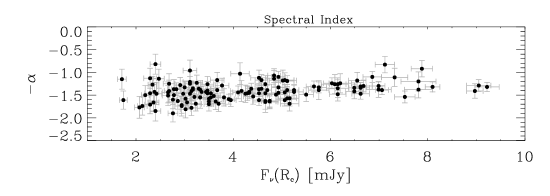
Figure 5: Spectral index $\alpha$ versus flux in the $R_{c}$ band. The linear correlation coefficient is $r_{\alpha-R}=0.29$. A weak indication of spectral flattening with brightness is recognizable (slope $0.039$).

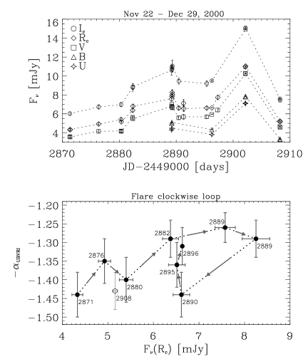
Figure 6: Evolution of the optical spectrum of GC 0109+224 as a function of the flux in the $R_{c}$ band during the double-peaked flare of November 22 – December 29, 2000. The loop formed by points connected by arrows corresponds to the first peak. In the subsequent major peak the flux achieves $F_{\nu}(R_{c})=11.04$ mJy and the spectral index $\alpha=1.09$ on day 2902 (this point is out of the plot, for clarity), and then drops rapidly to the base value $F_{\nu}(R_{c})=5.15$ mJy, $\alpha=1.39$, on day 2908 (empty circle in the plot).

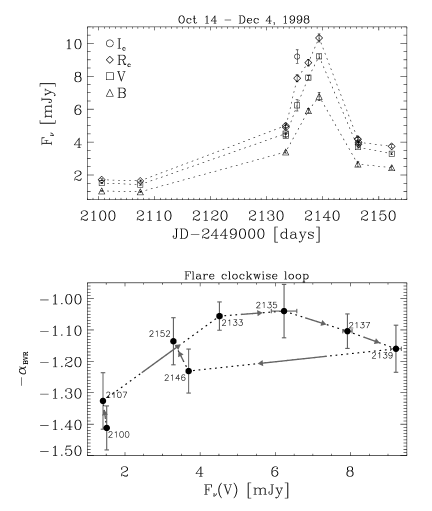
Figure 7: Evolution of the optical spectrum of GC 0109+224 as a function of the flux in the $V$ band during the isolated flare of 14 October – 4 December 1998. A well-defined clockwise loop is traced evidencing, one more time, that the spectrum gets softer when the source gets fainter.

In Fig. 5 we plotted $\alpha$ versus $R_{c}$ flux. We found correlation for the 141 data points of the Perugia Observatory, where the linear correlation coefficients for the different bands are $r_{\alpha-I}=0.18$ (pure chance probability less than 0.04), $r_{\alpha-R}=0.29$, $r_{\alpha-V}=0.36$ (chance probability 0.01), and in the 18 Torino Observatory data points, with the value $r_{\alpha-B}=0.60$ (chance probability 0.008). This increasing trend of $r$ with frequency derives from the stronger variability at higher frequency, which in turn determines the “flatter when brighter” behaviour. However, also uncorrelated random fluctuations in the emission might introduce a statistical bias due to the spectral index dependency on the flux (Massaro & Trevese 1996). An unbiased estimate of the correlation coefficient is given by the value computed for the central frequency (in this case close to that of the $R_{c}$ band), which we used as representative of the brightness state of the source. In Fig. 5 one can also notice a weak indication of spectral flattening with increasing brightness, characterized by a slope of $0.039$.

During well-defined and large flares observed in blazars at the X-ray frequencies, the spectral index versus flux shows a characteristic loop-like pattern in most cases. This is usually tracked temporally in the clockwise sense (if the power index is plotted entirely with sign). This feature is well known and has been observed for example in OJ 287 (Gear et al. 1986), PKS 2155-304 (Sembay et al. 1993; Georganopoulos & Marscher 1998; Kataoka et al. 2000), Mkn 421 (Takahashi et al. 1996), and H 0323+022 (Kohmura et al. 1994). The loops represent an hysteresis cycle in the scatter plot between the power index and the flux, and indicate that the spectrum gets steeper when the source gets fainter. They arise whenever the spectral slope is completely controlled by the radiative cooling processes, so that the information about changes in the injection rate of accelerated particles propagates from high to low energies (Kirk et al. 1998; Kirk & Mastichiadis 1999). In particular, clockwise loops mean that cooling is effective before acceleration has ceased.

In order to check the presence of this behaviour in our optical data, we selected three well-defined and strong flares of GC 0109+224, lasting less than one month. We discovered a clockwise loop from the double-peaked flare of November 22 – December 29, 2000. Fig. 6 shows that the cycle formed by the first peak is well traced by our data. From the subsequent major peak we obtained only two points, corresponding to the maximum brightness (and to the flattest spectral index) and to the minimum one, where the flux comes back to the base level from which the first peak started.

A well-defined clockwise loop comes out from the isolated flare of October 14 – December 4, 1998 (Fig. 7). The same signature of a steeper-when-dimming trend is clear.

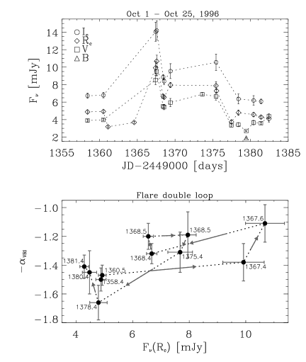
Figure 8: Evolution of the optical spectrum of GC 0109+224 as a function of the flux in the $R_{c}$ band during the double-peaked flare of October 1–25, 1996. An anticlockwise loop due to the first peak is superimposed to a second clockwise loop due to the second peak. This might be a general and nice signature of flares superimposition.

The plot obtained for the double-peaked flare lasting from October 1, 1996 to October 24, 1998 is displayed in Fig. 8. It shows an anticlockwise loop due to the first peak superimposed to a second clockwise loop due to the second peak. This could be a nice signature of the superimposition of a second flare on a previous one. The errors on $\alpha$ are large, but the data are nonetheless consistent with the discussed pattern, because of the smaller uncertainty on the flux. Anticlockwise loops are not common but have occasionally been observed (for example in the case of PKS 2155-304, Sembay et al. 1993), attesting in this case, that cooling times are comparable to acceleration times.

Our present findings show that variability loops, during isolated flares that do not blend with any preceding or subsequent variability bump, are recognizable not only in the X-ray emission, but also in the optical one, once sampling is sufficient to trace the patterns well. This suggests that during flares of the kind described above, extending over few weeks, radiative cooling dominates the spectral distribution also at the optical frequencies.

Consequently, the variations at higher frequencies (for example in the $U$ and $B$ bands) lead those at the lower frequencies (for example $R_{c}$ and $I_{c}$ bands) during both the increasing and decreasing brightness phases, reflecting the differences in the electron cooling times.

9 Statistical analysis of the time scales

In order to investigate the nature and the temporal structure of variability, the auto-correlations, the existence of characteristic time scales and possible periodicity, we applied three well-tested methods: the structure function (SF), the discrete correlation function (DCF), and the discrete Fourier transform in the Lomb-Scargle implementation (periodogram). These methods, optimized for unevenly sampled datasets, give a quantitative statistical description of the time variability.

The SF provides information on the time structure of a data train and it is able to discern the range of the characteristic time scales that contribute to the fluctuations (see e.g. Rutman 1978; Simonetti et al. 1985; Neugebauer et al. 1989; Hughes et al. 1992; Smith et al. 1993; Lainela & Valtaoja 1993; Heidt & Wagner 1996; Paltani et al. 1997, Paltani 1999). It represents a measure of the mean squared of the flux differences $(a_{i}-a_{i+\Delta t})$ of $N$ pairs with the same time separation $\Delta t$ ($a_{i}$ is the discrete signal at time $t$). We use only the first order auto-SF, defined as

$${\rm SF}^{(1)}(\Delta t)=\frac{1}{N}\sum_{i=1}^{N}\left(a_{i}-a_{i+\Delta t}\right)^{2}.$$ (1)

The general definition involves an ensemble average. For a stationary random process, the SF is related to the variance $\sigma^{2}$ and the autocorrelation function ${\rm ACF}(\Delta t)$ by ${\rm SF}^{(1)}(\Delta t)=2\sigma^{2}\left[1-{\rm ACF}(\Delta t)\right]$.

The SF is equivalent to the power spectrum, with the advantage to work in the time domain, which makes it less dependent on sampling. It removes any continue component (mean value in a period, or direct current offset) from a signal, while SF of order $n$ would remove polynomials of order $n-1$. Deep drops in the SF mean a little variance and then the signature of possible characteristic time scales.

Typically, the SF increases with $\Delta t$ in a log versus log representation, showing, in the ideal case, an initial plateau for short time lags, and a second plateau for lags longer than the maximum correlation time scale. A steep curve, whose slope depends on the fluctuations nature, links these two regions.

Figure 9: The 1994–2002 $R_{c}$ flux light curve, its structure function (data bin: 1 day, SF bin: 2 days), discrete correlation function (data bin: 1 day, DCF bin: 4 days), and periodogram ($\omega=2\pi f$). The dashed line indicates the 99% significance threshold.

The turnover time lag between the rising part and the long-lag upper flattening of the SF identifies a characteristic variability time scale of the source (Hughes et al. 1992; Lainela & Valtaoja 1993). The slope $\beta$ of the intermediate part is related to the index of the power spectral density function (PSD). A “typical” PSD has a power-law dependence on frequency $f$ in a large range: $P(f)\propto f^{-\alpha}$, where the index $\alpha$ depends on the intrinsic nature of the fluctuations. This is related to the SF slope by $\alpha=1+\beta$.

Figure 10: The II observing season (July 1995 – January 1996) $R_{c}$ flux light curve, its structure function (data bin: 1 day, SF bin: 2 days), discrete correlation function (data bin: 1 day, DCF bin: 3 days), and periodogram ($\omega=2\pi f$). The dashed line indicates the 99% significance threshold.

The DCF may be used to auto- and cross-correlate unevenly sampled data (see e.g. Edelson & Krolik 1988; Hufnagel & Bregman 1992). This function does not require any data interpolation or assumption about the light curve. The pairs $(a_{i},b_{j})$ of two discrete datasets are first combined in unbinned discrete correlations

$${\rm UDCF}_{ij}=\frac{(a_{i}-<a>)(b_{j}-<b>)}{\sigma_{a}\sigma_{b}},$$ (2)

where $<a>$ and $<b>$ are the average values of the samples and $\sigma_{a},\sigma_{b}$ their standard deviations. Each of these correlations is associated with the pairwise lag $\Delta t_{ij}=t_{j}-t_{i}$ and every value represents information about real points. The correlations (2) do not give a proper normalization if the data are noisy. The DCF is obtained by binning the ${\rm UDCF}_{ij}$ in time for each time lag $\Delta t$, and averaging over the number $M$ of pairs whose time lag $\Delta t_{ij}$ is inside $\Delta t$, i.e.: ${\rm DCF}(\Delta t)=1/M\sum_{ij}{\rm UDCF}_{ij}$. The choice of the bin size is a free parameter, and is governed by trade-off between the desired accuracy in the mean calculation, and the desired resolution in the description of the correlation curve. A preliminary time binning of data usually leads to better results, smoothing out spurious spikes; also in this case the choice of the bin size is determined by a balance between resolution and noise.

Figure 11: The IV observing season (July 1997 – February 1998) $R_{c}$ flux light curve, its structure function (data bin: 1 day, SF bin: 2 days), discrete correlation function (data bin: 1 day, DCF bin: 3 days), and periodogram ($\omega=2\pi f$). The dashed line indicates the 99% significance threshold.

The shapes of the SF and DCF reflect the nature of the process underlying the data train. Uncorrelated data produce a “white noise” behaviour, characterized by a constant PSD ($\alpha=0$). Shot noise or Brownian noise results from a sequence of random pulses, i.e. a superimposition of similar shaped bumps randomly distributed in time, with a long-term “memory”. The PSD of the standard shot noise has power law index around $\alpha=2$. Flicker noise, called also “pink noise” or $1/f^{\alpha}$ noise (with $\alpha$ approximatively in the range between 1 and 2), is an halfway between the previous two ones. This could be the result of parallel relaxation processes keeping up a certain level of memory (Ciprini et al. 2003) .

The typical BL Lac variability seems to place in between the shot and the flickering noise, even if different mechanisms could explain the rapid intrinsic flickering and the long-term flux oscillations.

Figure 12: The VIII observing season (June 2001 – February 2002) $R_{c}$ flux light curve, its structure function (data bin: 1 day, SF bin: 2 days), discrete correlation function (data bin: 1 day, DCF bin: 2 days), and periodogram ($\omega=2\pi f$). The dashed line indicates the 99% significance threshold.

Table 3: Summary of all the time scales revealed by the statistical analysis (when possible) performed with the structure function (SF), the discrete correlation function (DCF), and the Lomb-Scargle periodogram ($P(\omega)$). Columns report: (1) observing period, (2) period length, (3) time scales estimated by visual inspection, (4) time scales calculated by deep drops in the SF, (5) SF slope, (6) time scales deduced from the SF transition to the plateau, (7) time scales estimated from the DCF peaks, (8) time scales derived from the peaks of the periodogram.

Obs. period	Duration	VE $T$	SF $T_{dr}$	SF slope	SF $T_{to}$	DCF $T_{pe}$	P($\omega$) $T$
	[days]	[days]	[days]	$\beta$	[days]	[days]	[days]
1976-2002$\leavevmode\nobreak\ ({\dagger})$	26y	…	320,1.2y,1.9y,6.5y	0.55$\pm$0.06	…	340,1.2y,2.1y	1.0y,1.2y,2.0y,6.4y
1994-2002$\leavevmode\nobreak\ ({\dagger})$	7.3y	320, 1.2y	327,1.2y,1.9y	0.57$\pm$0.02	128	1.2y,1.9y	150,1.0y,1.9y
II season	186	120	12,18,74	0.68$\pm$0.06	…	13	14
III season	131	…	38,64	0.57$\pm$0.09	…	68	70
IV season	210	45	130	0.70$\pm$0.04	122	42	35, 45
V season	230	…	54	0.72$\pm$0.08	…	54	…
VI season	235	…	88	…	…	…	87
VII season	220	40	40	1.05$\pm$0.08	…	38,95	…
VIII season	235	24	26, 104	0.73$\pm$0.09	40	26,88,104	27,111

• Time scales followed by “y” are expressed in years.

An analogous technique to the Fourier analysis for discrete unevenly sampled data trains is the Lomb-Scargle periodogram $P(\omega)$, useful to detect the strength of harmonic components with a certain angular frequency $\omega=2\pi f$ (Lomb 1976; Scargle 1982; Horne & Baliunas 1986).

We applied the SF, DCF and periodogram to the historical light curve of GC 0109+224, and to each observing season of our best sampled $R_{c}$ light curve. The observed magnitude was transformed into flux density, corrected by the Galactic absorption (derived by Schlegel et al. 1998, see table 2). Fluxes relative to zero-magnitude values were taken from Bessel (1979).

A summary of the clearest statistical outcomes of our calculations is reported in Table 3: we extracted the most reliable characteristic time scales from the applied methods as well as from a preliminary visual inspection. The visual time scales are derived by identifying the repetitions of the flare peaks with similar shape, or the interval among the minima, in case we have recognized an alternating shape, or a train of successive pulses. In the time intervals where the SF slope is distinguishable in the log-log plots, we calculated its power index $\beta$ trough a linear regression.

No reliable feature was obtained from the analysis of the complete historical 1906–2002 $B$ light curve (an observational period of about 9400 days), due to the poor and very irregular sampling. In the 1976–2002 better sampled light curve, characteristic time scales of about 320 days and 1.2, 1.9, and 6.5 years are derived from SF minima, DCF peaks, and periodogram peaks. The first three time scales are confirmed by the analysis of the 1994–2002 $R_{c}$ light curve, where a significant slope of $0.57\pm 0.02$ was calculated from the SF, which shows more clearly a plateau beginning from $\Delta t=128$ days (Fig. 9). The 1.0 and 2.0 year time scales might be spurious scales due to the seasonal interruption in the sampling.

In the following we discuss briefly the single observing seasons, investigating characteristic time scales from one day to some months. Spurious correlations due to external factors are more easily avoided and the conclusions are more significant (where the sampling is sufficient) because of the lack of long empty windows among the observations and of a more regular sampling.

During the July 1995 – January 1996 period (II season, Figure 10) we revealed a SF slope of $\beta=0.68\pm 0.06$, and the DCF profile showed a clear shot noise feature, corresponding to the couple of months oscillation of the base level flux. A variability time scale of 12–14 days comes out from SF, DCF, and periodogram. In the October 1996 – February 1997 (III season), the SF did not exhibit a clear sign of a plateau. The DCF showed a central shot noise broad peak and two prominent peaks at $68$ days, confirmed by the drop in the SF and by the peak of the periodogram. In the period between July 1997 – February 1998 (IV season, Fig. 11), the SF showed a steep slope ($\beta=0.70\pm 0.04$), with hints of an upper flattening again at about 120 days. This agrees with the shot noise main component of the DCF, spreading for 120 days, and reflects the nearly monotonic rise of the underlying flux in the considered period. The periodogram shows two modest peaks corresponding to time scales of 35 and 45 days; this second value is weakly confirmed by the DCF, while the SF presents a minimum at twice this time.

During the July 1998 – February 1999 observing period (V season), a time scale of about 54 days is found. The SF slope is similar to that of the previous season. In the June 1999 – February 2000 period (VI season), a typical time scale of about 8 days comes out from a SF drop and periodogram analysis. The July 2000 – February 2001 observational window (VII season), the SF displayed a steep slope ($\beta=1.05\pm 0.09$), with no identifiable flattening. Visual inspection, SF drop, and the highest DCF peak suggest a scale of about 40 days.

In the last observing window (VIII season, June 2001 – February 2002, Figure 12) a good sampling was obtained and the characteristic time scales can be clearly extrapolated. The SF shows a slope $\beta=0.73\pm 0.10$, with a flattening at 40 days. The DCF is characterized by a central shot noise broad peak of about 40 days, with a noticeable peak at about 26 days, and minor peaks at 88 and 104 days. Such time scales are confirmed by the minima of the SF and the peaks of the periodogram.

From the above discussion and from the results summarized in Table 3, one can conclude that the light curves of the BL Lac object GC 0109+224 show indications of recurrent time scales of variability, from a dozen days to a few years. Scales of about 25–40 days and 1.2, 1.9 years were found several times, and the time scale of 6.4 years is similar to the variability period recognized in another BL Lac object: AO 0235+16 (Raiteri et al. 2001). Slopes in the SF were reliably determined, but the SF plateau can be recognized only for the best sampled light curves. The values of $\beta$ imply a variability mode between the flickering and the shot noise.

10 Summary

Seven years of optical monitoring of the BL Lac object GC 0109+224 have confirmed its intense variability. The source showed variations of about 2.5 magnitudes in less than one year, and a moderate-amplitude continuous flaring. This flaring activity appears superposed to a long-term oscillation of the base-level flux, which was recognized to vary with a time scale of about 11.6 years (Smith & Nair 1995).

The mode of variability is intermittent, characterized by relatively fast drops of the flux and by a not regular alternation of semi-quiescent and bursting phases. Our findings suggest that also in the GC 0109+224 as in other objects (like BL Lac, Villata et al. 2002) we are seeing the results of two (or maybe more) distinct mechanisms playing on different time scales. Again long-term variations seem to be essentially achromatic, while short-term flares at least in some cases follow the “flatter when brighter” feature. Indeed, when plotting the optical spectral index versus flux during three well-defined flares, clear hysteresis loops result (as usually found when analyzing the flux behaviour of BL Lacs at X-ray bands), possibly indicating that radiative cooling of a single population of accelerated electrons in a jet flaring region is dominating.

Several typical variability timescales appear from the quantitative analysis of our data, from a dozed days to a few years, but our sampling is not good enough to display any convincing evidence of periodicity. The longest characteristic time scale seen in the flux changes of GC 0109+224 is 6.5 years, very similar to the period recognized in AO 0235+16 (Raiteri et al. 2001), but poorly evident in this case. A further, continuous monitoring is required to see whether some of the time scales found in the present work are effectively linked to variability recurrent mechanisms. The optical variability of GC 0109+224 seems characterized by the $1/f^{\alpha}$ behaviour (with $1.57<\alpha<2.05$), meaning a fluctuation mode in between the flickering and the shot noise, a common feature in blazars. The power law decline of the PSD means that the frequency occurrence of a specific variation is inversely proportional to the strength of the variation. This could be caused by stochastic relaxation processes (Ciprini et al. 2003), in operation on the baseline or parsec-scale jet and generating the intermittent optical behaviour. Such intrinsic flux flickering appear then superposed to long term trends, maybe produced by external factors like jet bending.

We finally remark that the optical behaviour, the high polarization, the X-ray loudness (that could suggest a possible positive detection of $\gamma$-ray emission for the next generation of satellites like Agile and Glast), and the probable no low redshift, make GC 0109+224 an interesting BL Lac object. In this picture our data represent a useful database of the recent optical history of GC 0109+224, for future optical and multifrequency researches.

• the NASA/IPAC Extragalactic Database (NED), which is operated by the JPL-Caltech, under contract with NASA;

• Simbad Astronomical Database and Vizie-R Catalogues Services, operated at Centre de Donn es astronomiques de Strasbourg (CDS), France.

This work was partly supported by the Italian Ministry for University and Research (MURST) under grant Cofin 2001/028773.

References

- (1) Bessel, M. S. 1979, PASP, 91, 589 ARA&A, 18, 321
- (2) Brinkmann, W., Siebert, J., Reich, W., et al. 1995, A&AS, 109, 147
- (3) Bondi, M., Marchã, M. J. M., Dallacasa, D., & Stanghellini, C. 2001, MNRAS, 325, 1109
- (4) Ciprini, S., Fiorucci, M., Tosti G., & Marchili, N., 2003, in High Energy Blazar Astronomy, A. Sillanpää, L. O. Takalo & E. Valtaoja, eds., ASP Conf. Ser., in press
- (5) Davis, M. M. 1971, AJ, 76, 980
- (6) Della Ceca, R., Palumbo, G. G. C., Persic, M., et al. 1990, ApJS, 72, 471
- (7) Dennett-Thorpe, J., & Marchã, M. J. 2000, A&A, 361, 480
- (8) Edelson, R. A., & Krolik, J. H. 1988, ApJ, 333, 646
- (9) Falomo, R. 1996, MNRAS, 283, 241
- (10) Falomo, R., Scarpa, R., & Bersanelli, M. 1994, ApJS, 93, 125
- (11) Fan, J. H. 1999, astro-ph/9910269
- (12) Fey, A. L., & Charlot P. 2000, ApJS, 128, 17
- (13) Fichtel, C. E., Bertsch, D. L., Chiang, J., et al. 1994, ApJS, 94, 551
- (14) Fiorucci, M., & Tosti, G. 1996, A&AS, 116, 403
- (15) Fiorucci, M., Tosti, G., & Rizzi, N. 1998, PASP, 110, 105
- (16) Gear, W. K., Robson, E. I., & Brown, L. M. J. 1986, Nature, 324, 546
- (17) Georganopoulos, M., & Marscher, A. P. 1998, ApJ, 506, L11
- (18) Giommi, P., Barr, P., Garilli, B., Maccagni, D., & Pollock, A. M. T., 1990, ApJ, 356, 432
- (19) Gonzlez-Prez, J. N., Kidger, M. R., & Martn-Luis, F. 2001, AJ, 122, 2055
- (20) Heidt, J., & Wagner, S. J. 1996, A&A, 305, 42
- (21) Horne, J. H., & Baliunas, S. L. 1986, ApJ, 302, 757
- (22) Hufnagel, B. R., & Bregman, J. N. 1992, ApJ, 386, 473
- (23) Hughes, P. A., Aller, H. D., & Aller, M. F. 1992, ApJ, 396, 469
- (24) Impey, C. D. & Neugebauer, G. 1988, AJ, 95, 307
- (25) Katajainen, S., Takalo, L. O., Sillamp, A., et. al 2000, A&AS, 143, 357
- (26) Kataoka, J., Takahashi, T., Makino, F., Inoue, S., Madejski, G. M., et al. 2000, ApJ, 528, 243
- (27) Kirk, J. G., & Mastichiadis, A. 1999, Astropart. Phys., 11, 45
- (28) Kirk, J. G., Rieger, F. M., & Mastichiadis, A. 1998, A&A, 333, 452
- (29) Kock, A., Meisenheimer, K., Brinkmann, W., Neumann, M., & Siebert, J. 1996, A&A, 307, 745
- (30) Kohmura, Y., Makishima, K., Tashiro, M., Ohashi, T., & Urry, C. M. 1994, PASJ, 46, 131
- (31) Lainela, M., & Valtaoja, E. 1993, ApJ, 416, 485
- (32) Laurent-Muehleisen, S. A., Kollgaard, R. I., Feigelson, E. D., Brinkmann, W., & Siebert, J. 1999, ApJ, 525, 127
- (33) Lomb, N. R. 1976, Ap&SS, 39, 447
- (34) Lü, P. K. 1972, AJ, 77, 829
- (35) Maraschi, L., & Maccagni, D., 1988, MmSAIt, 59, 277
- (36) Marchã, M. J. M., Browne, I. W. A., Impey, C. D., & Smith, P. S. 1996, MNRAS, 281, 425
- (37) Massaro, E., & Trevese, D. 1996, A&A, 312, 810
- (38) Mead, A. R. G., Ballard, K. R., Brand, P. W. J. L., Hough, J. H., Brindle, C., & Bailey, J. A. 1990, A&AS, 83, 183
- (39) Miller, H. R., Mullikin, T. L., & McGimsey, B. Q. 1983, AJ, 88, 9
- (40) Moles, M., Garcia-Pelayo, J. M., Masegosa, J., & Aparicio, 1985, ApJS, 58, 255
- (41) Neugebauer, G., Soifer, B. T., Matthews, K., & Elias, J. H. 1989, AJ, 97, 957
- (42) Neumann, M., Reich, W., Fürst, E., et al. 1994, A&AS, 106, 303
- (43) Novikov, S. B. 1987, Soobshcheniya Spetsial’noj Astrofiz. Obs., 56, 23
- (44) Owen, F. N., & Mufson, S. L. 1977, AJ, 82, 776
- (45) Owen, F. N., Helfand, D. J., & Spangler, S. R. 1981, ApJ, 250, 550
- (46) Padovani, P., & Giommi, P. 1995, ApJ, 444, 567
- (47) Pauliny-Toth, I. I. K., Kellermann, K. I., Davis, M. M., Fomalont, E. B., & Shaffer, D. B. 1972, AJ, 77, 265
- (48) Paltani, S. 1999, PASPC, 159, 293
- (49) Paltani, S., Courvoisier, T. J.-L., Blecha, A., & Bratschi, P. 1997, A&A, 327, 539
- (50) Pica, A. J. 1977, AJ, 82, 935
- (51) Pica, A. J., Pollock, J. T., Smith, A. G., et al. 1980, AJ, 85, 1442
- (52) Pica, A. J., Smith, A. G., Webb, J. R., et al. 1988, AJ, 96, 1215
- (53) Press, W. H., & Rybicki, G. B. 1989, ApJ, 338, 277
- (54) Puschell, J. J., & Stein, W. A. 1980, ApJ, 237, 331
- (55) Raiteri, C. M., Villata, M., Aller, et al. 2001, A&A, 377, 396
- (56) Raiteri, C. M., Villata, M., Lanteri, L., Cavallone, M., & Sobrito, G. 1998, A&AS, 130, 495
- (57) Reich, W., Fuerst, E., Reich, P., et al. 2000, A&A, 363, 141
- (58) Reynolds, A. P., Parmar, A. N., Hakala, P. J., et al. 1999, A&AS, 134, 287
- (59) Rutman, J. 1978, Proc. IEEE, 66, 1048
- (60) Scargle, J. D. 1982, ApJ, 263, 835
- (61) Schlegel, D. J., Finkbeiner, D. P., & Davis, M. 1998, ApJ, 500, 525
- (62) Sembay, S., Warwick, R. S., Urry, C. M., Sokoloski, J., George, I. M., et al. 1993, ApJ, 404, 112
- (63) Sillanp, A., Mikkola, S., & Valtaoja, L. 1991, A&AS, 88, 225
- (64) Simonetti, J. H., Cordes, J. M., & Heeschen, D. S. 1985, ApJ, 296, 46
- (65) Sitko, M. L., Schmidt, G. D., & Stein, W. A. 1985, ApJS, 59, 323
- (66) Smith, A. G., & Nair, A. D. 1995, PASP, 107, 863
- (67) Smith, A. G., Nair, A. D., Leacock, R. J., & Clements, S. D. 1993, AJ, 105, 437
- (68) Takalo, L. O. 1991, A&AS, 90, 161
- (69) Takahashi, T., Tashiro, M., Madejski, G., Kubo, H., Kamae, T., et al. 1996, ApJ, 470, L89
- (70) Tosti G., Villata M., & Carini, M., et al. 2002, in Blazar Astrophysics with BeppoSAX and Other Obs., ASI Special Pub., ed. P. Giommi, E. Massaro, & G. Palumbo, ESA-ESRIN Rome, p. 285
- (71) Tosti, G., Ciprini, S., Massaro, E., et al. 2001, in AIP Conf. Proc. 588, High Energy Gamma-Ray Astronomy, ed. F. A. Aharonian & H. J. Völk, p. 728
- (72) Tosti, G,, Pascolini, S., & Fiorucci, M. 1996, PASP, 108, 706
- (73) Ulrich, M.-H., Maraschi, L., & Urry, C. M., 1997, ARA&A, 35, 445
- (74) Valtaoja, L., Karttunen, H., Efimov, Y. S., & Shakhovskoy, N. M. 1993, A&A, 278, 371
- (75) Valtaoja, L., Sillanpää, A., Valtaoja, E., Shakhovskoi, N. M., & Efimov, I. S. 1991, AJ, 101, 78
- (76) Villata, M., Raiteri, C. M., Ghisellini, G., De Francesco, G., Bosio, S. et al. 1997, A&AS, 121, 119
- (77) Villata, M., Raiteri, C. M., Lanteri, L., Sobrito, G., Cavallone, M. 1998, A&AS, 130, 305
- (78) Villata, M., Raiteri, C. M., Kurtanidze, O. M., Nikolashvili, M. G., Ibrahimov, M. A. et al. 2002, A&A, 390, 407
- (79) Villata, M., Mattox, J. R., Massaro, E., Nesci, R., Catalano, S. et al. 2000, A&A, 363, 108
- (80) Wilkinson, P. N., Browne, I. W. A., Patnaik, A. R., Wrobel, J. M., & Sorathia, B. 1998, MNRAS, 300, 790
- (81) Wills, B. J., & Wills, D. 1979, ApJS, 41, 689
- (82) Wright, S. C., McHardy, I. M., Abraham, R. G., et al. 1998, MNRAS, 296, 961
- (83) Xie, G. Z., Lu, R. W., Zhou, Y., et al. 1988a, A&AS, 72, 163
- (84) Xie, G. Z., Li, K. H., Zhou, Y., et al. 1998b, AJ, 96, 24
- (85) Xie, G. Z., Li, K. H., Liu, F. K., et. al. 1992, ApJS, 80, 683
- (86) Xie, G. Z., Li, K. H., Zhang, Y. H., et al. 1994, A&AS, 106, 361
- (87) Zekl, H., Klare, G., & Appenzeller, I. 1981, A&A, 103, 342