Are Chaplygin gases serious contenders to the dark energy throne?

Abstract

We study the implications on both background and perturbation evolution of introducing a Chaplygin gas component in the universe’s ingredients. We perform likelihood analyses using wide-ranging, SN1a, CMB and large scale structure observations to assess whether such a component could be a genuine alternative to a cosmological constant, $\Lambda$. We find that the current data favors behavior in an adiabatic Chaplygin Gas that is akin to a cosmological constant.

I Introduction

Supernovae observations super1 ; superP first indicated that the universe’s expansion has started to accelerate during recent cosmological times. This, and further observations, e.g. of the Cosmological Microwave Background (CMB) or Large Scale Structures (LSS) , suggest that the energy density of the universe is dominated by a dark energy component, with a negative pressure, driving the acceleration. One of the substantive goals for cosmology, and for fundamental physics, is ascertaining the nature of this dark energy. Maybe the most attractive option would be a cosmological constant, $\Lambda$, however there are infamous fine-tuning and coincidence problems associated with explaining why $\Lambda$ should have today’s energy scale. These problems have lead to a wealth of dynamical, scalar, dark energy (“quintessence”) models being proposed as alternatives to $\Lambda$ (see Peebles02 for a good review). Even in these cases, however, explaining why our epoch should be so crucial in triggering the acceleration still requires fine-tuning.

A concurrent problem is the nature of the non-baryonic, clumping dark matter component required in the standard model to give Large Scale Structure predictions consistent with observations.

Recently an alternative matter candidate, a Generalized Chaplygin Gas (GCG), has been proposed as a potential ‘hybrid’ solution to both the dark energy and dark matter problems. The GCG can be seen to evolve in a wide range of contexts, for example from supersymmetry, tachyon cosmologies Gibbons03 and brane cosmologies Bilic01 . A recent letter Teg02 dealt with the implications for the matter power spectrum in the absence of CDM and effectively ruled out the GCG as a CDM substitute.

In this paper we investigate the strength of the GCG as a dark energy candidate. Although there have been a number of papers discussing various aspects of GCG behavior (Kamen01 -Gonz02 ) there has not been, as yet, a full analysis of the constraints that can be placed on such models from the wide range of complementary data sets currently available. This is necessary if such exotic matter types are to be considered as serious alternatives to the $\Lambda$-CDM scenario.

In section II we review the background evolution of the GCG and discuss the implications for supernovae (SN1a) observations. Although such constraints are important, a wide range of proposed theories can generate the required expansion profile (see Peebles02 for dark energy theories and, for example, Deffayet02 for an alternative to dark energy). In order to better discriminate between theories, perturbation dependent observables must be taken into consideration. In section III we extend our discussion to perturbations in the Chaplygin gas and discuss the implications for structure formation in the presence of an adiabatic Chaplygin fluid. In section IV we consider the effects on radiation perturbations and the CMB spectrum. In section V we present the main results of the paper, likelihood analyses for a CDM+GCG+baryon universe. We include the option of a pure GCG + baryon scenario ($\Omega_{c}=0$) for completeness. We obtain a clear indication of the strength of the GCG model when compared to CDM and $\Lambda$. In section VI we summarize our findings and assess the true potential of Chaplygin gases as a dark energy contender.

II Background evolution

The Generalized Chaplygin models can be characterized by three parameters: $w_{0}$, $\alpha$ and $\Omega_{ch}^{0}$. The equation of state nowadays $w(a=1)=-|w_{0}|$ and the index $\alpha$ specify the equation of state evolution,

$$p=-{|w_{0}|\Omega_{ch}^{0}\rho_{0}\over\rho^{\alpha}}.$$ (1)

where $\rho_{0}=3H_{0}^{2}$ $(8\pi G=1)$ is the total energy density today. The energy conservation equation, $\dot{\rho}+3{\cal H}(1+w)\rho=0$, admits a solution for $\rho(a)$ specified by $|w_{0}|$, $\alpha$ and the fractional energy density today, $\Omega_{ch}^{0}$,

$$\rho(a)=\Omega_{ch}^{0}\rho_{0}\left[|w_{0}|+{(1-|w_{0}|)\over a^{3(1+\alpha)}}\right]^{{1\over 1+\alpha}}$$ (2)

. The equation of state then evolves as,

$$w(a)=-{|w_{0}|\over\left[|w_{0}|+{(1-|w_{0}|)\over a^{3(1+\alpha)}}\right]}.$$ (3)

At early times the GCG’s equation of state tends to zero, mimicing CDM . The value of $\alpha$ determines the redshift of transition between the two asymptotic behaviors; the greater the value of $\alpha$ the lower the transition redshift. At early times, the total amount of matter with $w\sim 0$ reaches an asymptotic value

$$\Omega_{m,eff}^{0}=\Omega_{m}^{0}+\Omega_{ch}^{0}\left(1-|w_{0}|\right)^{{1\over 1+\alpha}}$$ (4)

where $\Omega_{m}$ is the baryonic + CDM density fraction. Note that the unique ability of the GCG to account for both the dark energy like behavior at late times and for ordinary dark matter at early times motivated the original studies of this particular equation of state.

In previous discussions $\alpha$ has often been assigned a positive value in the range $0<\alpha<1$, in order to be consistent with various higher dimensional theories that can produce a perfect fluid stress-energy tensor satisfying the criterion in (1) (see for example Podolsky02 ). In our study, we extend the range of values of $\alpha$ considered to $-1<\alpha<\infty$ in order to obtain a broader assessment of whether Chaplygin gases could be a viable alternative to the standard model.

For $\alpha$=0 the background evolution of the Chaplygin gas is identical to a $\Lambda$-CDM model with $\Omega_{\Lambda,eff}=\Omega_{ch}|w_{0}|$, and $\Omega_{m,eff}=\Omega_{m}+\Omega_{ch}(1-|w_{0}|)$. Furthermore, as is visible in equations (2) and (3), when $|w_{0}|$ tends to 1, the GCG component tends to evolve as a cosmological constant, irrespective of the value of $\alpha$. Note that there is no analogous quintessence like behavior (with $w_{0}\neq-1$), thus we are only comparing GCG to theories including $\Lambda$.

Figure 1: Contours in $\Omega_{ch}-|w_{0}|$ space with the same luminosity distance as a fiducial model $\Lambda$-CDM model with $\Omega_{\Lambda}=0.7$ at $z=0.5$ (top) and $z=1$ (bottom). For $\alpha=0$ (full line) the luminosity distance curve is identical to that of the fiducial model at all redshifts.

The SN1a observations measure the apparent magnitude, $m(z)$, related to the luminosity distance, $d_{L}(z)$ via,

$$m(z) = {\cal M}+5\log{d_{L}(z)}+25,$$ (5)

$$d_{L} = (1+z)\int_{0}^{z}{dz^{\prime}\over H(z^{\prime})}$$ (6)

where $\cal{M}$ is the absolute bolumetric magnitude and $d_{L}$ is measured in Mpc. It is easy to see that, because the background evolution (through $H$) wholly determines luminosity distance predictions, the degeneracy between a GCG with $\alpha=0$ and $\Lambda$-CDM will allow the Chaplygin gas to fit the SN1a data well. Indeed the degeneracy also stretches to $\alpha\neq 0$ when one considers luminosity distance at a specific redshift. In figure 1 we show Chaplygin models with degenerate luminosity distances with a fiducial $\Lambda$-CDM model with $\Omega_{\Lambda}$=0.7, at $z=0.5$ and 1.0. This degeneracy, however, implies that the SN1a observations cannot be a strong discriminant between the GCG and $\Lambda$; we must look to alternative, perturbation-dependent observations to test the validity of the GCG models.

III Chaplygin gas perturbations

We treat the Chaplygin gas as a perfect fluid made up of effectively massless particles interacting with the rest of matter purely through gravity. We assume purely adiabatic contributions to the perturbations so that the speed of sound for the fluid is

$$c_{s}^{2}={\delta p\over\delta\rho}={\dot{p}\over\dot{\rho}}=-w\alpha$$ (7)

and the time variation of $w$ is

$$\dot{w}=-3{\cal H}\left(1+w\right)\left(c_{s}^{2}-w\right)=3{\cal H}w(1+w)(\alpha+1)$$ (8)

where derivatives are with respect to conformal time (d/d$\tau$), and $a{\cal H}=da/d\tau$.

Figure 2: Late-time $\delta$ evolution as a function of $\alpha$ and $|w_{0}|$ for 4 scales $k/{\cal H}$ = 1,10,100,1000 (${\cal H}\approx 3000hMpc^{-1},h=0.65$). Regions [1] and [2] undergo power law growth and decay respectively and [3] undergoes oscillatory decay.

In the synchronous gauge and following the approach and notations of Ma and Bertschinger Ma95 , we can write down the evolution equations for the density and velocity divergence perturbations, $\delta$ and $\theta$, using the conservation of energy momentum tensor $T^{\mu}_{\nu;\mu}=0$,

$$\dot{\delta} = -\left(1+w\right)\left(\theta+{\dot{h}\over 2}\right)-3{\cal H}\left(c_{s}^{2}-w\right)\delta,$$ (9)

$$\dot{\theta} = -{\cal H}\left(1-3c_{s}^{2}\right)\theta+{c_{s}^{2}\over(1+w)}k^{2}\delta-k^{2}\sigma.$$ (10)

The fluid is highly non-relativistic and therefore we assume the shear perturbation $\sigma=0$.

At early times, when the Chaplygin gas has $w\approx 0$, the GCG perturbations evolve like those of ordinary dust with $\dot{\theta}=\theta=0$, and $\dot{\delta}=-\dot{h}/2$. In the radiation era $\delta(a)\propto a^{2}$ , while $\delta\propto a$ in the early GCG dominated era. At later times, when the GCG’s equation of state starts to decrease, the perturbations stray drastically from this dust-like evolution.

We can understand the late-time behavior more clearly if we evaluate the second order differential equation for $\delta$. By differentiating equation (9) with respect to time we find, as outlined in an appendix (section VII), for a general, shearless, fluid,

$$\ddot{\delta} + \left[1+6(c_{s}^{2}-w)\right]{\cal H}\dot{\delta}$$ (11)

$$+ \left[9{\cal H}^{2}(c_{s}^{2}-w)^{2}+3{\cal H}(\dot{c_{s}^{2}}-\dot{w})+3{\ddot{a}\over a}(c_{s}^{2}-w)+c_{s}^{2}k^{2}\right]\delta$$

$$=-3c_{s}^{2}(1+w){\cal H}\theta+{a^{2}\over 2}(1+w)(3\delta P+\delta\rho).$$

Figure 3: Late time evolution envelope for $\delta$. The power, $n_{eff}=\tau\dot{\delta}/\delta$, is plotted for two length scales $k/{\cal H}$ = 10 and 100. In the oscillatory regime $n_{eff}$ for the bounding envelope is plotted.

Numerical integration shows that the coupling to $\theta$ in equation (11) is subdominant for all scales that we are interested. For the Chaplygin gas,

$$\ddot{\delta} + A{\cal H}\dot{\delta}+B{\cal H}^{2}\delta-{3{\cal H}^{2}\over 2}(1+w)\Omega_{c}\delta_{c}=0,$$ (12)

$$A = 1-6w(\alpha+1),$$ (13)

$$B = -{3{\cal H}^{2}\over 2}\left\{\Omega_{ch}+\left[7+\Omega_{ch}+(13-3\Omega_{ch})\alpha+6\alpha^{2}\right]w\right.$$ (14)

$$\left.-3\Omega_{ch}(1+2\alpha)w^{2}+{2\alpha w\over 3}\left({k\over{\cal H}}\right)^{2}\right\},$$

where the subscript $c$ refers to cold dark matter.

For $w=0$, (12) reduces to the expected, scale independent, CDM evolution with $\delta\propto\tau^{2}$. For $w\neq 0$ we retain scale independence if $\alpha=0$ and just get suppression of density perturbations. However for $\alpha\neq 0$ the perturbation evolution becomes scale dependent with the $(k/{\cal H})^{2}$ term dominating the others for scales greater than a characteristic scale

$$k_{*}^{2}={{\cal H}^{2}\over|\alpha w|}.$$ (15)

There are 3 possible solution types, for $k\gg k_{*}$,

$$\begin{array}[]{cll}\textrm{[1]}:&\textrm{growing\ mode},&\alpha<0,\\ \textrm{[2]}:&\textrm{decaying\ mode},&\alpha\sim 0,\\ \textrm{[3]}:&\textrm{oscillatory decay},&\alpha>0.\end{array}$$ (16)

In figure 2 we show the asymptotic behavior at late times (taking $w\approx-|w_{0}|$) as one increases the scale $k/{\cal H}$. In figure 3 we show the associated scaling of $\delta$, plotting $n_{eff}=\tau\dot{\delta}/\delta$. For $|w_{0}|\neq 0$, and $\alpha>0(<0)$ GCG perturbations are suppressed (promoted) in comparison to those for a $\Lambda$-CDM model.

The GCG also has an effect on the the CDM perturbations through the relation:

$$\ddot{\delta}_{c} + {\cal H}\dot{\delta}_{c}-{3{\cal H}^{2}\over 2}\left[\Omega_{c}\delta_{c}+(1-3\alpha w)\Omega_{ch}\delta\right]=0.$$ (17)

If $|w_{0}|\neq 0$ and $\alpha>0(<0)$ the GCG drives suppression (growth) in $\delta_{c}$. In figure 4 we show the power law evolution of $\delta_{c}$, plotting $n_{eff,c}=\tau\dot{\delta}_{c}/\delta_{c}$ for 3 scales as one varies $\alpha$. The strong growth in $\delta_{c}$ effectively rules out a GCG with $\alpha<0$ as a dark energy candidate.

Note that the $\alpha$=0 degeneracy present in the background evolution is not found in the perturbations. The matter power spectrum and CMB spectrum will therefore be better discriminators between $\Lambda$ and the GCG than SN1a.

Figure 4: Evolution of $n_{eff,c}=\tau\dot{\delta_{c}}/\delta_{c}$ for $|w_{0}|=0.5$ and $\alpha$=-0.1 (short dash), 0 (long dash), 0.1 (long-short dash), 0.5 (dot dash) in comparison to pure CDM model (full line). Three length scales $k=10^{-4},10^{-2},10^{-1}hMpc^{-1}$ are considered.

IV Implications for temperature anisotropies

A Chaplygin gas matter component would change the temperature anisotropy specturm in a number of ways; altering the late-time ISW effect, the peak positions and relative heights.

The GCG’s late-time evolution will alter the evolution of the gravitational potential the CMB photons pass through to reach us, inducing an ISW effect. Following Seljak96 and again using the terminology of Ma95 , the ISW temperature anisotropy is given by a source,

$$S_{ISW} \propto -\dot{\Psi}+\dot{\Phi}$$

$$\propto {d\over d\tau}\left[-{3\over 2}(\rho+P)a^{2}\sigma-a^{2}\delta\rho-3{\cal H}a^{2}(\rho+P){\theta\over k^{2}}\right]$$

where $\Phi$ and $\Psi$ are the Bardeen variables Bardeen .

Figure 5: Large scale ISW effect for GCG with $\alpha$=-0.5 (long dash), 0 (short dash-dot) and 1 (long dash -dot) compared against a CDM+baryon (short dash) and ‘fiducial’ $\Omega_{\Lambda}=0.7,\Omega_{m}=0.3$ (full line) models.

At late times the shear, $\sigma$, is negligible and it is the density perturbation that drives the ISW effect.

$${d\over d\tau}\left[-{a^{2}\delta\rho}\right] \sim a^{2}\left[(1+3w)-{n_{eff}\over p}\right]{{\cal H}\rho\delta}$$ (19)

where $n_{eff}$ is the power law index and $p={\cal H}\tau$ as described in section III. Equation (19) shows why in a standard CDM scenario, with $w=0$ and $n_{eff}$ and $p$ both $\approx 2$, there is no appreciable ISW effect. In section III however we saw for $\alpha<0$ that $n_{eff}>2$ giving a negative ISW effect, while for $\alpha>0$, $n_{eff}<2$ producing an increase in the ISW temperature anisotropy. These effects are shown in figure 5.

The position of the first peak will be altered through adjustments to the sound horizon, $r_{shor}$, and angular diameter distance at the last scattering surface, $d_{A}$. The position of the first peak in multipole space is given by

$$l_{A}={\pi d_{A}(z_{rec})\over r_{shor}(z_{rec})}$$ (20)

with

$$d_{A} = \tau_{0}-\tau_{rec}$$

$$\approx {1\over H_{0}}\int^{1}_{a_{rec}}{da\over\left[\Omega_{m}^{0}a+\Omega_{ch}^{0}a^{4}(|w_{0}|-{1-|w_{0}|\over a^{3(1+\alpha)}})^{1\over 1+\alpha}\right]^{1\over 2}}$$

$$r_{shor} = \int_{0}^{\tau_{rec}}c_{s}^{\gamma b}d\tau$$

$$\approx {1\over H_{0}\sqrt{\Omega_{m,eff}^{0}}}\int_{0}^{a_{rec}}{c_{s}^{\gamma b}da\over a^{{1\over 2}}}$$

where $\Omega_{m,eff}^{0}$ is defined in equation (4) and $c_{s}^{\gamma b}$ is the speed of sound for the radiation-baryon system, not to be confused with $c_{s}$ for the Chaplygin gas (at this time the Chaplygin gas is behaving like dust and has $c_{s}^{2}=0$). For fixed $\omega_{b}=\Omega_{b}h^{2}$ and $\omega_{c}=\Omega_{c}h^{2}(h=H_{0}/100)$, $l_{A}$ increases as one increases $\alpha$ or $|w_{0}|$. The position of the first peak would be the same for scenarios with the same value of $\sqrt{\Omega_{m,eff}^{0}}d_{A}$.

Figure 6: Comparison of CMB power spectra, normalized to COBE at $l=10$, with varying $\alpha$ and $|w_{0}|$, keeping all other relevant quantities fixed. The behavior of peak heights and positions is discussed in the text.

Because the Chaplygin gas mimics matter at early times there is no simple degeneracy, governed by the peak positions, as there is for quintessence models (see for example Bean01 ). The peak heights, when compared to the low $l$ ‘plateau’, depend upon $\alpha$ and $|w_{0}|$ through their influence on the ISW effect, the horizon scale at matter-radiation equality, $l_{eq}$, (through $\Omega_{m,eff}^{0}h^{2}$) and the depth of the potential well at last scattering (also through $\Omega_{m,eff}^{0}h^{2}$).

We follow the phenomenological discussion in Hu01 , to predict how the peak heights will alter for fixed $\omega_{b}$ and $\omega_{c}$. Increasing $\alpha$, increases $\Omega_{m,eff}^{0}$, so that matter-radiation equality happens earlier, increasing $l_{eq}$ and curtailing the driving effect that the decay of the gravitational potential has on $\delta_{\gamma}$ oscillations during the radiation era. This lowers the height of the first peak, a decrease which is compounded by the raising of the plateau from the ISW effect. An earlier matter-radiation equality also decreases the depth of the potential well at last scattering, which combined with the reduction in radiation driving, increases the height of the third peak in comparison to the first and second ones.

As one increases $|w_{0}|$ one decreases $\Omega^{0}_{m,eff}$, lowering $l_{eq}$, and increasing the height of the first peak. This is tempered, however, by the increase in plateau height from the ISW effect. Reducing $l_{eq}$ acts to decrease the height of the third peak in comparison to the second and first ones. These behaviors are confirmed by the full analysis, as is shown in figure 6.

The multitudinous effects that the GCG has on the CMB spectrum make comparison with CMB observations a strong test for the GCG models as will be seen below.

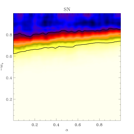
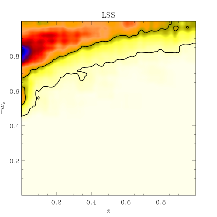
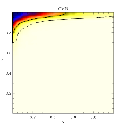
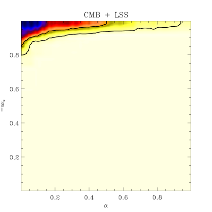
Figure 7: Joint posterior of the $\alpha$ and $-w_{0}$ parameters considering only SN1a data (top-left panel), LSS data (top-right panel), CMB data (bottom-left) and jointly CMB and LSS data (bottom-right). The contours represent the subsequent 68% and 95% confidence regions. While SN1a data induce constraints that are quite loose, LSS and CMB constraints are much tighter and tend to favor a cosmological constant like scenario.

V Chaplygin gas likelihood analysis

In order now to assess the viability of a GCG+CDM+baryon universe, we turn to evaluate the probability (the posterior) of these models given some current observations, namely SN1a, CMB and LSS probed through galaxy survey.

To study the posterior distribution, we use the Baye’s theorem and rewrite it as the product of the likelihood and the prior (we assume the evidence is constant and thus ignore it). To probe this posterior, we consequently compute both the likelihood and the prior at various positions in the chosen restricted parameter space. This sampling is conducted via the construction of a Monte Carlo Markov Chain through the Metropolis-Hasting algorithm. Once converged, this chain provides us with a collection of independant samples from the posterior (see ChMe00 ; ChMe01 ; MCMC for an introduction to this technique in this context and ChGr95 ; Gil96 for general guidance).

Our code uses some likelihood computation elements from the code described in MCMC , and relies on a version of the CAMB code CAMB extended to include a Chaplygin gas component in order to calculate CMB power spectra and matter power spectra. As input data, we considered the apparent magnitudes of 51 Supernovae superP , CMB data sets from COBE COBE , MAXIMA MAX , BOOMERANG Boom , and VSA VSA and large scale structure data from 2dF 2dF . We consider only flat models, i.e. $\Omega_{K}=0$ with scale invariant initial power spectrum, i.e. $n_{s}=1$. We use stringent (Gaussian) priors on $H_{0}$ using the HST Key Project results $h=0.72\pm 0.08$ HST and on $\omega_{b}=\Omega_{b}h^{2}=0.02\pm 0.001$ using BBN constraints BBN .

We normalize the matter power spectrum using $A_{s}$, the initial power spectrum normalization, and following Hamilton92 , we use $\beta$ and $b_{1}$ to parameterize redshift-space distortions and (linear) bias respectively. The power spectrum is then related to the transfer function $T(k)$ (computed with CAMB) by

$$P(k)=A_{s}\left(1+{2\beta\over 3}+{\beta^{2}\over 5}\right)b^{2}_{1}T(k)^{2}.$$ (23)

In order to alleviate the natural degeneracy between $A_{s}$ and $b_{1}$ (as far as LSS constraints are concerned), we use the 2dF results Peacock01 ; Verde02 to impose strong (Gaussian) priors on $\beta$ and $b_{1}$, i.e. $\beta=0.54\pm 0.09,b_{1}=1.04\pm 0.11$.

Throughout this analysis, we ensured the chains’ convergence by generating and comparing several of them (typically containing $~{}10^{5}$ elements) and by checking the so-called “parameter mixing” amid them. After several trials, we choose the proposal density for each parameter to be a Gaussian whose width is close to the final one and whose center is the last chain values. This allows a full exploration of the parameter space. To pick-up the next chain element, we allow only 1 to 3 directions (this number is randomly chosen) to vary. This gives us an acceptance rate around 25%, a good target value for efficiency’s sake Gil96 . The first 4000 elements of the chain, prior to its convergence, are thrown away and no extra thinning is applied Gil96 .

Once converged, the chains provide a fair sampling of the full posterior distribution so that we can deduce easily from it all the quantities of interest, e.g. the (joint) marginalized distribution of any parameter(s).

As stated above, we are interested in finding the compatibility of a Chaplygin gas + CDM + baryon universe with current data. For this we vary only 8 parameters $\{h,\omega_{b},\omega_{cdm},\alpha,w_{0},b,\beta,A_{s}\}$ and impose the priors stated above. We allow a free proposal distribution for $\omega_{c}$, including $\omega_{c}=0$ consistent with a unified matter universe purely containing a GCG and baryons. This allows the full breadth of GCG roles (as both a dark matter and dark energy candidate) to be tested. Following section III’s discussion, we restrict ourselves to $0\leq\alpha\leq 1$ and $-1\leq w_{0}\leq 0$. In figure 7 we plot the marginalized joint distribution of the $\alpha$, $|w_{0}|$ parameters (which is in this case just the joint number density of those parameters), as well as the 68% and 95% confidence contours, considering separately SN1a, LSS, CMB data sets, and also jointly CMB and LSS. Note that for visual purposes only the displayed surface has been build by oversampling our samples using cubic interpolation. This does not affect the quantitative interpretation since the distributions turn out to be smooth.

The interpretation of the contours is nicely consistent with the theoretical prospects discussed above. First, the SN1a observations (top-left panel) offer very light constraints on the GCG parameters, since they are sensitive only to the background evolution. Any $\alpha$ value appear viable, extending thus the obvious degeneracy between $\Lambda$-CDM model and GCG models with $\alpha=0$ discussed in section II (e.g. see figure 1). As soon as density perturbations are considered, the constraints tighten drastically. For both LSS and CMB, the isocontours are roughly centered on the $\alpha=0$, $w_{0}=-1$ model, that corresponds to the GCG acting like a $\Lambda$ term. This fact is emphasized in the joint CMB + LSS analysis. Note that in the limit that $w_{0}$ tends to $-1$ (we however impose $|w_{0}|<1$), the GCG component tends to behave like a $\Lambda$ term, irrespective of the precise value of $\alpha$, thus leading to the observed degeneracy in the $-w_{0}=1$ direction.

The other varied parameters, i.e. $h$, $\omega_{b}$ and $\omega_{cdm}$, as well as the flatness imposed $\Omega_{c}h$, exhibit (joint) distributions similar to those found in typical $\Lambda$-CDM model studies (see e.g. MCMC ). This leads us to the the main conclusion of this study: the current data tends to favor ordinary $\Lambda$ theory. When marginalized over all other parameters, we indeed find, $\alpha<0.5,0.93$, and $w_{0}<-0.85,-0.8$, both respectively at the 68% and 95% confidence level.

VI Conclusions

We have investigated the effect of a Chaplygin gas matter component in the universe’s ingredients, to see if such a component is consistent with observations and whether it is a feasible alternative to CDM and $\Lambda$.

Through inherent degeneracies with $\Lambda$ in the background evolution, the Chaplygin gas models have a good fit with SN1a data. These degeneracies are not present, however, in the perturbation evolution. In particular the growth/suppression of both GCG and CDM density perturbations proves distinctive when comparing against large scale structure observations; this statement is valid, of course, for all cases (for all $\alpha$) except, naturally, $w_{0}-=-1$ which is identical to $\Lambda$, and has no perturbations. The GCG also introduces a number of distinguishing differences from the $\Lambda$-CDM CMB spectrum through altering the potential at last scattering, the ISW signature, the equality scale, and the angular diameter distance to last scattering. Combined, these differences provide a strong test for the GCG scenario.

We performed likelihood analyses using SN1a, CMB and LSS datasets and found that the current data strongly prefers a $\Lambda$-like dark energy component, with $\alpha<0.5$ and $w_{0}<-0.85$ at the 68% level and with CDM as the preferred pressureless matter component.Note that, in comparison, the unified dark matter model, with $\Omega_{c}=0$, is highly disfavored by the data. This result is consistent, but considerably tightens, previous constraints from supernovae, CMB peak position and matter power spectrum shape parameter analyses (Kamen01 -Carturan02 ). Our constraints can be recast in terms of the ‘statefinder’ parameters of Sahni02 , $r<1.20$ and $s>-0.075$ at the 68% level, thus greatly reducing the ability of a Chaplygin Gas to explain the ‘cosmic conundrum’ problem as proposed in Gorini02 .

Our analysis assumed adiabatic perturbations for the Chaplygin gas; it remains to be seen how enriching this model by considering non-adiabatic perturbations, as mentioned in a paper presented after the initial posting of this work Balakin03 , might alter the analysis.

On the basis of current observations however, Chaplygin gases, with adiabatic perturbations at least, do not seem to provide a favored alternative to scenarios involving CDM and a cosmological constant.

Acknowledgements We would like to thank Elena Pierpaoli, David Spergel, and Licia Verde for very helpful discussions in the course of this work. RB and OD are supported by MAP and NASA ATP grant NAG5-7154 respectively.

VII Appendix - Perturbation evolution for a general, adiabatic fluid

We use the basic background equation (time derivatives with respect to $\tau$):

$$\dot{{\cal H}}+{\cal H}^{2} = {\ddot{a}\over a}={{\cal H}^{2}\over 2}\left[1-3\sum_{i}(\Omega_{i}w_{i})\right]$$ (24)

and equation of state and speed of sound equations:

$$c_{s}^{2} = {{\delta P}\over\delta{\rho}}={\dot{P}\over\dot{\rho}}\ \ \ (\mathrm{assuming\ adiabaticity})$$ (25)

$$\dot{w} = {\dot{\rho}\over\rho}\left({\dot{P}\over\dot{\rho}}-{P\over\rho}\right)=-3{\cal H}(1+w)(c_{s}^{2}-w)$$ (26)

Following Ma95 the first order perturbation equations are

$$\dot{\delta} = -\left(1+w\right)\left(\theta+{\dot{h}\over 2}\right)-3\left(c_{s}^{2}-w\right){\cal H}\delta$$ (27)

$$\dot{\theta} = -\left(1-3c_{s}^{2}\right){\cal H}\theta+{c_{s}^{2}\over(1+w)}k^{2}\delta.$$ (28)

So that the second order equation in $\delta$ (differentiating (9) is given by

$$\ddot{\delta} = -\left(1+w\right)\left(\dot{\theta}+{\ddot{h}\over 2}\right)-\dot{w}\left(\theta+{\dot{h}\over 2}\right)$$ (29)

$$-3\left(c_{s}^{2}-w\right)(\dot{{\cal H}}\delta+{\cal H}\dot{\delta})-3\left(\dot{c_{s}^{2}}-\dot{w}\right){\cal H}\delta.$$

We eliminate the time derivatives of the metric perturbations, $h$ and $\eta$, using the perturbed Einstein equations

$$k^{2}\eta - {1\over 2}{\cal H}\dot{h}=-{1\over 2}a^{2}\delta\rho$$ (30)

$$\ddot{h} + 2{\cal H}-2k^{2}\eta=-3a^{2}\delta P$$ (31)

which give

$$(1+w){\ddot{h}\over 2} = {\cal H}\dot{\delta}+(1+w){\cal H}\theta+3(c_{s}^{2}-w){\cal H}^{2}\delta$$ (32)

$$-(1+w){a^{2}\over 2}(\delta\rho+3\delta P).$$

Collecting terms together we obtain the general evolution equation for $\delta$ for any fluid with equation of state $w$ and speed of sound $c_{s}$,

$$\ddot{\delta} = -3c_{s}^{2}(1+w){\cal H}\theta-[1+6(c_{s}^{2}-w)]{\cal H}\dot{\delta}-\left[c_{s}^{2}k^{2}+\right.$$ (33)

$$\left.9(c_{s}^{2}-w)^{2}{\cal H}^{2}+3\left(\dot{c_{s}^{2}}-\dot{w}\right){\cal H}+3{\ddot{a}\over a}(c_{s}^{2}-w)\right]\delta$$

$$+(1+w){a^{2}\over 2}(\delta\rho+3\delta P).$$

Specializing to the Chaplygin gas in the matter dominated era

$${a^{2}\over 2}(\delta\rho+3\delta P) \approx {3{\cal H}^{2}\over 2}\left[\Omega_{ch}(1+3c_{s}^{2})\delta+\Omega_{c}\delta_{c}\right]$$ (34)

$${\ddot{a}\over a} = {{\cal H}^{2}\over 2}(1-3\Omega_{ch}w)$$ (35)

$$c_{s}^{2} = -\alpha w$$ (36)

$$\dot{c_{s}^{2}} = -3\alpha{\cal H}w(1+w)(1+\alpha)$$ (37)

we find

$$\ddot{\delta} + [1-6w(\alpha+1)]{\cal H}\dot{\delta}-\left[\alpha wk^{2}+{3{\cal H}^{2}\over 2}\left\{\Omega_{ch}+\left(7+\Omega_{ch}\right.\right.\right.$$ (38)

$$\left.\left.\left.+(13-3\Omega_{ch})\alpha+6\alpha^{2}\right)w-3\Omega_{ch}(1+2\alpha)w^{2}\right\}\right]\delta$$

$$= {3{\cal H}^{2}\over 2}(1+w)\Omega_{c}\delta_{c}+3\alpha w(1+w){\cal H}\theta.$$

Similarly if one applies equation (33) to CDM with $w=c_{s}^{2}=0$, we find

$$\ddot{\delta}_{c} + {\cal H}\dot{\delta}_{c}-{3{\cal H}^{2}\over 2}\left[\Omega_{c}\delta_{c}+(1-3\alpha w)\Omega_{ch}\delta\right]=0.$$ (39)

References

- (1) P.M. Garnavich et al, Astrophys. J. Lett. 493, L53 (1998).
- (2) S. Perlmutter et al, Astrophys. J. 483, 565 (1997); S. Perlmutter et al (The Supernova Cosmology Project), Nature 391 51 (1998); A.G. Riess et al, Astrophys. J. 116 1009 (1998); B.P. Schmidt, Astrophys. J. 507 46-63 (1998)
- (3) P. J. E. Peebles, B. Ratra, RMP (2003) in press, astro-ph/0207347.
- (4) G. W. Gibbons, to appear in Quantum and Classical Gravity, astro-ph/0301117.
- (5) N. Bili, G. B. Tupper, R. D. Viollier, astro-ph/0111325.
- (6) H. Sandvik, M. Tegmark, M. Zaldarriaga, I. Waga, astro-ph/0212114.
- (7) A. Yu. Kamenshchik, U. Moschella, V. Pasquier, Phys. Lett. B. 511 265 (2001),gr-qc/0103004.
- (8) M. C. Bento, O. Bertolami, A. A. Sen, Phys. Rev. D 66 043507 (2002), astro-ph/0202064; astro-ph/0210375; astro-ph/0210468.
- (9) J. C. Fabris, S. V. B. Goncalves, P. E. deSouza Gen. Rel. Grav. 34 2111 (2002), astro-ph/0203441; Gen. Rel. Grav. 34 53 (2002), astro-ph/0103083; astro-ph/0207430.
- (10) P. P. Avelino et al., Phys. Rev. D 67 023511 (2002), astro-ph/0208528.
- (11) D. Carturan, F. Finelli, astro-ph/0211626.
- (12) P. F. Gonzlez-Daz, astro-ph/0212414.
- (13) C. Deffayet,S. Landau, J. Raux, M. Zaldarriaga, P. Astier, Phys. Rev. D 66 024019 (2002), astro-ph/0201164.
- (14) D. Podolsky, Astron.Lett. 28 434 (2002), gr-qc/0203010.
- (15) C-P. Ma, E. Bertschinger, Astrophys. J. 455 7 (1995), astro-ph/9506072.
- (16) U. Seljak, M. Zaldarriaga Astrophys. J. 469 437 (1996), astro-ph/0006436.
- (17) J.M. Bardeen Phys. Rev. D, 22 1882 (1980)
- (18) R. Bean, A. Melchiorri Phys. Rev. D 65 041302 (2002), astro-ph/0110472.
- (19) W. Hu, M. Fukugita, M., Zaldarriaga, M. Tegmark Astrophys. J. 549 669 (2001).
- (20) N. Christensen, R. Meyer, astro-ph/0006401
- (21) N. Christensen, R. Meyer, L. Knox, B. Luey, Classical and Quantum Gravity 18 2677 (2001), astro-ph/0103134
- (22) A. Lewis, S. Bridle, astro-ph/0205436.
- (23) Eds W.R. Gilks, S. Richardson, D.J. Spiegelhalter, Markov Chain in Practice, Chapman & Hall, 1996
- (24) S. Chib & E. Greenberg, The American Statistician 49 4 (1995).
- (25) A. Lewis, A. Challinor, A. Lasenby, Astrophys. J. 538 473 (2000).
- (26) G. Smoot et al., Astrophys. J. 386 L1 (1992), C. Bennett et al.Astrophys. J. 464 L1 (1996).
- (27) S. Hanany et al., Astrophys. J. Lett. 545 5 (2000), astro-ph/0005123.
- (28) C.B. Netterfield et al., Astrophys. J. 571 604 (2002), astro-ph/0104460.
- (29) P. F. Scott et al., astro-ph/0205380.
- (30) O. Lahav et al., MNRAS 333 961L (2002), astro-ph/0112162.
- (31) W. L. Freedman et al., Astrophys. J. 553 47 (2001) , astro-ph/0012376.
- (32) S. Burles, K.M. Nollett, & M. S. Turner, Astrophys. J. 552 L1 (2001), astro-ph/0010171.
- (33) A.J.S. Hamilton, Astrophys. J. 385,l5 (1992).
- (34) J. A. Peakcock et al., Nature 401 169, astro-ph/0103143.
- (35) L. Verde et al., MNRAS 335 432, astro-ph/0112161.
- (36) V. Sahni, T. D. Saini, A. A. Starobinsky, U. Alam, to appear in JETP Lett,astro-ph/0201498.
- (37) V. Gorini, A. Kamenshchik, U. Moschella, astro-ph/0209395.
- (38) A. B. Balakin, D. Pavón, D. Schwarz, W. Zimdahl, astro-ph/0302150.