Can the dark energy equation-of-state parameter $w$
be less than $-1$?

Abstract

Models of dark energy are conveniently characterized by the equation-of-state parameter $w=p/\rho$, where $\rho$ is the energy density and $p$ is the pressure. Imposing the Dominant Energy Condition, which guarantees stability of the theory, implies that $w\geq-1$. Nevertheless, it is conceivable that a well-defined model could (perhaps temporarily) have $w<-1$ , and indeed such models have been proposed. We study the stability of dynamical models exhibiting $w<-1$ by virtue of a negative kinetic term. Although naively unstable, we explore the possibility that these models might be phenomenologically viable if thought of as effective field theories valid only up to a certain momentum cutoff. Under our most optimistic assumptions, we argue that the instability timescale can be greater than the age of the universe, but only if the cutoff is at or below 100 MeV. We conclude that it is difficult, although not necessarily impossible, to construct viable models of dark energy with $w<-1$; observers should keep an open mind, but the burden is on theorists to demonstrate that any proposed new models are not ruled out by rapid vacuum decay.

I Introduction

Cosmological observations strongly indicate that the universe is dominated by a smoothly distributed, slowly varying dark energy component (Riess:1998cb ; Perlmutter:1998np ; for reviews see Carroll:2000fy ; Peebles:2002gy .) The simplest candidate for such a source is vacuum energy, or the cosmological constant, characterized by a pressure equal in magnitude and opposite in sign to the energy density:

$$p_{\rm vac}=-\rho_{\rm vac}\ .$$ (1)

While vacuum energy is strictly constant throughout space and time, it is also worthwhile to consider dynamical candidates for the dark energy. A convenient parameterization of the recent behavior of any such candidate comes from generalizing the vacuum-energy equation of state to

$$p=w\rho\ ,$$ (2)

which should be thought of as a phenomenological relation reflecting the current amount of pressure and energy density in the dark energy. In particular, the equation-of-state parameter $w=p/\rho$ is not necessarily constant. However, given that there are an uncountable number of conceivable behaviors for the dark energy, a simple relation such as (2) is a useful way to characterize its current state.

The equation-of-state parameter is connected directly to the evolution of the energy density, and thus to the expansion of the universe. From the conservation-of-energy equation for a component $\rho_{i}$ in a Robertson-Walker cosmology with scale factor $a(t)$ and Hubble parameter $H=\dot{a}/a$,

$$\dot{\rho}_{i}=-3H(\rho_{i}+p_{i})\ ,$$ (3)

it follows that this component evolves with the scale factor as

$${d\ln{\rho_{i}}\over d\ln{a}}=-3(1+w_{i})\ .$$ (4)

We notice in particular that vacuum energy remains constant, while the energy density would actually increase as the universe expands if $w_{i}<-1$. The Friedmann equations may be written as

$$H^{2}={8\pi G\over 3}\rho-{\kappa\over a^{2}}\ ,$$ (5)

where $\kappa$ is the spatial curvature, and

$${\ddot{a}\over a} = -{4\pi G\over 3}(\rho+3p)$$ (6)

$$= -{4\pi G\over 3}(1+3w)\rho\ .$$

From (6), we see that the universe will accelerate ($\ddot{a}>0$) if $w<-1/3$. (Of course this is the effective $w$ of all the energy in the universe; if there is a combination of matter and dark energy, the dark energy will have to have a more negative $w$ in order to cause acceleration.) From (5) we see that a flat universe dominated by a component with constant $w$ will expand as

$$a\propto t^{2/3(1+w)}\ ,$$ (7)

unless $w=-1$, for which the expansion will be exponential. (For $w<-1$, one should choose $t<0$ in this expression.)

What are the possible values $w$ may take? It is hard to make sweeping statements about a component of energy about which we know so little. In general relativity, it is conventional to restrict the possible energy-momentum tensors by imposing “energy conditions”. In Garnavich:1998th it was suggested that a reasonable constraint to impose would be the null dominant energy condition, or NDEC (see Section II for discussion). The physical motivation for a condition such as the NDEC is to prevent instability of the vacuum or propagation of energy outside the light cone. Applied to an equation of state of the form (2), the NDEC implies $w\geq-1$. Thus, pure vacuum energy is a limiting case; any other allowed component would diminish in energy as the universe expands.

Given our ignorance about the nature of the dark energy, it is worth asking whether this mysterious substance might actually confound our expectations for a well-behaved energy source by violating the NDEC. Given that the dark energy should have positive energy density (to account for the necessary density to make the universe flat) and negative pressure (to explain the acceleration observed in the supernova data), such a violation would imply $w<-1$. It has been known for some time that such energy components can occur Nilles:1983ge ; Barrow:yc ; Pollock:xe . Their role as possible dark energy candidates was raised by Caldwell Caldwell:1999ew , who referred to NDEC-violating sources as “phantom” components, and has been since investigated by several authors (for some examples see Sahni:1999gb ; Parker:1999td ; Chiba:1999ka ; Boisseau:2000pr ; Schulz:2001yx ; Faraoni:2001tq ; maor2 ; Onemli:2002hr ; Torres:2002pe ; Frampton:2002tu ). Observational limits on $w$ Hannestad:2002ur ; Melchiorri:2002ux are conventionally expressed as allowed regions in the $w$-$\Omega_{\rm M}$ plane, assuming a flat universe ($\kappa=0$, or $\Omega_{\rm M}+\Omega_{X}=1$, where $X$ stands for the dark energy). Current limits Melchiorri:2002ux , obtained by combining results from cosmic microwave background experiments with large scale structure data, the Hubble parameter measurement from the Hubble Space Telescope and luminosity measurements of Type Ia supernovae, give $-1.62<w<-0.74$ at the $95\%$ confidence level.

It is straightforward to examine the cosmological consequences of a dark energy component which is strictly constant throughout space, and evolving with any value of $w$. Any physical example of such a component, however, will necessarily have fluctuations (so long as $w\neq-1$). It is therefore important to determine whether these fluctuations can lead to a catastrophic destablization of the vacuum. Unfortunately, because $p=w\rho$ is a phenomenological description valid for a certain configuration rather than a true equation of state, specifying $w$ is not enough to sensibly discuss the evolution of perturbations, since $\delta p\neq w\delta\rho$. We must therefore choose a specific model. In particular, the simplest way to obtain a phantom component ($w<-1$) is to consider a scalar field $\phi$ with negative kinetic and gradient energy Caldwell:1999ew ,

$$\rho_{\phi}=-{1\over 2}{\dot{\phi}}^{2}-{1\over 2}(\nabla\phi)^{2}+V(\phi)\ .$$ (8)

Fluctuations in this field have a negative energy, and it may be possible for the vacuum to decay into a collection of positive-energy and negative-energy particles. If the timescale for such an instability is less than the age of the universe, the phantom component would not be a viable candidate for dark energy.

Our goal in this paper is to ask whether phantom components are necessarily plagued by vacuum instability, and hence whether observers should take seriously the possibility that $w<-1$. We will start with a survey of energy conditions and model-independent considerations in Section II. In Section III, we describe the cosmology of $w<-1$ models more thoroughly and investigate linear perturbations in a cosmological model, demonstrating that it can be compatible with current observations. To investigate stability beyond linear order, in Section IV we consider a classical toy model of a phantom harmonic oscillator coupled to an ordinary oscillator, and demonstrate numerically that, for small perturbations and sufficiently small values of the coupling constant, there exist both stable and unstable regions of parameter space.

The heart of our paper is in Section V, where we consider the field theory of a phantom component coupled to gravity, and calculate the decay rate of a single phantom particle into several phantoms plus gravitons. The rate is naively infinite, due to the infinite phase space of high-momentum particles. We argue that, considering the phantom Lagrangian as an effective theory, the rate may be rendered finite by imposing a momentum cutoff and demonstrate that, if we restrict attention to couplings in the potential, then, for a momentum cutoff not far below the Planck scale, and for a suitable potential, phantom quanta may be stable against decay into gravitons and other particles over a timescale long compared to the age of the universe. However, when we include derivative couplings of phantom particles to gravitons, we find that such operators can lead to unacceptably short lifetimes for phantom particles.

II Classical energy conditions

In classical general relativity, without having a specific model for the matter sources, we can nevertheless invoke energy conditions which restrict the form of the energy-momentum tensor $T_{\mu\nu}$. In this section we will briefly review these energy conditions, discuss which are relevant for cosmology, and compare them to the condition $w\geq-1$. A related discussion can be found in McInnes:2002qw .

Each of the energy conditions can be stated in a coordinate-invariant way, in terms of $T_{\mu\nu}$ and some vector fields of fixed character (timelike/null/spacelike). For purposes of physical insight, it is often helpful to consider the case of a perfect fluid, for which the energy-momentum tensor takes the form

$$T_{\mu\nu}=(\rho+p)U_{\mu}U_{\nu}+pg_{\mu\nu}\ ,$$ (9)

where $\rho$ is the energy density, $p$ the pressure, $U^{\mu}$ the fluid four-velocity, and $g_{\mu\nu}$ the metric. (More precisely, $\rho$ and $p$ are the energy density and pressure as measured in the rest frame of the fluid, but the shorthand designations are standard.) Our metric signature convention throughout this paper is ($-$$+$$+$$+$).

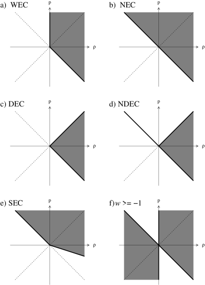
Figure 1: Shaded regions in the $\rho$-$p$ plane are those which obey the designated energy conditions. Illustrated are the Weak Energy Condition (WEC), Null Energy Condition (NEC), Dominant Energy Condition (DEC), Null Dominant Energy Condition (NDEC), the Strong Energy Condition (SEC), and the condition $w\geq-1$. Definitions of each condition are found in the text.

The most common energy conditions are the following:

• The Weak Energy Condition or WEC states that $T_{\mu\nu}t^{\mu}t^{\nu}\geq 0$ for all timelike vectors $t^{\mu}$, or equivalently that $\rho\geq 0$ and $\rho+p\geq 0$.

• The Null Energy Condition or NEC states that $T_{\mu\nu}\ell^{\mu}\ell^{\nu}\geq 0$ for all null vectors $\ell^{\mu}$, or equivalently that $\rho+p\geq 0$.

• The Dominant Energy Condition or DEC includes the WEC ($T_{\mu\nu}t^{\mu}t^{\nu}\geq 0$ for all timelike vectors $t^{\mu}$), as well as the additional requirement that $T^{\mu\nu}t_{\mu}$ is a non-spacelike vector (i.e., that $T_{\mu\nu}T^{\nu}{}_{\lambda}t^{\mu}t^{\lambda}\leq 0$). For a perfect fluid, these conditions together are equivalent to the simple requirement that $\rho\geq|p|$.

• The Null Dominant Energy Condition or NDEC is the DEC for null vectors only: for any null vector $\ell^{\mu}$, $T_{\mu\nu}\ell^{\mu}\ell^{\nu}\geq 0$ and $T^{\mu\nu}\ell_{\mu}$ is a non-spacelike vector. The allowed density and pressure are the same as for the DEC, except that negative densities are allowed so long as $p=-\rho$.

• The Strong Energy Condition or SEC states that $T_{\mu\nu}t^{\mu}t^{\nu}\geq{1\over 2}T^{\lambda}{}_{\lambda}t^{\sigma}t_{\sigma}$ for all timelike vectors $t^{\mu}$, or equivalently that $\rho+p\geq 0$ and $\rho+3p\geq 0$.

In Figure 1 we have plotted these conditions as restrictions on allowed regions of the $\rho$-$p$ plane. We have also plotted the condition $w\geq-1$ for comparison. Note that $w\geq-1$ is not equivalent to any of the energy conditions, although it is implied by the WEC, the DEC, and the NDEC.

The different energy conditions are used in different contexts — for example, the WEC and SEC are used in singularity theorems — and we will not review them in detail here (see hawkingellis for a discussion). Our present concern is to understand under what conditions a hypothetical dark energy component would be guaranteed to be stable. For this purpose, the relevant result is the “conservation theorem” of Hawking and Ellis hawkingellis ; Carter:2002wz . The conservation theorem invokes the DEC, and uses it to show that energy cannot propagate outside the light cone; in particular, if $T_{\mu\nu}$ vanishes on some closed region of a spacelike hypersurface, it will vanish everywhere in the future Cauchy development of that region — energy-momentum cannot spontaneously appear from nothing. A source obeying the DEC is therefore guaranteed to be stable.

For cosmological purposes, however, the DEC is somewhat too restrictive, as it excludes a negative cosmological constant (which is physically perfectly reasonable, even if it is not indicated by the data). This is why Garnavich:1998th advocated use of the NDEC in cosmology, since the NDEC is equivalent to the DEC except that negative values of $\rho$ are allowed so long as $p=-\rho$. Of course, the less restrictive NDEC invalidates the conservation theorem, as a simple example shows. Consider a theory with a negative vacuum energy $\rho_{\rm vac}<0$, and an ordinary scalar field $\psi$ (not a phantom) with potential $V(\psi)={1\over 2}m^{2}\psi^{2}$. Then both the vacuum energy and the scalar field obey the NDEC (although their sum may not, since the NDEC is a nonlinear constraint.) Imagine a field configuration with $\psi=\sqrt{-2\rho_{\rm vac}/m^{2}}$ and $\dot{\psi}=0$ everywhere throughout space. The energy-momentum tensor of this configuration is exactly zero [since $V(\psi)=-\rho_{\rm vac}$], but it would instantly begin evolving as $\psi$ rolled toward the minimum of its potential. There is nothing unphysical about such a situation, however, since a stable state is achieved once the field reaches $\psi=0$. The NDEC, therefore, does not guarantee stability with the confidence that the DEC does. However, it seems legitimate to ask that dynamical fields obey the DEC, while the cosmological constant is allowed as an exception.

The DEC implies that $w\geq-1$. (Indeed, for cosmological purposes we are interested in a source with $\rho>0$; in that case, all of the energy conditions imply $w\geq-1$.) Therefore, if we allow for pressures which are less than $-\rho$, we cannot guarantee the stability of the vacuum. The converse, however, is not true; a phantom component will not necessarily allow vacuum decay. In fact, since $p=w\rho$ is just a convenient parameterization and not strictly-speaking an equation of state, the issue of stability is somewhat complicated, as we shall see in the next few sections. Nevertheless, it seems very likely that energy sources which violate the DEC generally will be unstable, and this is what we will find in the specific example considered in Section V. Our philosophy, therefore, is neither to dismiss the possibility of DEC violation on the grounds that we cannot prove stability, nor to blithely accept DEC violation on the grounds that we cannot prove instability, but instead to see whether it is plausible that the timescale for instability could be sufficiently long so as to be irrelevant for practical purposes.

III Cosmological Evolution and Perturbations

Consider a flat Robertson-Walker universe with metric

$$ds^{2}=-dt^{2}+a^{2}(t)[dx^{2}+dy^{2}+dz^{2}]\ ,$$ (10)

for which the Einstein equations are the Friedmann equations (5) and (6). The cosmology and fate of a universe containing an energy component with constant $w<-1$ are relatively simple and have been examined in, for example, Caldwell:1999ew . As an example, consider the case in which the universe contains only dust and phantom matter. Then, if the universe ceases to be matter-dominated at cosmological time $t_{m}$, then the solution for the scale factor is

$$a(t)=a(t_{m})\left[-w+(1+w)\left(\frac{t}{t_{m}}\right)\right]^{2/3(1+w)}\ .$$ (11)

From this expression it is easy to see that phantom matter eventually comes to dominate the universe and that, since the Ricci scalar is given by

$$R=\frac{4(1-3w)}{3(1+w)^{2}}\left[t-\left(\frac{w}{1+w}\right)t_{m}\right]^{-2}\ ,$$ (12)

there is a future curvature singularity at $t=wt_{m}/(1+w)$. This occurs because, even though the energy densities in ordinary types of matter are redshifting away, the energy density in phantom matter increases in an expanding universe. Thus, the fate of the universe in these models Starobinsky:1999yw may be very different from that expected Starkman:1999pg ; Krauss:1999hj ; Avelino:2000ix ; Gudmundsson:2001gd ; Huterer:2002wf in $w>-1$ dark energy models.

It is, however, simple to construct models of phantom energy in which a future singularity is avoided. As we shall see in this section, scalar field models can yield a period of time in which the expansion proceeds with $w<-1$ and yet settles back to $w\geq-1$ (in our case $w=-1$) at even later times, thus sidestepping the predictions of $w=$ constant models. Consider a scalar field theory with action $S=\int{\cal L}\sqrt{|g|}\,d^{4}x$, and Lagrange density given by

$${\cal L}={1\over 2}g^{\mu\nu}(\partial_{\mu}\phi)(\partial_{\nu}\phi)-V(\phi)\ .$$ (13)

The notable feature of this model is that the sign of the kinetic term is reversed from its conventional value [in our conventions the usual expression would be $-{1\over 2}(\partial\phi)^{2}$]. The equation of motion for $\phi$ becomes

$$\ddot{\phi}+3H\dot{\phi}-a^{-2}\nabla^{2}\phi-V^{\prime}(\phi)=0\ ,$$ (14)

where $\nabla^{2}$ is the spatial Laplacian, $\nabla^{2}\phi=\partial_{x}^{2}\phi+\partial_{y}^{2}\phi+\partial_{x}^{2}\phi$, and a prime denotes differentiation with respect to $\phi$. Here the energy density $\rho_{\phi}$ and the pressure $p_{\phi}$ for a homogeneous $\phi$ field are given by

$$\rho_{\phi}=-{1\over 2}\dot{\phi}^{2}+V(\phi)\ ,$$ (15)

$$p_{\phi}=-{1\over 2}\dot{\phi}^{2}-V(\phi)\ ,$$ (16)

so that the equation-of-state parameter

$$w={p\over\rho}=\frac{{1\over 2}\dot{\phi}^{2}+V(\phi)}{{1\over 2}\dot{\phi}^{2}-V(\phi)}$$ (17)

satisfies $w\leq-1$.

We are interested in the cosmological evolution of this model and in the behavior of linearized perturbations of the phantom scalar field in the resulting cosmological background. As noted in Caldwell:1999ew , the spectrum of fluctuations of a phantom field evolves similarly to that for a quintessence field. Consider metric perturbations in the synchronous gauge,

$$ds^{2}=-dt^{2}+a^{2}(\delta_{ij}+h_{ij})dx^{i}dx^{j}\ .$$ (18)

A Fourier mode of the phantom field

$$\phi(t,{\bf k})={1\over\sqrt{2\pi}}\int\phi(t,{\bf x})e^{-i{\bf k}\cdot{\bf x}}\,d^{3}x$$ (19)

satisfies the equation of motion

$$\ddot{\delta\phi_{k}}+3H\dot{\delta\phi_{k}}+(k^{2}-V^{\prime\prime}){\delta\phi_{k}}=-\frac{1}{2}\dot{h}{\dot{\phi}},$$ (20)

where $h$ is the trace of the synchronous gauge metric perturbation $h_{ij}$. The effective mass for the perturbation is $(k^{2}-V^{\prime\prime})^{1/2}$. On large scales one may worry that this effective mass could become imaginary for a positive $V^{\prime\prime}$. We note, however, that a similar problem exists for a canonical scalar field for negative $V^{\prime\prime}$, and is thus easily avoided by the choice of potential; in particular, we may choose a potential with $V^{\prime\prime}<0$. An analysis of perturbations in more general non-canonical scalar field models is given in Garriga:1999 . In this paper, we will examine by explicit calculation the evolution of fluctuations in a specific model.

Figure 2: The gaussian potential energy of (21). The phantom scalar will evolve to the top of the hill and oscillate around the maximum.

Since scalar fields with negative kinetic terms evolve to the maxima of their classical potential, we consider a gaussian potential,

$$V(\phi)=V_{0}e^{-(\phi^{2}/\sigma^{2})}\ ,$$ (21)

where $V_{0}$ is the overall scale and $\sigma$ is a constant describing the width of the gaussian. The potential is represented in Figure 2. We obtained the cosmological evolution by numerically solving the equations of motion (5), (6), and (14). The initial conditions were $\phi_{\rm initial}=M_{\rm P}$ and $\dot{\phi}_{\rm initial}=0$, where $M_{\rm P}=(8\pi G)^{-1/2}$ is the reduced Planck mass. Since we require dark energy domination at the present epoch in the universe, with $\Omega_{X}\sim 0.7$ we choose $\sigma=M_{\rm P}$, $V_{0}=3M_{\rm P}^{2}H_{0}^{2}$. The results are plotted in figures 3,4 and 5.

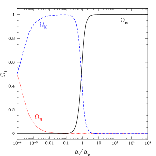
Figure 3: Evolution of the density parameters in radiation ($\Omega_{\rm R}$), matter ($\Omega_{\rm M}$), and the phantom field ($\Omega_{\phi}$).

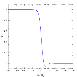
Figure 4: Evolution of the phantom field $\phi$ as a function of the scale factor.

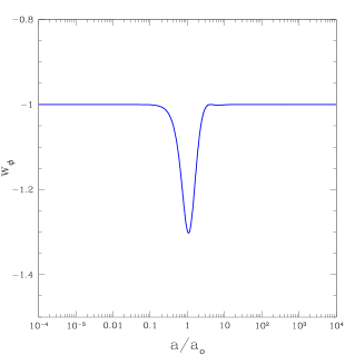
Figure 5: Evolution of the equation of state parameter $w$ for the phantom field as a function of the scale factor.

Note that during the initial stages of evolution the field $\phi$ is frozen by the expansion and acts as a negligibly small vacuum energy component (with $w\simeq-1$). However, at later times the field begins to evolve more rapidly towards the maximum of its potential, the energy density in the phantom field becomes cosmologically dominant, and during this period the equation of state parameter is much more negative. Finally, in the very late universe, the field comes to rest at the maximum of the potential and a period of $w=-1$ acceleration begins. Since $w$ is no longer less than $-1$, this ensures that there is no future singularity; rather, the universe eventually settles into a de Sitter phase.

Using the formalism for calculating fluctuations in a general matter field developed in Hu:1998 , one may calculate the effects of the fluctuations in this phantom field on the cosmic microwave background radiation (CMB). The resulting power spectrum of CMB fluctuations is shown in figure 6.

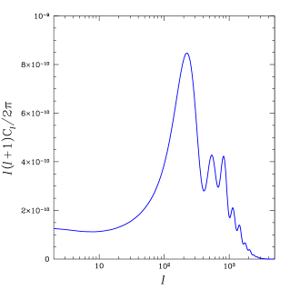
Figure 6: Predicted multipole moments $C_{l}$ for cosmic microwave background anisotropies.

We have not attempted a detailed parameter-fitting to CMB data, but it should be clear that our phantom model with the potential (21) does not predict any significant departures from conventional dark-energy scenarios; in particular, there is no evidence of dramatic instabilities distorting the power spectrum. (A more detailed study of the effect on the CMB power spectrum of phantom fields with a constant $w$ can be found in Schulz:2001yx .) However, the formalism for this analysis was based on linear perturbation theory, and it is quite plausible that instabilities only become manifest at higher orders. In the following sections we address this issue, first through numerical investigation of a model with two oscillators, and next by calculating the decay rate of phantom particles into phantoms plus gravitons.

IV Couplings to Normal Matter and Instability

Excitations of the scalar field from the model in the previous section have negative energy. The existence of negative energy particles may cause the system to be unstable due to interactions involving these particles.

In the next section we examine this possibility by estimating the tree level decay rate of negative energy phantom particles into other phantoms and gravitons. Before delving into that calculation, we will first try to build some intuition about possible instabilities by considering the classical evolution of a simple system, a coupled pair of simple harmonic oscillators. Conservation of energy limits the phase space of a coupled pair of oscillators when both oscillators have positive energy. Though the oscillators may exchange energy, neither oscillator may ever reach an energy greater than the total initial energy of the system. Allowing one of the oscillators to have negative energy removes this limitation on the phase space. In this case the positive energy oscillator may increase its energy to any level so long as the negative energy oscillator decreases its energy by a compensating amount. Hence the positive energy oscillator may reach arbitrarily high energies, and the negative energy oscillator may reach correspondingly large negative energies.

While conservation of energy does not prevent the oscillators in this simple model from reaching arbitrarily large energies, there is no guarantee that the system will be unstable in all regimes. In fact, the following analysis will show that for a weak coupling, the evolution of the energy of each oscillator exhibits a stable oscillation for an arbitrarily long time.

We consider a coupled pair of oscillators, one $\psi$ with positive energy, representing normal matter, and the other $\phi$ with negative energy, representing the phantom component.

$${\mathcal{L}}=\left({1\over 2}\dot{\psi}^{2}-m_{\psi}^{2}\psi^{2}\right)-\left({1\over 2}\dot{\phi}^{2}-m_{\phi}^{2}\phi^{2}\right)-\lambda\phi^{2}\psi^{2}\ ,$$ (22)

where $\lambda$ is a dimensionless coupling constant. We are interested in the evolution of the energy of each oscillator,

$$\rho_{\psi} = {1\over 2}\dot{\psi}^{2}+m_{\psi}^{2}$$

$$\rho_{\phi} = -\left({1\over 2}\dot{\phi}^{2}+m_{\phi}^{2}\right)\ .$$ (23)

The equations of motion are

$$\bar{\psi}^{\prime\prime} = -\left[\left(\frac{m_{\psi}}{m_{\phi}}\right)^{2}+\bar{\lambda}\bar{\phi}^{2}\right]\bar{\psi}$$

$$\bar{\phi}^{\prime\prime} = -\left[1-\bar{\lambda}\bar{\psi}^{2}\right]\bar{\phi}\ ,$$ (24)

where we have defined dimensionless rescaled variables

$$\bar{\phi} = \phi/M$$ (25)

$$\bar{\psi} = \psi/M$$ (26)

$$\bar{\lambda} = \lambda(M/m_{\phi})^{2}$$ (27)

$$\tau = m_{\phi}t\ .$$ (28)

In this section a prime denotes diferentiation with respect to the dimensionless time parameter $\tau$, and $M$ is the scale of the initial displacements of the oscillators.

We explore the stability of this model by integrating the equations of motion (IV) numerically for a range of parameters and initial conditions. Of particular interest are the simulations with $m_{\psi}=0$, in which one may think of the $\psi$ oscillator as analogous to the massless graviton. Three such simulations are shown in Fig. 7. In each of these integrations the oscillators are started at rest, displaced a distance $M$ from the origin. These plots are similar to those obtained for other initial conditions, and allowing the $\psi$ field to have a mass does not qualitatively change the plots shown here. Note that for $\bar{\lambda}<1$, $\rho_{\psi}$ and $\rho_{\phi}$ exhibit a stable oscillatory behavior, while for $\bar{\lambda}>1$, $\rho_{\psi}$ and $-\rho_{\phi}$ rapidly grow. From this analysis we conclude that this simple model is stable for small enough coupling but exhibits an instability for a large coupling. While the analysis of this simple model does not prove that a phantom field in the cosmological context will be stable to excitations and interactions with the gravitational field, it does provide some evidence that stability is possible.

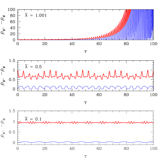
Figure 7: Evolution of the energies of a coupled pair of oscillators, one with positive energy, $\rho_{\psi}$ (thin line), and one with negative energy, $\rho_{\phi}$ (thick line), as a function of the rescaled coupling $\bar{\lambda}$. The oscillators are both started at rest displaced a distance $M$ from the origin, and the energies are expressed in units of $(m_{\phi}M)^{2}$. Note that for $\bar{\lambda}<1$, $\rho_{\psi}$ and $-\rho_{\phi}$ exhibit a stable oscillatory behavior, while for $\bar{\lambda}>1$, $\rho_{\psi}$ and $-\rho_{\phi}$ rapidly grow.

To make some connection to the cosmological model of the previous section, we consider how small the coupling in this simple model should be in order to have a stable solution. If we imagine a period of early universe inflation, then one expects perturbations in the phantom and gravitational fields to be of order $M\sim 10^{-5}M_{\rm P}$. The mass squared of the phantom field is

$$m_{\phi}^{2}=\frac{d^{2}V}{d\phi^{2}}\sim\frac{V_{0}}{M_{\rm P}^{2}}\sim(10^{-33}{\rm eV})^{2}\ .$$ (29)

The restriction $\bar{\lambda}<1$ then implies that the coupling in the Lagrangian satisfies $\lambda<10^{-110}$. While this at first seems to be an absurdly small number, we will see in the next section that, given the cosmological constraints of the previous section, such a coupling naturally results from considering perturbations of the phantom and gravitational fields.

V Phantom Decay Rate in Field Theory

The toy model of the previous section demonstrated that coupling a phantom oscillator to an ordinary oscillator results in a system which may or may not be unstable, depending on the magnitude of the coupling between them. It is far from clear, however, that this conclusion extends immediately to field theory. Roughly speaking, oscillators with some frequency correspond to field-theory modes of fixed wavelength; even if the model is stable when only certain wavelengths are considered, it does not follow that stability continues to obtain when integrating over all momenta.

One way of stating this concern is to ask about the decay rate of single particles that would conventionally be stable. Because excitations of the phantom field have negative energy, we could imagine a single particle decaying into a large number of phantoms and ordinary particles. The rate for this process can be calculated (at tree level) using ordinary Feynman diagrams. We will find that the rate is infinite when arbitrarily high momenta are included, but can be rendered finite if a cutoff (which might arise, for example, from higher-derivative terms in the action) is introduced.

Since we are interested in the allowed decay modes of phantom particles $\phi$ and their associated decay rates, it is instructive to first analyze the kinematics of reactions involving phantom fields. Let us adopt the convention that ordinary particles have 4-momenta with positive timelike component. Then, since our field has a negative kinetic term, the corresponding 4-momentum will have a negative timelike component. This leads to the following useful dictionary for translating between kinematically allowed reactions for phantom particles and those for ordinary particles.

Denote ordinary particles as $\psi$. To ask whether a certain reaction is kinematically allowed, we can just switch the phantom particles from the right side to the left and vice-versa, and ask whether the resulting reaction would normally be allowed. Consider for example the decay of an ordinary particle into another particle plus a phantom:

$$\psi_{1}\longrightarrow\psi_{2}+\phi\ .$$ (30)

This will be allowed if the reaction

$$\psi_{1}+\phi\longrightarrow\psi_{2}$$ (31)

would be allowed by conventional kinematics — in particular, if the mass of ordinary particle 2 were greater than the sum of the masses of ordinary particle 1 and the phantom. So it is clear that ordinary particles can decay into heavier particles plus phantoms. For example, if the electron were coupled to the phantom field, processes such as

$$e^{-}\rightarrow\mu^{-}+\nu_{e}+\bar{\nu}_{\mu}+\phi$$ (32)

would be allowed. The muon would then decay back into an electron, as part of a potentially disasterous cascade.

Next we turn to the decay of phantoms. First consider decays into ordinary particles

$$\phi\longrightarrow\psi_{1}+\psi_{2}$$ (33)

will be allowed if

$$\left|0\right\rangle\longrightarrow\phi+\psi_{1}+\psi_{2}$$ (34)

would be conventionally allowed, which it is not. However, consider a decay into one phantom and one ordinary particle:

$$\phi_{1}\longrightarrow\phi_{2}+\psi$$ (35)

will be allowed if

$$\phi_{2}\longrightarrow\phi_{1}+\psi$$ (36)

would ordinarily be, which requires $m_{\phi_{2}}>m_{\phi_{1}}+m_{\psi}$. So a phantom can decay into a heavier phantom plus a not-too-heavy ordinary particle.

If there is only one kind of phantom, one might think it would be stable since there would be no heavier phantoms to decay into. However, several lighter particles can mimic the 4-momentum of a heavier particle. Consider the decay of one phantom into two phantoms plus an ordinary particle:

$$\phi_{1}\longrightarrow\phi_{2}+\phi_{3}+\psi\ .$$ (37)

This will be allowed if

$$\phi_{2}+\phi_{3}\longrightarrow\phi_{1}+\psi$$ (38)

would ordinarily be, which it aways is for large enough relative velocities of $\phi_{2}$ and $\phi_{3}$.

In summary, if there is only one kind of phantom particle (with a unique mass), it can only decay by emitting at least two more phantoms, plus at least one ordinary particle. Ordinary particles, meanwhile, may decay into phantoms plus other ordinary particles with a larger effective mass than the original. A special case to these rules comes from massless particles. Although it would seem kinematically possible for massless particles to decay into massive particles plus phantoms, massless particles cannot decay in flat space (a reasonable approximation in the backgrounds we are considering) simply because there is no rest frame in which to calculate the rate — no proper time elapses along a null path.

Like any other dark-energy scalar field, the phantom should be weakly coupled to ordinary matter (or it would have been detected through fifth-force experiments or variation of the constants of nature Carroll:1998zi ). We therefore restrict our attention to only gravitons and phantoms. With the above rules in mind, the phantom decay channel involving the smallest number of particles is

$$\phi_{i}\rightarrow h+\phi_{1}+\phi_{2}\ ,$$ (39)

where $h$ is a graviton and $\phi$ is a phantom particle, illustrated in figure 8.

Figure 8: Decay of a phantom particle into two other phantoms and a graviton

Consider the specific model investigated in section III, a phantom scalar with potential

$$V(\phi)=V_{0}e^{-\phi^{2}/M_{\rm P}^{2}}\ .$$ (40)

We will first consider this potential expanded as a power series around some background value $\phi_{0}\sim M_{\rm P}$. Gravitons, meanwhile, may be represented by transverse-traceless metric perturbations $g_{\mu\nu}=g_{\mu\nu}^{(0)}+h_{\mu\nu}$, where $g_{\mu\nu}^{(0)}$ is the background Robertson-Walker metric. Strictly speaking, there is no way for a single graviton to couple non-derivatively to the potential, simply because there is no way to construct a scalar from a single traceless $h_{\mu\nu}$. But to avoid a surfeit of indices, and because it won’t affect the final answer, we will simply think of the graviton as a dimensionless scalar field $h$; to get a canonically-normalized field we multiply by $M_{\rm P}$.

To study the decay (39), we require the interaction part of the Lagrangian to first order in $h$ and third order in $\phi$, which is

$${\mathcal{L}}_{I} = \frac{1}{M_{\rm P}}(M_{\rm P}h)\frac{1}{3!}V^{\prime\prime\prime}(\phi_{0})\phi^{3}$$ (41)

$$= \lambda_{\rm eff}(M_{\rm P}h)\phi^{3}\ ,$$ (43)

where

$$\lambda_{\rm eff}\equiv 2\phi_{0}{V(\phi_{0})\over M_{\rm P}^{5}}\sim{V_{0}\over M_{\rm P}^{4}}\sim 10^{-120}\ .$$ (44)

The decay rate of a phantom particle through this channel is

$$\Gamma=\frac{1}{m_{\phi}}\int\frac{d^{3}p_{h}}{(2\pi)^{3}2E_{h}}\frac{d^{3}p_{\phi_{1}}}{(2\pi)^{3}2E_{\phi_{1}}}\frac{d^{3}p_{\phi_{2}}}{(2\pi)^{3}2E_{\phi_{2}}}|{\mathcal{M}}|^{2}(2\pi)^{4}\delta^{(4)}(p_{\phi_{i}}-p_{\phi_{1}}-p_{\phi_{2}}-p_{h})\ ,$$ (45)

where the matrix element $|{\mathcal{M}}|$ is just $\lambda_{\rm eff}$ at tree level. To get an upper limit on the reaction rate, and hence a lower limit on the timescale, we assume approximate isotropy, so $d^{3}p\sim|p|^{2}dp$. Because the relevant momenta are very large (and the masses very small), we can also approximate $E\sim p$. Putting all of this together we obtain

$$\Gamma\sim\frac{\lambda_{\rm eff}^{2}}{m_{\phi}}\int|p_{h}|dp_{h}\int|p_{\phi_{1}}|dp_{\phi_{1}}\int|p_{\phi_{2}}|dp_{\phi_{2}}\delta^{(4)}(p_{\phi_{i}}-p_{\phi_{1}}-p_{\phi_{2}}-p_{h})\ .$$ (46)

If we take the limits on the integrals to be $\infty$, the decay rate is clearly infinite. Hence, the answer to our investigation into instability seems very clear: the theory is dramatically unstable, as individual particles rapidly decay into cascades of phantoms and gravitons.

However, our philosophy has been to think of this model as an effective theory valid at low energies. The reason why the decay rate diverges is because the phase space is infinite, since the phantoms can have arbitrarily large negative energies. Therefore, this result relies on taking the calculation at face value up to infinite momentum transfer. Instead, we should only trust the phase-space integrals up to some cutoff where new physics might enter. For example, we could imagine a higher-derivative term of the form

$${\mathcal{L}}\sim-(\partial\phi)^{4}\ ,$$ (47)

which would eventually dominate over the negative-kinetic-energy term we have already introduced.

We have not investigated closely the properties of phantom models with higher-derivative terms. Instead, let us crudely approximate the effect of a momentum cutoff at a scale $\Lambda$ by only allowing the phase-space integrals to range up to that cutoff. Looking at (46), we can estimate the truncated decay rate as

$$\Gamma\sim\lambda_{\rm eff}^{2}\frac{\Lambda^{2}}{m_{\phi}}\ .$$ (48)

The timescale for decay is $\tau=\Gamma^{-1}$. Despite any fundamental instability, a model will be phenomenologically viable if the lifetime is greater than the Hubble time $H_{0}^{-1}\sim 10^{60}M_{\rm P}^{-1}$. Recalling that $m_{\phi}\sim 10^{-60}M_{\rm P}$ and $\lambda_{\rm eff}\sim 10^{-120}$, the lifetime in units of the Hubble time is

$$H_{0}\tau\sim 10^{120}\left(\frac{M_{\rm P}}{\Lambda}\right)^{2}\ .$$ (49)

In other words, the lifetime from this decay channel exceeds cosmological timescales so long as $\Lambda<10^{60}M_{\rm P}$, which is certainly not a stringent constraint.

However, the infinite phase space for this one decay is not the only infinity we have to deal with; a single phantom can decay into arbitrary numbers of gravitons and phantoms, so we must sum over all the channels. For each new final-state particle $\Gamma$ gets multiplied by a factor of $(\Lambda/M_{\rm P})^{2}$. The $\Lambda^{2}$ comes from the new momentum integral, and the $M_{\rm P}^{-2}$ is introduced into $\lambda_{\rm eff}^{2}$. So, if we denote the decay rate (48) by $\Gamma_{0}$, then if there are $n$ additional particles in the final state the total decay rate is given by

$$\Gamma_{n}=\left(\frac{\Lambda}{M_{\rm P}}\right)^{2n}\Gamma_{0}\ ,$$ (50)

Therefore, the total decay rate is

$$\Gamma_{\rm total}=\sum_{n=0}^{\infty}(n+1)\Gamma_{n}\ ,$$ (51)

where the factor $(n+1)$ comes from the number of different ways the final state can be composed of gravitons and phantoms. This yields

$$\Gamma_{\rm total}=\Gamma_{0}\left[1-\left(\frac{\Lambda}{M_{\rm P}}\right)^{2}\right]^{-2}\ .$$ (52)

Thus, the decay rate remains of order $\Gamma_{0}$ so long as $\Lambda$ is not larger than $M_{\rm P}$. This still seems like a comfortable result.

There is, however, one more possibility to be accounted for. Part of the reason we obtained reasonable decay rates from interactions originating in the potential $V(\phi)$ was because of the small value of $V_{0}\sim(10^{-3}{\rm~{}eV})^{4}$. This suppression is lost if we consider couplings of gravitons to derivatives of $\phi$. Since we are claiming that our model is simply an effective field theory, we are obligated to include all possible non-renormalizable interactions, suppressed by appropriate powers of the cutoff scale. Consider for example the operator

$${\mathcal{L}}={\beta\over M_{\rm P}\Lambda}\phi(M_{\rm P}h^{\mu\nu})\partial_{\mu}\phi\partial_{\nu}\phi\ ,$$ (53)

where $\beta$ is a dimensionless coupling. (We will use the same cutoff $\Lambda$ for our non-renormalizable terms as in our momentum integrals; the $M_{\rm P}$ in the denominator comes from normalization of $h^{\mu\nu}$.) This term will also contribute to the interaction shown in Figure 8. Following similar logic as above (including two powers of the momentum in ${\mathcal{M}}$ from the derivatives), we get

$$\Gamma\sim{\beta^{2}\Lambda^{4}\over m_{\phi}M_{\rm P}^{2}}\ .$$ (54)

Using $H_{0}\sim m_{\phi}\sim 10^{-60}M_{\rm P}$, the lifetime in units of the Hubble time is now

$$H_{0}\tau\sim\beta^{-2}\left({M_{\rm P}\over 10^{30}\Lambda}\right)^{4}\ .$$ (55)

Therefore, if $\beta$ is of order unity, to obtain cosmologically viable decay rates ($H_{0}\tau>1$) we require the cutoff to be

$$\Lambda<10^{-30}M_{\rm P}\sim 10^{-3}{\rm eV}\ .$$ (56)

This is a much smaller cutoff than was required when we considered coupling through the potential, since the small prefactor $V_{0}$ is not around to help us.

The above result is alleviated somewhat by imposing an approximate global symmetry on the theory, that the Lagrangian density be invariant under $\phi\rightarrow\phi+{\rm constant}$. Such a symmetry is quite reasonable, as it is the only known way to ensure both a nearly-flat potential and appropriately small couplings to ordinary matter Carroll:1998zi . In this case, the irrelevant operator of lowest dimension leading to phantom decay into gravitons is

$${\cal L}=\frac{\gamma}{M_{\rm P}^{2}\Lambda^{4}}\left[(M_{\rm P}h^{\mu\nu})\partial_{\mu}\phi\partial_{\nu}\phi\right]^{2}\ .$$ (57)

The decay rate is then

$$\Gamma\sim{\gamma^{2}\Lambda^{6}\over m_{\phi}M_{\rm P}^{4}}\ ,$$ (58)

with an associated lifetime

$$H_{0}\tau\sim\gamma^{-2}\left({M_{\rm P}\over 10^{20}\Lambda}\right)^{6}\ ,$$ (59)

which, if $\gamma\sim 1$, leads to the relaxed requirement $\Lambda<10^{-20}M_{\rm P}\sim 100$ MeV.

Under our most optimistic assumptions (of an approximate global symmetry), we therefore find that the momentum cutoff characterizing our effective theory must be less than 100 MeV to guarantee that the instability timescale is greater than the age of the universe. We find this value to be uncomfortably low, although not necessarily impossible; dark-energy models are typically characterized by energy scales $\sim 10^{-3}$ eV (for the vacuum energy today) and $\sim 10^{-33}$ eV (for the mass of the scalar field), so perhaps the scalar field theory is only valid up to relatively low momenta. Alternatively, one might imagine searching for some mechanism which would suppress derivative couplings, leaving only the couplings of gravitons to the potential, which were consistent with a cutoff as high as the Planck scale.

VI Conclusions

There is no doubt that the discovery of a new component of the energy density of the universe has profound implications for the relationship between particle physics and gravity. Whether this component be a pure cosmological constant (whose magnitude we have no idea how to understand), a dynamical component Sahni:1999gb ; Parker:1999td ; Chiba:1999ka ; Boisseau:2000pr ; Schulz:2001yx ; Faraoni:2001tq ; maor2 ; Onemli:2002hr ; Torres:2002pe ; Frampton:2002tu ; Wetterich:fm ; Ratra:1987rm ; Caldwell:1997ii ; Armendariz-Picon:1999rj ; Armendariz-Picon:2000dh ; Armendariz-Picon:2000ah ; Mersini:2001su (whose special interactions give rise to the tiny vacuum energy we observe) or an as yet unimagined source, its nature is an outstanding problem of fundamental physics. The data thus far, although pointing conclusively to the existence of this dark energy, do not allow us to distinguish between competing scenarios. In particular, much of the allowed parameter space lies in the region $w<-1$ in which some cherished notion behind our present theories must be sacrificed.

There are several ways in which one may achieve $w<-1$, including purely negative kinetic terms, non-minimal kinetic terms, and scalar-tensor theories. In addition, one might imagine that effective superexponential expansion of the universe might be obtained by modifying the Friedmann equation. While this is at odds with a purely four-dimensional general relativistic description of the universe, such an effect might be obtained in the context of brane-world models Kehagias:1999aa . However, any such modification of the Friedmann equation must avoid conflict with the precision predictions of primordial nucleosynthesis Tegmark:2001zc ; Carroll:2001bv ; Zahn:2002rr .

In this paper we have taken seriously the possibility that $w$ may be less than $-1$ and have asked the question: “From a particle-physics and general-relativistic point of view, can such theories be made consistent?” In particular, we have considered a specific toy model in which the null dominant energy condition is violated and hence the resulting space-time may be unstable. In this model the cosmology is well-behaved and the theory may be constructed so that it is stable to small, linear perturbations. When we consider higher order effects, however, the model fails to remain stable. The central result of this paper is a field theory calculation of the decay rate of phantom particles into gravitons. This decay rate would be infinite if the phantom theory was fundamental, valid up to arbitrarily high momenta, and would render the theory useless as a dark energy candidate. We therefore consider the phantom theory to be an effective theory valid below a scale $\Lambda$. Interestingly, couplings of gravitons to an appropriate scalar potential do not lead to decay of phantoms into gravitons and other phantoms on sub-Hubble timescales, so long as the cutoff $\Lambda$ is below the Planck scale. However, in such an effective field theory approach, we are mandated to include in the Lagrangian operators of all possible dimensions, suppressed by suitable powers of the cutoff scale. In particular, we must include couplings of gravitons to derivatives of the phantom field. We find that such operators, even though they may be of high order, can lead to unacceptably short lifetimes for phantom particles unless the cutoff scale is less than $100$ MeV, so new physics must appear in the phantom sector at scales lower than this.

Our analysis demonstrates that a model with a well-behaved cosmological evolution and stability to linear perturbations may still exhibit instability due to higher order interactions. We may therefore ask another crucial question: “Should observers seeking to constrain cosmological parameters take seriously the possibility that $w<-1$?” Unfortunately the answer is somewhat ambiguous. On the one hand, we know of no easy way to construct a viable model of this sort; on the other, it is certainly conceivable that new physics in the dark-energy sector kicks in at low scales to render a phantom model stable, or that phantom behavior is mimicked by even more exotic mechanisms (such as modifications of the Friedmann equation). Therefore, whether or not observations constrain $w$ to be greater than or equal to $-1$ is still an interesting question, although there is a substantial a priori bias against the possibility. For theorists, our conclusion is more straightforward: the onus is squarely on would-be phantom model-builders to show how any specific proposal manages to avoid rapid vacuum decay.

References

- (1) A. G. Riess et al. [Supernova Search Team Collaboration], Astron. J. 116, 1009 (1998) [arXiv:astro-ph/9805201].
- (2) S. Perlmutter et al. [Supernova Cosmology Project Collaboration], Astrophys. J. 517, 565 (1999) [arXiv:astro-ph/9812133].
- (3) S. M. Carroll, Living Rev. Rel. 4, 1 (2001) [arXiv:astro-ph/0004075].
- (4) P. J. Peebles and B. Ratra, arXiv:astro-ph/0207347.
- (5) P. M. Garnavich et al., Astrophys. J. 509, 74 (1998) [arXiv:astro-ph/9806396].
- (6) H. P. Nilles, Phys. Rept. 110, 1 (1984).
- (7) J. D. Barrow, Nucl. Phys. B 310, 743 (1988).
- (8) M. D. Pollock, Phys. Lett. B 215, 635 (1988).
- (9) R. R. Caldwell, arXiv:astro-ph/9908168.
- (10) V. Sahni and A. A. Starobinsky, Int. J. Mod. Phys. D 9, 373 (2000) [arXiv:astro-ph/9904398].
- (11) L. Parker and A. Raval, Phys. Rev. D 60, 063512 (1999) [arXiv:gr-qc/9905031].
- (12) T. Chiba, T. Okabe and M. Yamaguchi, Phys. Rev. D 62, 023511 (2000) [arXiv:astro-ph/9912463].
- (13) B. Boisseau, G. Esposito-Farese, D. Polarski and A. A. Starobinsky, Phys. Rev. Lett. 85, 2236 (2000) [arXiv:gr-qc/0001066].
- (14) A. E. Schulz and M. J. White, Phys. Rev. D 64, 043514 (2001) [arXiv:astro-ph/0104112].
- (15) V. Faraoni, Int. J. Mod. Phys. D 11, 471 (2002) [arXiv:astro-ph/0110067].
- (16) I. Maor, R. Brustein, J. McMahon and P. J. Steinhardt, Phys. Rev. D 65, 123003 (2002). [arXiv:astro-ph/0112526].
- (17) V. K. Onemli and R. P. Woodard, Class. Quant. Grav. 19, 4607 (2002) [arXiv:gr-qc/0204065].
- (18) D. F. Torres, Phys. Rev. D 66, 043522 (2002) [arXiv:astro-ph/0204504].
- (19) P. H. Frampton, arXiv:astro-ph/0209037.
- (20) S. Hannestad and E. Mortsell, Phys. Rev. D 66, 063508 (2002) [arXiv:astro-ph/0205096].
- (21) A. Melchiorri, L. Mersini, C. J. Odman and M. Trodden, arXiv:astro-ph/0211522.
- (22) B. McInnes, arXiv:astro-ph/0210321.
- (23) S.W. Hawking and G.F.R. Ellis, The Large Scale Structure of Space-Time, (Cambridge, Cambridge University Press: 1973).
- (24) B. Carter, arXiv:gr-qc/0205010.
- (25) J. Garriga and V. Mukhanov, Phys. Lett. B 458, 219 (1999) [arXiv:hep-th/9904176].
- (26) W. Hu, Astrophys. J. 506, 485 (1998) [arXiv:astro-ph/9801234].
- (27) A. A. Starobinsky, Grav. Cosmol. 6, 157 (2000) [arXiv:astro-ph/9912054].
- (28) G. Starkman, M. Trodden and T. Vachaspati, Phys. Rev. Lett. 83, 1510 (1999) [arXiv:astro-ph/9901405].
- (29) L. M. Krauss and G. D. Starkman, Astrophys. J. 531, 22 (2000) [arXiv:astro-ph/9902189].
- (30) P. P. Avelino, J. P. de Carvalho and C. J. Martins, Phys. Lett. B 501, 257 (2001) [arXiv:astro-ph/0002153].
- (31) E. H. Gudmundsson and G. Bjornsson, Astrophys. J. 565, 1 (2002) [arXiv:astro-ph/0105547].
- (32) D. Huterer, G. D. Starkman and M. Trodden, Phys. Rev. D 66, 043511 (2002) [arXiv:astro-ph/0202256].
- (33) S. M. Carroll, Phys. Rev. Lett. 81, 3067 (1998) [arXiv:astro-ph/9806099].
- (34) C. Barcelo and M. Visser, arXiv:gr-qc/0205066.
- (35) B. McInnes, arXiv:hep-th/0212014.
- (36) C. Armendariz-Picon, Phys. Rev. D 65, 104010 (2002) [arXiv:gr-qc/0201027].
- (37) C. Wetterich, Nucl. Phys. B 302, 668 (1988).
- (38) B. Ratra and P. J. Peebles, Phys. Rev. D 37, 3406 (1988).
- (39) R. R. Caldwell, R. Dave and P. J. Steinhardt, Phys. Rev. Lett. 80, 1582 (1998) [arXiv:astro-ph/9708069].
- (40) C. Armendariz-Picon, T. Damour and V. Mukhanov, Phys. Lett. B 458, 209 (1999) [arXiv:hep- th/9904075].
- (41) C. Armendariz-Picon, V. Mukhanov and P. J. Steinhardt, Phys. Rev. Lett. 85, 4438 (2000) [arXiv:astro-ph/0004134].
- (42) C. Armendariz-Picon, V. Mukhanov and P. J. Steinhardt, Phys. Rev. D 63, 103510 (2001) [arXiv:astro-ph/0006373].
- (43) L. Mersini, M. Bastero-Gil and P. Kanti, Phys. Rev. D 64, 043508 (2001) [arXiv:hep-ph/0101210].
- (44) A. Kehagias, arXiv:hep-th/9911134.
- (45) M. Tegmark, Phys. Rev. D 66, 103507 (2002) [arXiv:astro-ph/0101354].
- (46) S. M. Carroll and M. Kaplinghat, Phys. Rev. D 65, 063507 (2002) [arXiv:astro-ph/0108002].
- (47) O. Zahn and M. Zaldarriaga, arXiv:astro-ph/0212360.