Generation of large-scale vorticity in a homogeneous turbulence
with a mean velocity shear

Abstract

An effect of a mean velocity shear on a turbulence and on the effective force which is determined by the gradient of Reynolds stresses is studied. Generation of a mean vorticity in a homogeneous incompressible turbulent flow with an imposed mean velocity shear due to an excitation of a large-scale instability is found. The instability is caused by a combined effect of the large-scale shear motions (”skew-induced” deflection of equilibrium mean vorticity) and ”Reynolds stress-induced” generation of perturbations of mean vorticity. Spatial characteristics, such as the minimum size of the growing perturbations and the size of perturbations with the maximum growth rate, are determined. This instability and the dynamics of the mean vorticity are associated with the Prandtl’s turbulent secondary flows. This instability is similar to the mean-field magnetic dynamo instability. Astrophysical applications of the obtained results are discussed.

I Introduction

Vorticity generation in turbulent and laminar flows was studied experimentally, theoretically and numerically in a number of publications (see, e.g., P52 ; T56 ; B87 ; BB64 ; P70 ; M84 ; GHW02 ; PA02 ; C94 ; T98 ; RAO98 ; P87 ; GLM97 ). For instance, a mechanism of the vorticity production in laminar compressible fluid flows consists in the misalignment of pressure and density gradients P87 ; GLM97 . It was shown in GLM97 that the vorticity generation represents a generic property of any slow nonadiabatic laminar gas flow. In incompressible flows this effect does not occur. The role of small-scale vorticity production in incompressible turbulent flows was discussed in T98 .

On the other hand, generation and dynamics of the mean vorticity are associated with turbulent secondary flows (see, e.g., P52 ; B87 ; BB64 ; P70 ; M84 ; GHW02 ; PA02 ). These flows, e.g., arise at the lateral boundaries of three-dimensional thin shear layers whereby longitudinal (streamwise) mean vorticity is generated by a lateral deflection or ”skewing” of an existing shear layer B87 . The skew-induced streamwise mean vorticity generation corresponds to Prandtl’s first kind of secondary flows. In turbulent flows, e.g., in straight noncircular ducts, streamwise mean vorticity can be generated by the Reynolds stresses. The latter is Prandtl’s second kind of turbulent secondary flows, and it ”has no counterpart in laminar flow and cannot be described by any turbulence model with an isotropic eddy viscocity” B87 .

In the present study we demonstrated that in a homogeneous incompressible turbulent flow with an imposed mean velocity shear a large-scale instability can be excited which results in a mean vorticity production. This instability is caused by a combined effect of the large-scale shear motions (”skew-induced” deflection of equilibrium mean vorticity) and ”Reynolds stress-induced” generation of perturbations of mean vorticity. The ”skew-induced” deflection of equilibrium mean vorticity $\bar{\bf W}^{(s)}$ is determined by $(\bar{\bf W}^{(s)}\cdot\mbox{\boldmath$\nabla$})\tilde{\bf U}$-term in the equation for the mean vorticity, where $\tilde{\bf U}$ are perturbations of the mean velocity (see below). The ”Reynolds stress-induced” generation of a mean vorticity is determined by $\mbox{\boldmath$\nabla$}{\bf\times}\mbox{\boldmath$\cal F$},$ where $\cal F$ is an effective force caused by a gradient of Reynolds stresses.

This instability is similar to the mean-field magnetic dynamo instability (see, e.g., M78 ) which is caused by a combined effect of a nonuniform mean flow (differential rotation or large-scale shear motions) and turbulence effects (helical turbulent motions which produce the $\alpha$ effect M78 or anisotropic turbulent motions which cause the ”shear-current” effect RK03 ).

This paper is organized as follows. In Section II the governing equations are formulated. In Section III the general form of the Reynolds stresses in a homogeneous turbulence with an imposed mean velocity shear is found using simple symmetry reasoning, and the mechanism for the large-scale instability caused by a combined effect of the large-scale shear motions and ”Reynolds stress-induced” generation of perturbations of the mean vorticity is discussed. In Section IV the equation for the second moment of velocity fluctuations in a homogeneous turbulence with an imposed mean velocity shear is derived. This allows us to study an effect of a mean velocity shear on a turbulence and to calculate the effective force determined by the gradient of Reynolds stresses. Using the derived mean-field equation for vorticity we studied in Section IV the large-scale instability which causes the mean vorticity production.

II The governing equations

Our goal is to study an effect of mean velocity shear on a turbulence and on a dynamics of a mean vorticity. The equation for the evolution of vorticity ${\bf W}\equiv\mbox{\boldmath$\nabla$}{\bf\times}{\bf v}$ reads

$${\partial{\bf W}\over\partial t}=\mbox{\boldmath$\nabla$}{\bf\times}({\bf v}{\bf\times}{\bf W}-\nu\mbox{\boldmath$\nabla$}{\bf\times}{\bf W})\;,$$ (1)

where ${\bf v}$ is the fluid velocity with $\mbox{\boldmath$\nabla$}\cdot{\bf v}=0$ and $\nu$ is the kinematic viscosity. This equation follows from the Navier-Stokes equation. In this study we use a mean field approach whereby the velocity and vorticity are separated into the mean and fluctuating parts: ${\bf v}=\bar{\bf U}+{\bf u}$ and ${\bf W}=\bar{\bf W}+{\bf w},$ the fluctuating parts have zero mean values, and $\bar{\bf U}=\langle{\bf v}\rangle,$ $\,\bar{{\bf W}}=\langle{\bf W}\rangle.$ Averaging Eq. (1) over an ensemble of fluctuations we obtain an equation for the mean vorticity $\bar{{\bf W}}$

$${\partial\bar{{\bf W}}\over\partial t}=\mbox{\boldmath$\nabla$}{\bf\times}(\bar{\bf U}{\bf\times}\bar{{\bf W}}+\langle{\bf u}{\bf\times}{\bf w}\rangle-\nu\mbox{\boldmath$\nabla$}{\bf\times}\bar{{\bf W}})\;.$$ (2)

Note that the effect of turbulence on the mean vorticity is determined by the Reynolds stresses $\langle u_{i}u_{j}\rangle,$ because

$$\langle{\bf u}{\bf\times}{\bf w}\rangle_{i}=-\nabla_{j}\langle u_{i}u_{j}\rangle+{1\over 2}\nabla_{i}\langle{\bf u}^{2}\rangle\;,$$ (3)

and curl of the last term in Eq. (3) vanishes.

We consider a turbulent flow with an imposed mean velocity shear $\nabla_{i}\bar{\bf U}^{(s)},$ where $\bar{\bf U}^{(s)}$ is a steady state solution of the Navier-Stokes equation for the mean velocity field. In order to study a stability of this equilibrium we consider perturbations $\tilde{\bf U}$ of the mean velocity, i.e., the total mean velocity is $\bar{\bf U}=\bar{\bf U}^{(s)}+\tilde{\bf U}.$ Similarly, the total mean vorticity is $\bar{\bf W}=\bar{\bf W}^{(s)}+\tilde{\bf W},$ where $\bar{\bf W}^{(s)}=\mbox{\boldmath$\nabla$}{\bf\times}\bar{\bf U}^{(s)}$ and $\tilde{\bf W}=\mbox{\boldmath$\nabla$}{\bf\times}\tilde{\bf U}.$ Thus, the linearized equation for the small perturbations of the mean vorticity, $\tilde{{\bf W}}=\bar{{\bf W}}-\bar{\bf W}^{(s)},$ is given by

$${\partial\tilde{{\bf W}}\over\partial t}=\mbox{\boldmath$\nabla$}{\bf\times}(\bar{\bf U}^{(s)}{\bf\times}\tilde{{\bf W}}+\tilde{\bf U}{\bf\times}\bar{\bf W}^{(s)}+\mbox{\boldmath$\cal F$}-\nu\mbox{\boldmath$\nabla$}{\bf\times}\tilde{{\bf W}})\;,$$ (4)

where ${\cal F}_{i}=-\nabla_{j}[f_{ij}(\bar{\bf U})-f_{ij}(\bar{\bf U}^{(s)})]$ is the effective force and $f_{ij}=\langle u_{i}u_{j}\rangle.$ Equation (4) is derived by subtracting Eq. (2) written for $\bar{\bf W}^{(s)}$ from the corresponding equation for the mean vorticity $\bar{{\bf W}}.$ In order to obtain a closed system of equations in Section IV we derived an equation for the effective force $\mbox{\boldmath$\cal F$}.$ Equation (4) determines the dynamics of perturbations of the mean vorticity. In the next Sections we will show that under certain conditions the large-scale instability can be excited which causes the mean vorticity production.

III The qualitative description

In this Section we discuss the mechanism of the large-scale instability. The mean velocity shear can affect a turbulence. The reason is that additional strongly anisotropic velocity fluctuations can be generated by tangling of the mean-velocity gradients with the Kolmogorov-type turbulence (see FIG. 1). The source of energy of this ”tangling turbulence” is the energy of the Kolmogorov turbulence EKRZ02 . The tangling turbulence is an universal phenomenon, e.g., it was introduced by Wheelon W57 and Batchelor et al. BH59 for a passive scalar and by Golitsyn G60 and Moffatt M61 for a passive vector (magnetic field). Anisotropic fluctuations of a passive scalar (e.g., the number density of particles or temperature) are produced by tangling of gradients of the mean passive scalar field with a random velocity field. Similarly, anisotropic magnetic fluctuations are generated by tangling of the mean magnetic field with the velocity fluctuations. The Reynolds stresses in a turbulent flow with a mean velocity shear is another example of a tangling turbulence. Indeed, they are strongly anisotropic in the presence of shear and have a steeper spectrum $(\propto k^{-7/3})$ than a Kolmogorov turbulence (see, e.g., L67 ; WC72 ; SV94 ; IY02 ; EKRZ02 ). The anisotropic velocity fluctuations of tangling turbulence were studied first by Lumley L67 .

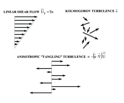
Figure 1: Mechanism for the tangling turbulence: generation of anisotropic velocity fluctuations by tangling of the mean velocity gradients with the Kolmogorov-type turbulence.

The general form of the Reynolds stresses in a turbulent flow with a mean velocity shear can be obtained from simple symmetry reasoning. Indeed, the Reynolds stresses $\langle u_{i}u_{j}\rangle$ is a symmetric true tensor. In a turbulent flow with an imposed mean velocity shear, the Reynolds stresses depend on the true tensor $\nabla_{j}\bar{U}_{i},$ which can be written as a sum of the symmetric and antisymmetric parts, i.e., $\nabla_{j}\bar{U}_{i}=(\partial\hat{U})_{ij}-(1/2)\varepsilon_{ijk}\,\bar{W}_{k},$ where $(\partial\hat{U})_{ij}=(\nabla_{i}\bar{U}_{j}+\nabla_{j}\bar{U}_{i})/2$ is the true tensor and $\bar{\bf W}=\mbox{\boldmath$\nabla$}{\bf\times}\bar{\bf U}$ is the mean vorticity (pseudo-vector). We take into account the effect which is linear in perturbations $(\partial\tilde{U})_{ij}$ and $\tilde{\bf W},$ where $(\partial\tilde{U})_{ij}=(\nabla_{i}\tilde{U}_{j}+\nabla_{j}\tilde{U}_{i})/2.$ Thus, the general form of the Reynolds stresses can be found using the following true tensors: $(\partial\tilde{U})_{ij},$ $\,M_{ij},$ $\,N_{ij},$ $\,H_{ij}$ and $G_{ij},$ where

$$M_{ij} = (\partial\bar{U}^{(s)})_{im}({\partial\tilde{U}})_{mj}+(\partial\bar{U}^{(s)})_{jm}({\partial\tilde{U}})_{mi}\;,$$ (5)

$$N_{ij} = \tilde{W}_{n}[\varepsilon_{nim}(\partial\bar{U}^{(s)})_{mj}+\varepsilon_{njm}(\partial\bar{U}^{(s)})_{mi}]\;,$$ (6)

$$H_{ij} = \bar{W}^{(s)}_{n}[\varepsilon_{nim}(\partial\tilde{U})_{mj}+\varepsilon_{njm}(\partial\tilde{U})_{mi}]\;,$$ (7)

$$G_{ij} = \bar{W}^{(s)}_{i}\tilde{W}_{j}+\bar{W}^{(s)}_{j}\tilde{W}_{i}\;,$$ (8)

$(\partial\bar{U}^{(s)})_{ij}=(\nabla_{i}\bar{U}^{(s)}_{j}+\nabla_{j}\bar{U}^{(s)}_{i})/2$ and $\varepsilon_{ijk}$ is the fully antisymmetric Levi-Civita tensor (pseudo-tensor). Therefore, the Reynolds stresses have the following general form:

$$f_{ij}(\tilde{\bf U}) = -2\nu_{{}_{T}}\,(\partial\tilde{U})_{ij}-l_{0}^{2}\,(B_{1}\,M_{ij}$$ (9)

$$+B_{2}\,N_{ij}+B_{3}\,H_{ij}+B_{4}\,G_{ij})\;,$$

where $B_{k}$ are the unknown coefficients, $l_{0}$ is the maximum scale of turbulent motions, $\nu_{{}_{T}}=l_{0}u_{0}/\beta$ is the turbulent viscosity with the factor $\,\beta\approx 3-6,$ and $u_{0}$ is the characteristic turbulent velocity in the maximum scale of turbulent motions $l_{0}.$ The parameter $l_{0}^{2}$ in Eq. (9) was introduced using dimensional arguments. The first term in RHS of Eq. (9) describes the standard isotropic turbulent viscosity, whereas other terms are determined by fluctuations caused by the imposed velocity shear $\nabla_{i}\bar{U}^{(s)}_{j}.$

Let us study the evolution of the mean vorticity using Eqs. (4) and (9), where ${\cal F}_{i}=-\nabla_{j}f_{ij}(\tilde{\bf U})$ is the effective force. We consider a homogeneous divergence-free turbulence with a mean velocity shear, e.g., $\bar{\bf U}^{(s)}=(0,Sx,0)$ and $\bar{\bf W}^{(s)}=(0,0,S).$ For simplicity we use perturbations of the mean vorticity in the form $\tilde{{\bf W}}=(\tilde{W}_{x}(z),\tilde{W}_{y}(z),0).$ Then Eq. (4) can be written as

$${\partial\tilde{W}_{x}\over\partial t} = S\tilde{W}_{y}+\nu_{{}_{T}}\tilde{W}^{\prime\prime}_{x}\;,$$ (10)

$${\partial\tilde{W}_{y}\over\partial t} = -\alpha\,S\,l_{0}^{2}\,\tilde{W}^{\prime\prime}_{x}+\nu_{{}_{T}}\tilde{W}^{\prime\prime}_{y}\;,$$ (11)

where $\tilde{W}^{\prime\prime}_{x}=\partial^{2}\tilde{W}_{x}/\partial z^{2},$ $\,\alpha=(B_{1}+2(B_{2}+B_{3})-4B_{4})/4.$ In Eq. (10) we took into account that $l_{0}^{2}\tilde{W}^{\prime\prime}_{y}\ll\tilde{W}_{y},$ i.e., the characteristic scale $L_{W}$ of the mean vorticity variations is much larger than the maximum scale of turbulent motions $l_{0}.$ This assumption corresponds to the mean-field approach. For derivation of Eqs. (10) and (11) we used the identities presented in Appendix A.

We seek for a solution of Eqs. (10) and (11) in the form $\propto\exp(\gamma t+iKz).$ Thus, when $\alpha>0$ perturbations of the mean vorticity can grow in time and the growth rate of the instability is given by

$$\gamma=\sqrt{\alpha}\,S\,l_{0}\,K-\nu_{{}_{T}}\,K^{2}\;.$$ (12)

The maximum growth rate of perturbations of the mean vorticity, $\gamma_{\rm max}=\alpha\,(S\,l_{0})^{2}/4\nu_{{}_{T}},$ is attained at $K=K_{m}=\sqrt{\alpha}\,S\,l_{0}/2\nu_{{}_{T}}.$ The sufficient condition $\gamma>0$ for the excitation of the instability reads $L_{W}/l_{0}>2\pi/(\beta\,\sqrt{\alpha}\,\tau_{0}S),$ where $L_{W}\equiv 2\pi/K$ and we consider a weak velocity shear $\tau_{0}S\ll 1.$

Now let us discuss the mechanism of this instability using a terminology from B87 . The first term, $S\tilde{W}_{y}=(\bar{\bf W}^{(s)}~{}\cdot~{}\mbox{\boldmath$\nabla$})~{}\tilde{U}_{x},$ in Eq. (10) describes a ”skew-induced” generation of perturbations of the mean vorticity $\tilde{W}_{x}$ by quasi-inviscid deflection of the equilibrium mean vorticity $\bar{\bf W}^{(s)}.$ In particular, the mean vorticity $\tilde{W}_{x}$ is generated from $\tilde{W}_{y}$ by equilibrium shear motions with the mean vorticity $\bar{\bf W}^{(s)},$ i.e., $\tilde{W}_{x}{\bf e}_{x}\propto(\bar{\bf W}^{(s)}\cdot\mbox{\boldmath$\nabla$})\tilde{U}_{x}{\bf e}_{x}\propto\tilde{W}_{y}{\bf e}_{x}\times\bar{\bf W}^{(s)}$ (see FIG. 2). Here ${\bf e}_{x}$ and ${\bf e}_{y}$ are the unit vectors along $x$ and $y$ axis. On the other hand, the first term, $-\alpha\,S\,l_{0}^{2}\,\tilde{W}^{\prime\prime}_{x},$ in Eq. (11) determines a ”Reynolds stress-induced” generation of perturbations of the mean vorticity $\tilde{W}_{y}$ by turbulent Reynolds stresses (see FIG. 3). In particular, this term is determined by $(\mbox{\boldmath$\nabla$}{\bf\times}\mbox{\boldmath$\cal F$})_{y},$ where $\cal F$ is a gradient of Reynolds stresses. This implies that the mean vorticity $\tilde{W}_{y}$ is generated by an effective anisotropic viscous term $\propto-l_{0}^{2}\,S\,\tilde{W}^{\prime\prime}_{x}$ which is due to the equilibrium shear motions. The growth rate of this instability is caused by a combined effect of the sheared motions (”skew-induced” generation) and the ”Reynolds stress-induced” generation of perturbations of the mean vorticity.

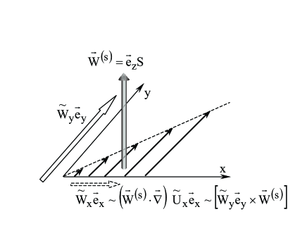
Figure 2: Mechanism for ”skew-induced” generation of perturbations of the mean vorticity $\tilde{W}_{x}$ by quasi-inviscid deflection of the equilibrium mean vorticity $\bar{\bf W}^{(s)}$. In particular, the mean vorticity $\tilde{W}_{x}$ is generated by an interaction of perturbations of the mean vorticity $\tilde{W}_{y}$ and the equilibrium mean vorticity $\bar{\bf W}^{(s)},$ i.e., $\tilde{W}_{x}{\bf e}_{x}\propto(\bar{\bf W}^{(s)}\cdot\mbox{\boldmath$\nabla$})\tilde{U}_{x}{\bf e}_{x}\propto\tilde{W}_{y}{\bf e}_{y}\times\bar{\bf W}^{(s)}.$

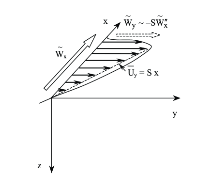
Figure 3: Mechanism for a ”Reynolds stress-induced” generation of perturbations of the mean vorticity $\tilde{W}_{y}$ by turbulent Reynolds stresses. In particular, the mean vorticity $\tilde{W}_{y}$ is generated by an effective anisotropic viscous term $\propto-l_{0}^{2}\,S\,\tilde{W}^{\prime\prime}_{x}$ which is caused by the equilibrium shear motions.

This large-scale instability is similar to a mean-field magnetic dynamo instability (see, e.g., M78 ). Indeed, the first term in Eq. (10) is similar to the differential rotation (or large-scale shear motions) which causes a generation of a toroidal mean magnetic field by a streching of the poloidal mean magnetic field with the differential rotation. On the other hand, the first term in Eq. (11) is similar to the $\alpha$ effect M78 , or to the ”shear-current” effect RK03 . These effects result in generation of a poloidal mean magnetic field from the toroidal mean magnetic field. The $\alpha$-effect is related with the hydrodynamic helicity of an inhomogeneous turbulent flow, while the ”shear-current” effect occurs due to an interaction of the mean vorticity and electric current in a homogeneous anisotropic turbulent flow of a conducting fluid. The magnetic dynamo instability is a combined effect of nonuniform mean flow (differential rotation or large-scale shear motions) and turbulence effects (helical turbulent motions which produce the $\alpha$ effect or anisotropic turbulent motions which cause ”shear-current” effect).

On the other hand, the magnetic dynamo instability is different from the instability of the mean vorticity although they are governed by similar equations. The mean vorticity $\bar{\bf W}=\mbox{\boldmath$\nabla$}{\bf\times}\bar{\bf U}$ is directly determined by the velocity field $\tilde{\bf U},$ while the magnetic field depends on the velocity field through the induction and Navier-Stokes equations.

IV Effect of a mean velocity shear on a turbulence and large-scale instability

In this section we study quantitatively an effect of a mean velocity shear on a turbulence. This allows us to derive an equation for the effective force $\cal F$ and to study the dynamics of the mean vorticity.

IV.1 Method of derivations

To study an effect of a mean velocity shear on a turbulence we used equation for fluctuations ${\bf u}(t,{\bf r})$ which is obtained by subtracting equation for the mean field from the corresponding equation for the total field:

$${\partial{\bf u}\over\partial t} = -(\bar{\bf U}\cdot\mbox{\boldmath$\nabla$}){\bf u}-({\bf u}\cdot\mbox{\boldmath$\nabla$})\bar{\bf U}-{\mbox{\boldmath$\nabla$}p\over\rho}$$ (13)

$$+{\bf F}^{\rm(st)}+{\bf U}_{N}\;,$$

where $p$ are the pressure fluctuations, $\rho$ is the fluid density, ${\bf F}^{\rm(st)}$ is an external stirring force with a zero mean value, and $U_{N}=\langle({\bf u}\cdot\mbox{\boldmath$\nabla$}){\bf u}\rangle-({\bf u}\cdot\mbox{\boldmath$\nabla$}){\bf u}+\nu\Delta{\bf u}.$ We consider a turbulent flow with large Reynolds numbers $({\rm Re}=l_{0}u_{0}/\nu\gg 1).$ We assumed that there is a separation of scales, i.e., the maximum scale of turbulent motions $l_{0}$ is much smaller then the characteristic scale of inhomogeneities of the mean fields. Using Eq. (13) we derived equation for the second moment of turbulent velocity field $f_{ij}({\bf k,R})\equiv\int\langle u_{i}({\bf k}+{\bf K}/2)u_{j}(-{\bf k}+{\bf K}/2)\rangle\exp(i{\bf K}{\bf\cdot}{\bf R})\,d{\bf K}$:

$${\partial f_{ij}({\bf k,R})\over\partial t}=I_{ijmn}(\bar{\bf U})f_{mn}+F_{ij}+f_{ij}^{(N)}\;$$ (14)

(see Appendix B), where

$$I_{ijmn}(\bar{\bf U}) = \biggl{(}2k_{iq}\delta_{mp}\delta_{jn}+2k_{jq}\delta_{im}\delta_{pn}-\delta_{im}\delta_{jq}\delta_{np}$$ (15)

$$-\delta_{iq}\delta_{jn}\delta_{mp}+\delta_{im}\delta_{jn}k_{q}{\partial\over\partial k_{p}}\biggr{)}\nabla_{p}\bar{U}_{q}\;,$$

and ${\bf R}$ and ${\bf K}$ correspond to the large scales, and ${\bf r}$ and ${\bf k}$ to the small scales (see Appendix B), $k_{ij}=k_{i}k_{j}/k^{2},$ $\,f_{ij}^{(N)}({\bf k},{\bf R})$ is the third moment appearing due to the nonlinear term, $\mbox{\boldmath$\nabla$}=\partial/\partial{\bf R},$ $F_{ij}({\bf k},{\bf R})=\langle\tilde{F}_{i}({\bf k},{\bf R})u_{j}(-{\bf k},{\bf R})\rangle+\langle u_{i}({\bf k},{\bf R})\tilde{F}_{j}(-{\bf k},{\bf R})\rangle$ and ${\bf\tilde{F}}({\bf k},{\bf R},t)=-{\bf k}{\bf\times}({\bf k}{\bf\times}{\bf F}^{\rm(st)}({\bf k},{\bf R}))/k^{2}.$ Equation (14) is written in a frame moving with a local velocity $\bar{\bf U}$ of the mean flow. In Eqs. (14) and (15) we neglected small terms which are of the order of $O(|\nabla^{3}\bar{\bf U}|).$ Note that Eqs. (14) and (15) do not contain terms proportional to $O(|\nabla^{2}\bar{\bf U}|).$

The total mean velocity is $\bar{\bf U}=\bar{\bf U}^{(s)}+\tilde{\bf U},$ where we considered a turbulent flow with an imposed mean velocity shear $\nabla_{i}\bar{\bf U}^{(s)}.$ Now let us introduce a background turbulence with zero gradients of the mean fluid velocity $\nabla_{i}\bar{U}_{j}=0.$ The background turbulence is determined by equation $\partial f_{ij}^{(0)}/\partial t=F_{ij}+f_{ij}^{(N0)},$ where the superscript ${(0)}$ corresponds to the background turbulence, and we assumed that the tensor $F_{ij}({\bf k,R}),$ which is determined by a stirring force, is independent of the mean velocity. Equation for the deviations $f_{ij}-f_{ij}^{(0)}$ from the background turbulence is given by

$${\partial(\hat{f}-\hat{f}^{(0)})\over\partial t}=[\hat{I}(\bar{\bf U}^{(s)})+\hat{I}(\tilde{\bf U})]\hat{f}+\hat{f}^{(N)}-\hat{f}^{(N0)}\;,$$ (16)

where we used the following notations: $\hat{f}\equiv f_{ij}({\bf k,R}),$ $\,\hat{f}^{(N)}\equiv f_{ij}^{(N)}({\bf k,R}),$ $\,\hat{f}^{(N0)}\equiv f_{ij}^{(N0)}({\bf k,R}),$ $\,\hat{f}^{(0)}\equiv f_{ij}^{(0)}({\bf k,R}),$ and $\hat{I}(\bar{\bf U})\hat{f}\equiv I_{ijmn}(\bar{\bf U})f_{mn}({\bf k,R}).$

Equation (16) for the deviations of the second moments in ${\bf k}$-space contains the deviations of the third moments and a problem of closing the equations for the higher moments arises. Various approximate methods have been proposed for the solution of problems of this type (see, e.g., MY75 ; O70 ; Mc90 ). The simplest procedure is the $\tau$ approximation which was widely used for study of different problems of turbulent transport (see, e.g., O70 ; PFL76 ; KRR90 ; RK2000 ). One of the simplest procedures, that allows us to express the deviations of the third moments $\hat{f}^{(N)}-\hat{f}^{(N0)}$ in ${\bf k}$-space in terms of that for the second moments $\hat{f}-\hat{f}^{(0)},$ reads

$$\hat{f}^{(N)}-\hat{f}^{(N0)} = -{\hat{f}-\hat{f}^{(0)}\over\tau(k)}\;,$$ (17)

where $\tau(k)$ is the correlation time of the turbulent velocity field. Here we assumed that the time $\tau(k)$ is independent of the gradients of the mean fluid velocity because in the framework of the mean-field approach we may only consider a weak shear: $\tau_{0}|\mbox{\boldmath$\nabla$}\bar{U}|\ll 1,$ where $\tau_{0}=l_{0}/u_{0}.$

The $\tau$-approximation is in general similar to Eddy Damped Quasi Normal Markowian (EDQNM) approximation. However there is a principle difference between these two approaches (see O70 ; Mc90 ). The EDQNM closures do not relax to the equilibrium, and do not describe properly the motions in the equilibrium state. Within the EDQNM theory, there is no dynamically determined relaxation time, and no slightly perturbed steady state can be approached O70 . In the $\tau$-approximation, the relaxation time for small departures from equilibrium is determined by the random motions in the equilibrium state, but not by the departure from equilibrium O70 . Analysis performed in O70 showed that the $\tau$-approximation describes the relaxation to the equilibrium state (the background turbulence) more accurately than the EDQNM approach.

Note that we applied the $\tau$-approximation (17) only to study the deviations from the background turbulence which are caused by the spatial derivatives of the mean velocity. The background turbulence is assumed to be known. Here we used the following model of the background isotropic and homogeneous turbulence:

$$f^{(0)}_{ij}({\bf k},{\bf R}) = \frac{u_{0}^{2}}{8\pi k^{2}}P_{ij}({\bf k}){\cal E}(k)\;,$$ (18)

where $P_{ij}({\bf k})=\delta_{ij}-k_{ij},$ $\,\delta_{ij}$ is the Kronecker tensor, $\tau(k)=2\tau_{0}\bar{\tau}(k),$ $\,{\cal E}(k)=-d\bar{\tau}(k)/dk,$ $\,\bar{\tau}(k)=(k/k_{0})^{1-q},$ $\,1<q<3$ is the exponent of the kinetic energy spectrum (e.g., $q=5/3$ for Kolmogorov spectrum), and $k_{0}=1/l_{0}.$

IV.2 Equation for the second moment of velocity fluctuations

We assume that the characteristic time of variation of the second moment $f_{ij}({\bf k},{\bf R})$ is substantially larger than the correlation time $\tau(k)$ for all turbulence scales. Thus in a steady-state Eq. (16) reads

$$\hat{L}(\hat{f}-\hat{f}^{(0)})=\tau(k)\,[\hat{I}(\bar{\bf U}^{(s)})+\hat{I}(\tilde{\bf U})]\,\hat{f}^{(0)}\;,$$ (19)

where $\hat{L}\equiv L_{ijmn}=\delta_{im}\delta_{jn}-\tau(k)\,[I_{ijmn}(\bar{\bf U}^{(s)})+I_{ijmn}(\tilde{\bf U})],$ and we used Eq. (17). The solution of Eq. (19) yields the second moment $\hat{f}\equiv f_{ij}({\bf k},{\bf R})$:

$$\hat{f} \approx \hat{f}(\bar{\bf U}^{(s)})+\tau(k)\,[\hat{I}(\tilde{\bf U})+\hat{I}(\bar{\bf U}^{(s)})\,\tau(k)\,\hat{I}(\tilde{\bf U})$$ (20)

$$+\hat{I}(\tilde{\bf U})\,\tau(k)\,\hat{I}(\bar{\bf U}^{(s)})]\,\hat{f}^{(0)}\;,$$

where $\hat{f}(\bar{\bf U}^{(s)})=\hat{f}^{(0)}+\tau(k)[\hat{I}(\bar{\bf U}^{(s)})+\hat{I}(\bar{\bf U}^{(s)})\tau(k)\hat{I}(\bar{\bf U}^{(s)})]\hat{f}^{(0)}.$ In Eq. (20) we neglected terms which are of the order of $O(|\nabla\tilde{\bf U}|^{2})$ and $O(\,|\nabla\bar{\bf U}^{(s)}|^{2}|\nabla\tilde{\bf U}|).$ The first term in the equation for $\hat{f}(\bar{\bf U}^{(s)})$ is independent of the mean velocity shear and it describes the background turbulence, while the second and the third terms in this equation determine an effect of the mean velocity shear on turbulence.

IV.3 Effective force

Equation (20) allows us to determine the effective force: ${\cal F}_{i}=-{\nabla}_{j}\int\tilde{f}_{ij}({\bf k},{\bf R})\,d{\bf k},$ where $\tilde{f}=\hat{f}-\hat{f}(\bar{\bf U}^{(s)}),$ and we used notation $\tilde{f}\equiv\tilde{f}_{ij}({\bf k},{\bf R}).$ The integration in ${\bf k}$-space yields the second moment $\tilde{f}_{ij}({\bf R})=\int\tilde{f}_{ij}({\bf k},{\bf R})\,d{\bf k}$:

$$\tilde{f}_{ij}({\bf R}) = -2\nu_{{}_{T}}\,(\partial\tilde{U})_{ij}-l_{0}^{2}\,[4C_{1}\,M_{ij}$$ (21)

$$+C_{2}\,(N_{ij}+H_{ij})+C_{3}\,G_{ij}]\;,$$

where $C_{1}=8(q^{2}-13q+40)/315,$ $\,C_{2}=2(6-7q)/45,$ $\,C_{3}=-2(q+2)/45,$ and the tensors $M_{ij},$ $\,N_{ij},$ $\,H_{ij}$ and $G_{ij}$ are determined by Eqs. (5)-(8). In Eq. (21) we omitted terms $\propto\delta_{ij}$ because they do not contribute to $\mbox{\boldmath$\nabla$}{\bf\times}\mbox{\boldmath$\cal F$}$ (see Eq. (4) for perturbations of the mean vorticity $\tilde{\bf W}).$ To derive Eq. (21) we used the identities presented in Appendix A. Equations (9) and  (21) yield $B_{1}=4C_{1},$ $\,B_{2}=B_{3}=C_{2}$ and $B_{4}=C_{3}.$

Note that the mean velocity gradient $\nabla_{i}\bar{\bf U}^{(s)}$ causes generation of anisotropic velocity fluctuations (tangling turbulence). Inhomogeneities of perturbations of the mean velocity $\tilde{\bf U}$ produce additional velocity fluctuations, so that the Reynolds stresses $\tilde{f}_{ij}({\bf R})$ are the result of a combined effect of two types of velocity fluctuations produced by the tangling of mean gradients $\nabla_{i}\bar{\bf U}^{(s)}$ and $\nabla_{i}\tilde{\bf U}$ by a small-scale Kolmogorov turbulence. Equation (21) allows to determine the effective force ${\cal F}_{i}=-{\nabla}_{j}\tilde{f}_{ij}({\bf R}).$

IV.4 The large-scale instability in a homogeneous turbulence with a mean velocity shear

Let us study the evolution of the mean vorticity using Eq. (21) for the Reynolds stresses. Consider a homogeneous turbulence with a mean velocity shear, e.g., $\bar{\bf U}^{(s)}=(0,Sx,0)$ and $\bar{\bf W}^{(s)}=(0,0,S).$ For simplicity we consider perturbations of the mean vorticity in the form $\tilde{{\bf W}}=(\tilde{W}_{x}(z),\tilde{W}_{y}(z),0).$ Then Eq. (4) reduces to Eqs. (10) and (11), where $\alpha=C_{1}+C_{2}-C_{3}=4(2q^{2}-47q+108)/315,$ and we used Eq. (21). We seek for a solution of Eqs. (10) and (11) in the form $\propto\exp(\gamma t+iKz).$ Thus, the growth rate of perturbations of the mean vorticity is given by $\gamma=\sqrt{\alpha}\,S\,l_{0}\,K-\nu_{{}_{T}}\,K^{2}.$ The maximum growth rate of perturbations of the mean vorticity, $\gamma_{\rm max}=\alpha\,(S\,l_{0})^{2}/4\nu_{{}_{T}}\approx 0.1\,\beta\,S^{2}\tau_{0},$ is attained at $K=K_{m}=\sqrt{\alpha}\,S\,l_{0}/2\nu_{{}_{T}}.$ Here we used that for a Kolmogorov spectrum $(q=5/3)$ of the background turbulence, the factor $\alpha\approx 0.45.$ The sufficient condition $\gamma>0$ for the excitation of the instability reads $L_{W}/l_{0}>2\pi/(\beta\,\sqrt{\alpha}\,\tau_{0}S).$ Since $\tau_{0}S\ll 1$ (we considered a weak velocity shear), the scale $L_{W}\gg l_{0}$ and, therefore, there is a separation of scales. The mechanism of this instability is discussed in Section III and is associated with a combined effect of the ”skew-induced” deflection of equilibrium mean vorticity due to the sheared motions and the ”Reynolds stress-induced” generation of perturbations of mean vorticity.

V Conclusions and applications

We discussed an effect of a mean velocity shear on a turbulence and on the effective force which is determined by the gradient of Reynolds stresses. We demonstrated that in a homogeneous incompressible turbulent flow with an imposed mean velocity shear a large-scale instability can be excited which results in a mean vorticity production. This instability is caused by a combined effect of the large-scale shear motions (”skew-induced” deflection of equilibrium mean vorticity) and ”Reynolds stress-induced” generation of perturbations of mean vorticity. We determined the spatial characteristics, such as the minimum size of the growing perturbations and the size of perturbations with the maximum growth rate.

The analyzed effect of the mean vorticity production may be of relevance in different turbulent industrial, environmental and astrophysical flows (see, e.g., B87 ; BB64 ; P70 ; M84 ; GHW02 ; PA02 ; L83 ; BR98 ; EKR98 ; CH00 ). Thus, e.g., the suggested mechanism can be used in the analysis of the flows associated with the Prandtl’s turbulent secondary flows (see, e.g., B87 ; BB64 ; P70 ; M84 ; GHW02 ; PA02 ). These flows, e.g., arise in straight noncircular ducts, at the lateral boundaries of three-dimensional thin shear layers, etc. The simple model considered in the present paper can mimic the flows associated with turbulent secondary flows.

The obtained results may be also important in astrophysics, e.g., in extragalactic clusters and in interstellar clouds. The extragalactic clusters are nonrotating objects with a homogeneous turbulence in the center of a extragalactic cluster. Sheared motions between interacting clusters can cause an excitation of the large-scale instability which results in the mean vorticity production and formation of large-scale vortices. Dust particles can be trapped by these vortices to enhance agglomeration of material and formation of particles inhomogeneities BR98 ; EKR98 ; CH00 . The sheared motions can also occur between interacting interstellar clouds, whereby the dynamics of the mean vorticity is important.

Appendix A Identities used for derivation of Eqs. (10), (11) and (21)

To derive Eqs. (10) and (11) we used the following identities:

$$\mbox{\boldmath$\nabla$}{\bf\times}{\bf M} = (SK^{2}/4)(\tilde{W}_{y},\tilde{W}_{x},0)\;,$$

$$\mbox{\boldmath$\nabla$}{\bf\times}(\tilde{\bf U}{\bf\times}\bar{\bf W}^{(s)}) = S(\tilde{W}_{y},-\tilde{W}_{x},0)\;,$$

$$\mbox{\boldmath$\nabla$}{\bf\times}(\bar{\bf U}^{(s)}{\bf\times}\tilde{\bf W}) = S(0,\tilde{W}_{x},0)\;,$$

$$\mbox{\boldmath$\nabla$}{\bf\times}{\bf J} = (SK^{2}/2)(\tilde{W}_{y},\tilde{W}_{x},0)\;,$$

$$\mbox{\boldmath$\nabla$}{\bf\times}[(\bar{\bf W}^{(s)}\cdot\mbox{\boldmath$\nabla$})\tilde{\bf W}] = SK^{2}(\tilde{W}_{y},-\tilde{W}_{x},0)\;,$$

where $M_{i}=\nabla_{j}M_{ij},$ $J_{i}=\nabla_{j}[\tilde{W}_{n}(\varepsilon_{nim}(\partial\bar{U}^{(s)})_{mj}+\varepsilon_{njm}(\partial\bar{U}^{(s)})_{mi})],$ and we also took into account that

$$\nabla_{j}G_{ij}=(\bar{\bf W}^{(s)}\cdot\mbox{\boldmath$\nabla$})\tilde{W}_{i}\;,$$

$$\nabla_{j}[\bar{W}^{(s)}_{n}(\varepsilon_{nim}(\partial\tilde{U})_{mj}+\varepsilon_{njm}(\partial\tilde{U})_{mi})]$$

$$=[\nabla_{i}(\bar{\bf W}^{(s)}\cdot\tilde{\bf W})-(\bar{\bf W}^{(s)}\cdot\mbox{\boldmath$\nabla$})\tilde{W}_{i}]/2\;.$$

To derive Eq. (21) we used the following identities for the integration over the angles in ${\bf k}$-space:

$$\int k_{ijmn}\,d\hat{\Omega}={4\pi\over 15}\Delta_{ijmn}\;,$$

$$T_{ijmnpq}\equiv\int k_{ijmnpq}\,d\hat{\Omega}={4\pi\over 105}(\Delta_{mnpq}\delta_{ij}$$

$$+\Delta_{jmnq}\delta_{ip}+\Delta_{imnq}\delta_{jp}+\Delta_{jmnp}\delta_{iq}$$

$$+\Delta_{imnp}\delta_{jq}+\Delta_{ijmn}\delta_{pq}-\Delta_{ijpq}\delta_{mn})\;,$$

$$T_{ijmnpq}(\nabla_{m}\bar{U}^{(s)}_{n})(\nabla_{p}\tilde{U}_{q})={4\pi\over 105}(4M_{ij}+\delta_{ij}M_{pp})\;,$$

$k_{ijmn}=k_{i}k_{j}k_{m}k_{n}/k^{4},$ $\,d\hat{\Omega}=\sin\theta\,d\theta\,d\varphi,$ $\,k_{ijmnpq}=k_{ijmn}k_{pq}$ and $\Delta_{ijmn}=\delta_{ij}\delta_{mn}+\delta_{im}\delta_{nj}+\delta_{in}\delta_{mj}.$

Appendix B Derivation of Eq. (14)

In order to derive Eq. (14) we use a two-scale approach, i.e., a correlation function is written as follows

$$\langle u_{i}({\bf x})u_{j}({\bf y})\rangle = \int\langle u_{i}({\bf k}_{1})u_{j}({\bf k}_{2})\rangle\exp[i({\bf k}_{1}{\bf\cdot}{\bf x}$$

$$+{\bf k}_{2}{\bf\cdot}{\bf y})]\,d{\bf k}_{1}\,d{\bf k}_{2}$$

$$= \int f_{ij}({\bf k,R})\exp(i{\bf k}{\bf\cdot}{\bf r})\,d{\bf k}\;,$$

$$f_{ij}({\bf k,R}) = \int\langle u_{i}({\bf k}+{\bf K}/2)u_{j}(-{\bf k}+{\bf K}/2)\rangle$$

$$\times\exp(i{\bf K}{\bf\cdot}{\bf R})\,d{\bf K}\;$$

(see, e.g., RS75 ; KR94 ), where ${\bf R}$ and ${\bf K}$ correspond to the large scales, and ${\bf r}$ and ${\bf k}$ to the small scales, i.e., ${\bf R}=({\bf x}+{\bf y})/2,$ $\quad{\bf r}={\bf x}-{\bf y},$ $\quad{\bf K}={\bf k}_{1}+{\bf k}_{2},$ $\quad{\bf k}=({\bf k}_{1}-{\bf k}_{2})/2.$ This implies that we assumed that there exists a separation of scales, i.e., the maximum scale of turbulent motions $l_{0}$ is much smaller then the characteristic scale of inhomogeneities of the mean fields.

Now we calculate

$${\partial f_{ij}({\bf k}_{1},{\bf k}_{2})\over\partial t} \equiv \langle P_{in}({\bf k}_{1}){\partial u_{n}({\bf k}_{1})\over\partial t}u_{j}({\bf k}_{2})\rangle$$ (22)

$$+\langle u_{i}({\bf k}_{1})P_{jn}({\bf k}_{2}){\partial u_{n}({\bf k}_{2})\over\partial t}\rangle\;,$$

where we multiplied equation of motion (13) rewritten in ${\bf k}$-space by $P_{ij}({\bf k})=\delta_{ij}-k_{ij}$ in order to exclude the pressure term from the equation of motion, $\delta_{ij}$ is the Kronecker tensor and $k_{ij}=k_{i}k_{j}/k^{2}.$ Thus, the equation for $f_{ij}({\bf k,R})$ is given by Eq. (14).

For the derivation of Eq. (14) we used the following identity

$$ik_{i}\int f_{ij}({\bf k}-{1\over 2}{\bf Q},{\bf K}-{\bf Q})\bar{U}_{p}({\bf Q})\exp(i{\bf K}{\bf\cdot}{\bf R})\,d{\bf K}\,d{\bf Q}$$

$$=-{1\over 2}\bar{U}_{p}\nabla_{i}f_{ij}+{1\over 2}f_{ij}\nabla_{i}\bar{U}_{p}-{i\over 4}(\nabla_{s}\bar{U}_{p})\biggl{(}\nabla_{i}{\partial f_{ij}\over\partial k_{s}}\biggr{)}$$

$$+{i\over 4}\biggl{(}{\partial f_{ij}\over\partial k_{s}}\biggr{)}(\nabla_{s}\nabla_{i}\bar{U}_{p})\;.$$ (23)

To derive Eq. (23) we multiply the equation $\mbox{\boldmath$\nabla$}~{}\cdot~{}{\bf u}=0,$ written in ${\bf k}$-space for $u_{i}({\bf k}_{1}-{\bf Q}),$ by $u_{j}({\bf k}_{2})\bar{U}_{p}({\bf Q})\exp(i{\bf K}{\bf\cdot}{\bf R}),$ and integrate over ${\bf K}$ and ${\bf Q}$, and average over ensemble of velocity fluctuations. Here ${\bf k}_{1}={\bf k}+{\bf K}/2$ and ${\bf k}_{2}=-{\bf k}+{\bf K}/2.$ This yields

$$\int i\biggl{(}k_{i}+{1\over 2}K_{i}-Q_{i}\biggr{)}\langle u_{i}({\bf k}+{1\over 2}{\bf K}-{\bf Q})u_{j}(-{\bf k}+{1\over 2}{\bf K})\rangle$$

$$\times\bar{U}_{p}({\bf Q})\exp{(i{\bf K}{\bf\cdot}{\bf R})}\,d{\bf K}\,d{\bf Q}=0\;.$$ (24)

Next, we introduce new variables: $\tilde{\bf k}_{1}={\bf k}+{\bf K}/2-{\bf Q},$ $\tilde{\bf k}_{2}=-{\bf k}+{\bf K}/2$ and $\tilde{\bf k}=(\tilde{\bf k}_{1}-\tilde{\bf k}_{2})/2={\bf k}-{\bf Q}/2,$ $\tilde{\bf K}=\tilde{\bf k}_{1}+\tilde{\bf k}_{2}={\bf K}-{\bf Q}.$ This allows us to rewrite Eq. (24) in the form

$$\int i\biggl{(}k_{i}+{1\over 2}K_{i}-Q_{i}\biggr{)}f_{ij}({\bf k}-{1\over 2}{\bf Q},{\bf K}-{\bf Q})\bar{U}_{p}({\bf Q})$$

$$\times\exp{(i{\bf K}{\bf\cdot}{\bf R})}\,d{\bf K}\,d{\bf Q}=0\;.$$ (25)

Since $|{\bf Q}|\ll|{\bf k}|$ we can use the Taylor expansion

$$f_{ij}({\bf k}-{\bf Q}/2,{\bf K}-{\bf Q})\simeq f_{ij}({\bf k},{\bf K}-{\bf Q})$$

$$-\frac{1}{2}{\partial f_{ij}({\bf k},{\bf K}-{\bf Q})\over\partial k_{s}}Q_{s}+O({\bf Q}^{2})\;.$$ (26)

We also use the following identities:

$$[f_{ij}({\bf k},{\bf R})\bar{U}_{p}({\bf R})]_{\bf K}=\int f_{ij}({\bf k},{\bf K}-{\bf Q})\bar{U}_{p}({\bf Q})\,d{\bf Q}\;,$$

$$\nabla_{p}[f_{ij}({\bf k},{\bf R})\bar{U}_{p}({\bf R})]=\int iK_{p}[f_{ij}({\bf k},{\bf R})\bar{U}_{p}({\bf R})]_{\bf K}$$

$$\times\exp{(i{\bf K}{\bf\cdot}{\bf R})}\,d{\bf K}\;.$$ (27)

Therefore, Eqs. (25)-(27) yield Eq. (23).

References

• (1) L. Prandtl, Essentials of Fluid Dynamics (Blackie, London, 1952).
• (2) A. A. Townsend, The Structure of Turbulent Shear Flow (Cambridge Univ. Press, Cambridge, 1956).
• (3) P. Bradshaw, Ann. Rev. Fluid Mech. 19, 53 (1987), and references therein.
• (4) E. Brundrett and W. D. Baines, J. Fluid Mech. 19, 375 (1964).
• (5) H. J. Perkins, J. Fluid Mech. 44, 721 (1970).
• (6) B. R. Morton, Geophys. Astrophys. Fluid Dyn. 28, 277 (1984).
• (7) L. M. Grega, T. Y. Hsu and T. Wei, J. Fluid Mech. 465, 331 (2002).
• (8) B. A. Pettersson Reif and H. I. Andersson, Flow, Turbulence and Combustion 68, 41 (2002).
• (9) A. J. Chorin, Vorticity and Turbulence (Springer, New York, 1994), and references therein.
• (10) A. Tsinober, Eur. J. Mech. B/Fluids 17, 421 (1998).
• (11) C. Reyl, T. M. Antonsen and E. Ott, Physica D 111, 202 (1998).
• (12) J. Pedlosky, Geophysical Fluid Dynamics (Springer, New York, 1987), and references therein.
• (13) A. Glasner, E. Livne and B. Meerson, Phys. Rev. Lett. 78, 2112 (1997).
• (14) H. K. Moffatt, Magnetic Field Generation in Electrically Conducting Fluids (Cambridge University Press, New York, 1978), and references therein.
• (15) I. Rogachevskii and N. Kleeorin, Phys. Rev. E, submitted (2003).
• (16) T. Elperin, N. Kleeorin, I. Rogachevskii and S. S. Zilitinkevich, Phys. Rev. E 66, 066305 (2002).
• (17) A. D. Wheelon, Phys. Rev. 105, 1706 (1957).
• (18) G. K. Batchelor, I. D. Howells and A. A. Townsend, J. Fluid Mech. 5, 134 (1959).
• (19) G. S. Golitsyn, Doklady Acad. Nauk 132, 315 (1960) [Soviet Phys. Doklady 5, 536 (1960)].
• (20) H. K. Moffatt, J. Fluid Mech. 11, 625 (1961).
• (21) J. L. Lumley, Phys. Fluids, 10 1405 (1967).
• (22) J. C. Wyngaard and O. R. Cote, Q. J. R. Meteorol. Soc. 98, 590 (1972).
• (23) S. G. Saddoughi and S. V. Veeravalli, J. Fluid Mech. 268, 333 (1994).
• (24) T. Ishihara, K. Yoshida and Y. Kaneda, Phys. Rev. Lett. 88, 154501 (2002).
• (25) S. A. Orszag, J. Fluid Mech. 41, 363 (1970), and references therein.
• (26) A. S. Monin and A. M. Yaglom, Statistical Fluid Mechanics (MIT Press, Cambridge, Massachusetts, 1975), and references therein.
• (27) W. D. McComb, The Physics of Fluid Turbulence (Clarendon, Oxford, 1990).
• (28) A. Pouquet, U. Frisch, and J. Leorat, J. Fluid Mech. 77, 321 (1976).
• (29) N. Kleeorin, I. Rogachevskii, and A. Ruzmaikin, Sov. Phys. JETP 70, 878 (1990); N. Kleeorin, M. Mond, and I. Rogachevskii, Astron. Astrophys. 307, 293 (1996).
• (30) I. Rogachevskii and N. Kleeorin, Phys. Rev. E 61, 5202 (2000); 64, 056307 (2001).
• (31) H.J. Lugt, Vortex Flow in Nature and Technology (J. Wiley and Sons, New York, 1983), and references therein.
• (32) L.S. Hodgson and A. Brandenburg, Astron. Astrophys. 330, 1169 (1998).
• (33) T. Elperin, N. Kleeorin and I. Rogachevskii, Phys. Rev. Lett. 81, 2898 (1998).
• (34) P.H. Chavanis, Astron. Astrophys. 356, 1089 (2000).
• (35) P. N. Roberts and A. M. Soward, Astron. Nachr. 296, 49 (1975).
• (36) N. Kleeorin and I. Rogachevskii, Phys. Rev. E 50, 2716 (1994).