Non-Gaussianity: Comparing wavelet and Fourier based methods

In the context of the present and future Cosmic Microwave Background (CMB) experiments, going beyond the information provided by the power spectrum has become necessary in order to tightly constrain the cosmological model. The non-Gaussian signatures in the CMB represent a very promising tool to probe the early universe and the structure formation epoch. We present the results of a comparison between two families of non-Gaussian estimators: The first act on the wavelet space (skewness and excess kurtosis of the wavelet coefficients) and the second group on the Fourier space (bi- and trispectrum). We compare the relative sensitivities of these estimators by applying them to three different data sets meant to reproduce the majority of possible non-Gaussian contributions to the CMB. We find that the skewness in the wavelet space is slightly more sensitive than the bispectrum. For the four point estimators, we find that the excess kurtosis of the wavelet coefficients has very similar capabilities than the diagonal trispectrum while a near-diagonal trispectrum seems to be less sensitive to non-Gaussian signatures.

1 Introduction

Over the last few years, the amount of available data on the Cosmic Microwave Background (CMB) has increased dramatically. Recent measurements of the CMB power spectrum (BOOMERANG, MAXIMA, DASI, CBI, ARCHEOPS, VSA, ACBAR…) have started to shed light on the origin and large scale structure of our universe. In particular, the determination of the density parameter $\Omega\simeq 1$ has been obtained from the position of the first acoustic peak. Together with results from other experiments, which probe e.g. the distribution of galaxies and the distances to type-Ia supernovae, a coherent image of todays universe has started to emerge (see e.g. Wang et al. (2002)). Testing the detailed statistical nature of the CMB anisotropies has become not only one of the major goals of CMB cosmology but it is now also within our reach. The MAP satellite (and also the future Planck mission) will provide us with an all sky survey of the CMB with good angular resolution that can be used to search for non-Gaussian signatures.

A Gaussian random field is completely determined by its power spectrum. But many models of the early universe, like inflation (e.g. Bartolo et al. (2002), Bernardeau & Uzan (2002) and references therein), super strings or topological defects, predict non-Gaussian contributions to the initial fluctuations Luo (1994b); Jaffe (1994); Gangui et al. (1994). Furthermore, any non-linearity in their evolution introduces additional non-Gaussian signatures. An extreme example is gravitational clustering, which makes it quite difficult to extract any primordial non-Gaussianity from the galaxy distribution Durrer et al. (2000). The CMB on the other hand is to first order free of this complication and is therefore ideally suited to study the early universe. Nevertheless, secondary effects like the Sunyaev-Zel’dovich (SZ) effect Aghanim & Forni (1999); Cooray (2001), the Ostriker-Vishniac effect Castro (2002), lensing Cooray & Hu (2001); Bernardeau et al. (2002) and others add their own contributions to the total non-Gaussianity. To these cosmological effects, we have to add foregrounds as well as systematic effects and instrumental noise. In order to disentangle all those sources from one another, it is essential to assemble a “tool-box” of well-understood, fast and robust methods for probing different aspects of the non-Gaussian signatures.

In this paper, we compare the behaviour of two different classes of estimators, namely the higher order moments in wavelet space, and the bi- and trispectrum. Both of these do not act directly on pixels, but are applied in a dual space. The purpose of this study is not to present novel ways of detecting non-Gaussian signatures, but to discuss practical aspects of these different approaches, and to compare their behaviour when applied to a selection of synthetic “benchmark” maps which are designed to mimic typical non-Gaussian contributions to the CMB.

After the seminal work of Pando et al. (1998) which consisted of applying wavelet techniques to look for non-Gaussian signatures in the COBE-DMR data, several methods based on the wavelet analysis have been developed in the context of the CMB detection of non-Gaussian signatures Aghanim & Forni (1999); Forni & Aghanim (1999); Hobson et al. (1999); Barreiro & Hobson (2001); Cayon et al. (2001); Jewell (2001); Martinez-Gonzalez et al. (2002); Starck et al. (2003). These methods have proven particularly suitable for statistical studies due to the combination of two characteristics. First, wavelets are quite localised both in space and in frequency, which allows for the features of interest in an image to be present at different scales. Second, the linear transformation properties of Gaussian variables preserve Gaussianity. Conversely, any non-Gaussian signal will exhibit a non-Gaussian distribution of its wavelet coefficients. The two properties combined together allow us to associate the statistical signatures with the spatial features that have caused them.

The wavelet based estimators have been tested and qualified in terms of their sensitivity to the non-Gaussian signatures on a variety of simulated data sets such as cosmic strings, the SZ effect from galaxy clusters, and anisotropies from inhomogeneous reionisation (see the above mentioned references). Also the galactic contamination from dust emission can induce foreground non-Gaussian signatures. Wavelets have been used in such a context by Jewell (2001) to quantify the predicted level of non-Gaussian features in the IRAS maps. Additionally, the wavelet based non-Gaussian analysis has also been applied to the COBE-DMR maps.

Different decomposition schemes and wavelet bases can be used for the non-Gaussian studies. In the following, we use a bi-orthogonal wavelet basis and a dyadic decomposition scheme. This choice has been first motivated in Forni & Aghanim (1999) and Aghanim & Forni (1999) by the fact that it is the best scheme in the context of statistical analysis of CMB signals. It is indeed optimal for statistics since it gives, at each scale, the maximum number of significant coefficients. In addition, it naturally allows us to benefit from spatial correlations in the signal at each scale. The better performances of the bi-orthogonal dyadic wavelet decomposition were confirmed by Barreiro & Hobson (2001), and also more recently by Starck et al. (2003), in a comparison with the “à trous” and ridgelet decompositions.

We now focus on the Fourier based analysis. The interest in using higher order correlation functions to study non-Gaussianity dates back many years Luo (1994a); Jaffe (1994); Heavens (1998). The first detection of a non-Gaussian contribution in real CMB data was achieved using the bispectrum Ferreira et al. (1998), but later shown to be due to a weak systematic effect Banday et al. (2000).

Numerous works deal with the construction of ideal higher order statistical estimators both in spherical and flat space as well as with their application to real data (CMB and large-scale structure survey data). In the CMB context, research focused on the two first higher order correlation functions in Fourier space, namely the bispectrum (see recent work by Santos et al. (2002) and citations therein), and its 4-point equivalent, the trispectrum (see Hu (2001); Kunz et al. (2001); Cooray & Kesden (2002)). An important advantage of $n$-point functions over other non-Gaussian statistics such as wavelets or Minkowski functionals is that they are easier to predict for inflation but also for secondary sources. This makes them a very powerful test, explaining their interest for the scientific community.

Indeed, the Boltzmann equation, which describes the time evolution of the perturbations in the cosmic fluid, does not mix different Fourier modes. The structure of linear perturbations is therefore generally simple in Fourier space. Furthermore, the projection of the CMB photons onto the sky sphere is simple as well, with the square of the spherical Bessel functions coupling the Fourier mode $k$ and the angular scale, or more directly the multipole $\ell$, on the sphere. The success of studying the angular power spectrum $C_{\ell}$ lies in that much of the initial conditions is preserved throughout the evolution. Higher order correlation functions can be treated in much the same way and allow for the use of already existing techniques. It is therefore feasible to predict theoretically the expected contributions to non-Gaussian signatures from different sources. This allows us on the one hand to place limits on sources of non-Gaussian features if none is detected, and on the other hand might enable us to solve the inverse problem, namely identifying the origin of the non-Gaussianity, if any is found.

In this work, we concentrate on the flat space approach. We use a normalised bispectrum probing all the possible triangle configurations which exist in a homogeneous and isotropic universe, and a normalised diagonal as well as nearly-diagonal trispectrum which depends on the side and the diagonal of the (nearly) trapezoidal configuration. These are supposed to give us information on the scale dependence of any non-Gaussian signal, but contrary to the wavelets, no spatial position information is retained.

We will start in the next section by presenting the data sets used for the comparison. In section 3, we examine the estimators of the non-Gaussian signatures. The statistical analysis and the results are presented in section 4. We then end with our main conclusions.

2 Data sets

We test the statistical methods to detect non-Gaussian signals on three different data sets chosen so that they are representative of many astrophysical situations. It is beyond the scope of the present study to characterise the astrophysical processes represented by the maps. The three sets have rather to be considered as test cases used in order to insure that the non-Gaussian detection is neither specific to one peculiar type of non-Gaussian signatures, nor due to one particular detection method. Additionally, the combination of the different detection techniques on the different sets of data allows us to compare the relative sensitivities of the methods on an objective basis.

In practise, many of the astrophysical situations can be roughly classified into the following three different types of signals: i) spherically shaped structures standing for compact astrophysical sources or beam-convolved point sources (e.g. galaxies, galaxy clusters) that we refer to as the point sources, ii) strongly anisotropic structures that represent filaments and elongated structures (e.g. interstellar clouds) that we refer to as the filaments, and iii) non-linear couplings leading to non-Gaussian signatures, referred to as the $\chi^{2}$ (or $\chi$-squared) map, as we use the superposition of a Gaussian random field and its square.

In order to characterise the non-Gaussian signatures exhibited by all these signals, the maps are compared to a set of 99 Gaussian realisations having the same power spectrum, referred to as the Gaussian reference set. Therefore, the only difference between Gaussian and non-Gaussian sets is due to the statistical nature of the two processes. All the maps (Gaussian and non-Gaussian) are composed of $500\times 500$ pixels of 1.5 arc minutes aside.

2.1 Filaments

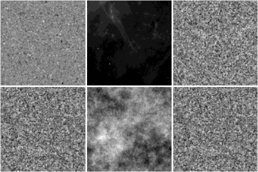
The set of maps for the filamentary structures is a selection of 28 IRAS maps which represent the galactic dust emission at high latitudes. These maps were chosen on the basis of their visual aspect so that they exhibit large and bright filaments (Fig. 1, upper middle panel). Therefore, they all have a low amount of point sources and they exhibit elongated structures. In order to focus on the statistical properties of the maps, the selection has also been made on the basis of their power spectrum. We choose the maps showing power spectra with similar shapes regardless of their amplitudes. We then modify the initial IRAS maps so that their power spectra are rescaled. Figure 2, lower panel, shows the power spectrum of the filaments. Thanks to this rescaling, we can consider the 28 modified IRAS maps as statistical realisations of the same highly non-Gaussian process. This data set has a skewness (third moment) of $0.89\pm 0.34$ ($1\,\sigma$), the excess kurtosis (fourth moment) is $2.63\pm 2.42$. The Gaussian reference maps (one example is given Fig. 1, lower middle panel) have a skewness of $-0.01\pm 0.17$ and an excess kurtosis of $-0.11\pm 0.19$. The large fluctuations of the skewness and excess kurtosis (also present in the Gaussian maps) arise due to the high power on large scales associated with the large structures in the IRAS maps. Hence, even the maps produced using a Gaussian random process could be easily mistaken as being non-Gaussian, proving the necessity of comparing a given test map with a set of Gaussian reference maps with the same power spectrum, rather than relying on a theoretical prediction of the Gaussian bounds. For a discussion of the Gaussian reference maps, see section 2.4.

Figure 1: Representative maps of the non-Gaussian signals and one of their associated Gaussian realisations with the same power spectrum. Upper and lower left panels represent respectively a point source map and one Gaussian realisation. The upper and lower middle panels are for the filaments and an associated Gaussian realisation. The upper and lower right panels represent the $\chi^{2}$ map and a Gaussian field with the same power spectrum.

2.2 Point source maps

The second data set is referred to as the point sources. It is constituted of 50 simulated maps which consist of a distribution of Gaussian shaped sources having different sizes and amplitudes. They are randomly distributed on the map and have positive and negative signs (see Fig. 1, left upper panel). This signal is aimed at reproducing the typical situation of a crowded field of 12.5 square degrees containing $\simeq 10^{7}$ sources. The field therefore exhibits obvious confusion effects. All the simulated maps have the same bell-shaped power spectrum (Fig. 2, upper panel) and exhibit a non-Gaussian signal. This non-Gaussian data set has a skewness of $-0.160\pm 0.078$ and an excess kurtosis of $2.19\pm 0.32$. A Gaussian reference set of maps with the same power spectrum is simulated (Sect. 2.4, Fig. 1, left lower panel). The corresponding Gaussian maps have a skewness of $-0.003\pm 0.022$ and an excess kurtosis of $-0.005\pm 0.036$. The point source maps are hence clearly marked as being non-Gaussian by their excess of kurtosis.

Figure 2: The power spectra of the studied signals in arbitrary units. The upper panel shows the power spectrum of both the point sources and the $\chi^{2}$ maps. The lower panel represents the power spectrum of the filaments.

2.3 $\chi$-squared maps

The two previously described types of non-Gaussian signals are ideal to model astrophysical induced non-linearities due to foregrounds and/or secondary effects. However in a wider context, we can expect the existence of primordial sources of non-Gaussian signatures. A way of modelling some of these signatures is by introducing a non-linear coupling in an originally Gaussian distributed perturbation field Coles & Barrow (1987); Komatsu & Spergel (2000); Bartolo et al. (2002). The simplest weak non-linear coupling is given by $\chi({\mathbf{x}})=\chi_{L}({\mathbf{x}})+f_{NL}(\chi_{L}^{2}({\mathbf{x}})-<\chi_{L}^{2}({\mathbf{x}})>)$, where $\chi_{L}$ denotes the original linear Gaussian field. The non-Gaussian signature introduced by the coupling is quantified by the so-called non-linear coupling constant $f_{NL}$ (note that $<\chi({\mathbf{x}})>=0$).

To generate these $\chi^{2}$ maps we use a method similar to the one followed to create a Gaussian distributed field (see section 2.4). The non-Gaussian character is introduced by adding to the white noise field its squared minus its squared average weighted by $f_{NL}$. When multiplying the non-linear field in Fourier space with the desired power spectrum, a normalisation by $1+2f^{2}_{NL}$ is needed in order to recover the power spectrum from the final map. In our approach, $f_{NL}$ quantifies the amount of the $\chi^{2}$ type contribution in the Gaussian map.

We compute two sets of $50$ maps for $f_{NL}=0.01$ and $0.1$ in order to test the sensitivity of the statistical methods to the amount of non-Gaussian signal introduced in the Gaussian field. For illustration purposes, we show in Fig. 1 right upper and lower panels a $\chi^{2}$ map for $f_{NL}=0.01$ and one associated Gaussian realisation. The power spectrum of these maps was chosen arbitrarily to be the same as for the point source maps. As mentioned before, these maps are not meant to reproduce accurately the physical processes – to simulate a “real” CMB map with a primordial $\chi^{2}$ contribution we would need to integrate over the radiation transfer function. Nevertheless, to relate the order of magnitude of our numbers to the ones found in the literature, we note that they are rescaled by approximately a factor of $\Phi\sim\Delta T/T\sim 10^{-5}$ so that a value of $f_{NL}=0.01$ here corresponds to about $f_{NL}\approx 1000$ elsewhere (in reality a bit less, since e.g. on large scales $\Delta T/T\approx\Phi/3$). The $\chi$-squared maps with $f_{NL}=0.01$ have a skewness of $0.009\pm 0.019$ and an excess kurtosis of $0.002\pm 0.031$, both of which are consistent with zero. The maps with $f_{NL}=0.1$ on the other hand have a skewness of $0.140\pm 0.024$ and an excess kurtosis of $0.037\pm 0.036$. The Gaussian reference set is the same as for the point source maps, see section 2.2.

2.4 Gaussian realisations

In the process of investigating the statistical character of non-Gaussian signals, as we always deal with a finite ensemble of maps, there can be substantial fluctuations in the results (see for example the IRAS case, section 2.1). Furthermore, although not important in our case but rather when analysing experimental data, often a “Gaussian” map is not created directly from a pure Gaussian random process, but has super-imposed known systematic effects (which would result in spurious non-Gaussian features). In general, the output of an estimator applied to a test-map is therefore not compared to a theoretical result but to the corresponding output obtained from a set of Gaussian reference maps (with any known systematic effects one may need to add). Any detection of non-Gaussian signatures can then be reliably quantified by comparing these two sets of results, and we discuss this procedure in section 4.1 in more detail.

We generate two sets of Gaussian distributed fields with the power spectrum of the corresponding non-Gaussian set. The first one is the aforementioned reference set. The second one (called the Gaussian counterpart set) is strictly speaking redundant, but is used to illustrate the fluctuations arising from finite ensembles, and the presence of low-probability results which appear even when comparing Gaussian maps with each other if many different tests are applied.

The simplest standard method Peacock (1999) is to create a spatial array of white noise using a random number generator with zero mean and unit variance. We can then give this Gaussian field the desired power spectrum by multiplying it in Fourier space with the square root of that power spectrum, the one of the non-Gaussian set in our case. Using this procedure, we compute one set of 149 Gaussian maps (reference set and counterparts) with the same power spectrum as the 50 point-source maps, one set of 127 Gaussian maps (reference set and counterparts) with the same power spectrum as the 28 IRAS modified maps. We arbitrarily choose the power spectrum of the point source maps for the $\chi^{2}$ maps and hence use the same set of Gaussian realisations. We show in Fig. 1 (lower panels) one representative Gaussian realisation for each data set with the same spectrum as the non-Gaussian map. The skewness and the excess kurtosis of all the Gaussian reference sets and counterparts are expected to be zero. However, in practice they have a finite scatter. The lower limit for the standard deviation of the skewness is given for a normal distribution with unit variance by $\sqrt{15/N^{2}}$, or about $0.0077$ in the case of $N^{2}=500^{2}$ independent values per map. The expected standard deviation for the excess kurtosis, in the same idealised case, is $\sqrt{96/N^{2}}$ or $0.020$. One should note however that the scatter of higher order moments is much larger in realistic cases and is strongly susceptible to the details of the random process (see sections 2.1, 2.2 and 2.3 for the actual numbers for the Gaussian reference sets).

3 Estimators of the non-Gaussian signatures

We examine two large families of estimators for non-Gaussian signatures. Both are based on dual space analysis. On the one hand, we focus on methods which are completely defined in Fourier space (namely the bi- and trispectrum). On the other hand, we study estimators in the wavelet space (namely third and fourth moments of the wavelet coefficients) in which signals are located both in pixel and in frequency space. It is worth noting that the skewness (third moment) and excess kurtosis (fourth moment) of the wavelet coefficients are quite similar to respectively the bi- and trispectrum, in Fourier space. Additionally, we compute the cumulative probability function (CPF) of the pixel distribution. This latter is also one of the Minkowski functionals, often called $\cal{A}$, the surface of the excursion set at a given amplitude. As the CPF is a less powerful non-Gaussian estimator, in the sense that it does not give information on the scales nor on the physical location of any detection, we intend to use it only as a baseline for the detection of non-Gaussian signatures on a given map.

As discussed above, we analyse a certain number $N_{\mathrm{N}G}$ of non-Gaussian as well as Gaussian maps with the same power spectrum and compare their properties to a reference set of 99 Gaussian realisations, also with the same power spectrum. This section describes the statistical estimators we use for our analysis. For a discussion of the tools used to interpret the results, see section 4.1.

3.1 Pixel distribution function in real space

As we have seen, in the Gaussian case each pixel is an independent realisation of a Gaussian random process. Therefore, one of the easiest and most direct tests of the Gaussian hypothesis just estimates the cumulative probability function (CPF) from the ensemble of pixels $N_{\rm tot}$. To this end, we set

$$P(<x)=N[{\rm pixels\leavevmode\nobreak\ with\leavevmode\nobreak\ values}<x]/N_{\rm tot}.$$ (1)

Since we have several independent maps for both the Gaussian as well as the non-Gaussian processes, we can improve our estimate of the CPF, and hence the sensitivity of the test, by just combining the pixels from all maps. The two CPFs (from the Gaussian and non-Gaussian processes) can then be compared with statistical methods detailed in section 4.1.

Power spectra which vary extremely rapidly (like the ones used here) can strongly amplify the random fluctuations. In this case, the KS test will lead to spurious detections of non-Gaussianity even for Gaussian maps (see e.g. Aghanim & Forni (1999)). It is therefore best to “whiten” the maps first, by deconvolving them with their estimated power spectrum.

Due to its simplicity and its inherent locality (the CPF does not test the relative position or configuration of the fluctuations, as the location of the pixels in the map is not taken into account), and as stated previously, we use the CPF method as a baseline for the comparison between the non-Gaussian methods. It should be stressed clearly that this test can only detect non-Gaussian signatures but does not give any further information about their location or scale dependence. It can therefore only very weakly distinguish between different non-Gaussian contributions.

3.2 Wavelet space analysis

The principle behind the wavelet transform Grossman & Morlet (1984); Daubechies (1988); Mallat (1989) is to hierarchically decompose an input signal into a series of successively lower resolution reference signals and associated detail signals. At each decomposition level, $j$, the reference signal has a resolution reduced by a factor of $2^{j}$ with respect to the original signal. Together with its respective detail signal, each scale contains the information needed to reconstruct the reference signal at the next higher resolution level.

The wavelet analysis can be considered as a series of bandpass filters. It can thus be viewed as the decomposition of the signal in a set of independent, spatially oriented frequency channels. Using the orthogonality properties, a function in this decomposition can be completely characterised by the wavelet basis and the wavelet coefficients in this decomposition.

The multi-level wavelet transform (analysis stage) decomposes the signal into sets of different frequency bands by iterative application of a pair of Quadrature Mirror Filters (QMF). A scaling function and a wavelet function are associated with this analysis filter bank. The continuous scaling function $\phi_{\mathrm{A}}(x)$ satisfies the following two-scale equation:

$$\phi_{\mathrm{A}}(x)=\sqrt{2}\sum_{n}h_{0}(n)\phi_{\mathrm{A}}(2x-n),$$ (2)

where $h_{0}$ is the low-pass QMF. The continuous wavelet $\psi_{\mathrm{A}}(x)$ is defined in terms of the scaling function and the high-pass QMF $h_{1}$ through:

$$\psi_{\mathrm{A}}(x)=\sqrt{2}\sum_{n}h_{1}(n)\phi_{\mathrm{A}}(2x-n).$$ (3)

The same relations apply for the inverse transform (synthesis stage) but, generally, different scaling and wavelet functions ($\phi_{\mathrm{S}}(x)$ and $\psi_{\mathrm{S}}(x)$) are associated with this stage:

$$\phi_{\mathrm{S}}(x)=\sqrt{2}\sum_{n}g_{0}(n)\phi_{\mathrm{S}}(2x-n),$$ (4)

$$\psi_{\mathrm{S}}(x)=\sqrt{2}\sum_{n}g_{1}(n)\phi_{\mathrm{S}}(2x-n).$$ (5)

Equations 2 and 4 converge to compactly supported basis functions when

$$\sum_{n}h_{0}(n)=\sum_{n}g_{0}(n)=\sqrt{2}.$$ (6)

The system is said to be bi-orthogonal if the following conditions are satisfied:

$$\int_{{R}}\phi_{\mathrm{A}}(x)\phi_{\mathrm{S}}(x-k)dx=\delta(k)$$ (7)

$$\int_{{R}}\phi_{\mathrm{A}}(x)\psi_{\mathrm{S}}(x-k)dx=0$$ (8)

$$\int_{{R}}\phi_{\mathrm{S}}(x)\psi_{\mathrm{A}}(x-k)dx=0$$ (9)

Cohen et al. (1990) and Vetterli & Herley (1992) give a complete treatment of the relationship between the filter coefficients and the scaling functions.

The wavelet functions are quite localised in space, and simultaneously they are also quite localised in frequency. Therefore, this approach is an elegant and powerful tool for image analysis, because the features of interest in an image are present at different characteristic scales. Consequently, different wavelet transforms have been studied such as the “ à trous” algorithm Starck et al. (1998) that decomposes a $N\times N$ image $I$ as a superposition of the form

$$I(x,y)=c_{J}(x,y)+\sum_{j=1}^{J}w_{j}(x,y),$$ (10)

where $c_{J}$ is a coarse or smooth version of the original image $I$ and $w_{j}$ represents the details of $I$ at scale $2^{-j}$, and the dyadic wavelet transform Mallat (1998) that decomposes the signal $s$ in a series of the form :

$$s(l)=\sum_{k}c_{J,k}(\phi_{\mathrm{A}})_{J,l}(k)+\sum_{k}\sum_{j=1}^{J}(\psi_{\mathrm{A}})_{j,l}(k)w_{j,k}$$ (11)

where $J$ is the number of decomposition levels, $w_{j,k}$ the wavelet (or detail) coefficients at position $k$ and scale $j$ (the indexing is such that $j=1$ corresponds to the finest scale, i.e. highest frequencies), and $c_{J}$ is a coarse or smooth version of the original signal $s$.

In the present study and following Forni & Aghanim (1999), we choose among all the possible bases and decomposition schemes the bi-orthogonal wavelet basis and the dyadic decomposition. We have chosen to perform a six level ($J=6$) dyadic decomposition of our data. In practice, a dyadic decomposition refers to a transform in which only the reference sub-band is decomposed at each level. In this case, the analysis stage is applied in both directions of the image at each decomposition level. The total number of sub-bands after $J$ levels of decomposition is then $3J+1$. This decomposition gives as a result the details for the studied signal in both directions. At each level, we therefore end up with 3 sub-bands that we refer to as the horizontal, vertical and diagonal details, plus the smoothed signal. This kind of decomposition furthermore allows us to benefit from correlations between the two directions at each level, and also from the maximum number of coefficients, which is crucial for statistical analysis. The linear transformation properties of Gaussian variables preserve the statistical character making the wavelet coefficients of a Gaussian process being Gaussian distributed. Conversely, any non-Gaussian signal will exhibit a non-Gaussian distribution of its wavelet coefficients. In addition, the multi-scale wavelet analysis allows us to associate the statistical signatures with the spatial features that have caused them. However, we do not investigate the latter property in the present study.

3.3 Fourier space analysis

We now describe in some detail the Fourier space methods chosen for this comparison. In Fourier space, scalar functions on the sky sphere, such as the CMB temperature fluctuations, are usually expressed as the coefficients $a_{\ell m}$ of an expansion in spherical harmonics. For small patches, we can instead approximate the sphere by a flat surface. This makes it possible to use a fast Fourier transform to compute the coefficients. In this case, the transformations between pixel space (the original map $T({\bf x})$) and Fourier space are given by

$$a({\bf k}) = \int d^{2}\!x\,T({\bf x})e^{2\pi i{\bf k}{\bf x}}\rightarrow\sum_{\bf x}T({\bf x})e^{2\pi i{\bf k}{\bf x}/N^{2}}(\Delta x)^{2}$$ (12)

$$T({\bf x}) = \int d^{2}\!k\,a({\bf k})e^{-2\pi i{\bf k}{\bf x}}$$ (13)

$$\rightarrow\frac{1}{N^{2}}\sum_{\bf k}a({\bf k})e^{-2\pi i{\bf k}{\bf x}/N^{2}}(\Delta k)^{2}.$$

$N^{2}$ is the number of pixels per map. The flat space pixel size is determined from the angular pixel size $\theta$ (given in arc minutes) via $\Delta x=2\pi\theta/(360\times 60)$. The pixel size in Fourier space is then $\Delta k=1/\Delta x$ and the angular scale in Fourier space is $\ell=2\pi k$.

The power spectrum of the temperature distribution is the two point function,

$$C(k)=<a({\bf k})a(-{\bf k})>\approx\int d\varphi a(k,\varphi)\,a(k,-\varphi)$$ (14)

The last correspondence is due to the statistical isotropy of the temperature field on the sky sphere, which allows us to replace the ensemble average with an average over directions for a given mode.

For a Gaussian random field, all information is contained in the power spectrum. All higher order $n$-point functions can be derived from it. All functions with $n$ odd vanish, and the even $n$ ones are found via Wick expansion. As an example, the four point function is thus found to be $\langle a(k_{1})a(k_{2})a(k_{3})a(k_{4})\rangle=\langle a(k_{1})a(k_{2})\rangle\langle a(k_{3})a(k_{4})\rangle+\langle a(k_{1})a(k_{3})\rangle\langle a(k_{2})a(k_{4})\rangle+\langle a(k_{1})a(k_{4})\rangle\langle a(k_{2})a(k_{3})\rangle$, and so on.

The direct computation of higher order functions ($n>2$) for large maps can be very slow. It generically scales as $N_{pix}^{n-1}$. In the spherical case, a faster approach has been developed over the last years Spergel & Goldberg (1999); Hu (2001); De Troia et al. (2003), by creating maps which contain only one scale $\ell$ each. We can use the same approach also in flat space, defining the scale maps as

$$T_{\ell}({\bf x})=\frac{1}{N^{2}}\sum_{\bf k}W_{\ell}(|{\bf k}|)a({\bf k})e^{-2\pi i{\bf k}{\bf x}/N^{2}}(\Delta k)^{2}.$$ (15)

The window functions $W_{\ell}$ serve to select the scale, generally we will use $W_{\ell}(k)=1$ if $k$ is in the band $\ell$ and $0$ otherwise. Other choices are clearly possible.

Although the formulation of the scale map method is more elegant in spherical space, the flat space approach has the advantage of using only sums, multiplications and fast Fourier transforms of the map, rendering it very quick and efficient.

With this choice of scale maps, we can compute the power spectrum via

$$\sum_{\bf x}T_{\ell}({\bf x})^{2}(\Delta x)^{2}\sim\int dk\,d\varphi\,k\,W_{\ell}(k)\,a(k,\varphi)\,a(k,-\varphi)$$ (16)

which contains an additional weight $k$ compared to equation (14). In the spherical case, we find instead a Wigner 3J symbol which has to be taken care of by the normalisation. This corresponds in the flat space case to an infinitely narrow bandwidth (i.e. window functions $W_{\ell}\propto\delta(2\pi k-\ell)$). While a finite bandwidth will introduce a bias in the result, for sufficiently narrow bandwidths $k$ is approximately constant within the band and just provides an offset which can also be taken care of via an appropriate normalisation; in practice we just divide by the number of pixels per band. Tests show that for a bandwidth of two pixels we do not see any differences from eq. (14) even for rapidly varying power spectra. Similar normalisations will have to be performed for the higher order correlation functions.

The bispectrum

The bispectrum is the three point function in Fourier space. In the flat space approximation, it is given by a triangle configuration,

$$B_{\ell_{1}\ell_{2}\ell_{3}}=<a({\bf k}_{1})a({\bf k}_{2})a({\bf k}_{3})>\delta({\bf k}_{1}+{\bf k}_{2}+{\bf k}_{3})$$ (17)

where the $\delta$ function arises due to statistical isotropy (and all other configurations should vanish).

The above mentioned method of scale maps can be directly extended to higher moments. For the bispectrum, we compute

$$\sum_{\bf x}T_{\ell_{1}}({\bf x})T_{\ell_{2}}({\bf x})T_{\ell_{3}}({\bf x})(\Delta x)^{2}=$$

$$\frac{1}{N^{4}}\sum_{{\bf k}_{1}{\bf k}_{2}{\bf k}_{3}}a({\bf k}_{1})a({\bf k}_{2})a({\bf k}_{3})\times$$

$$W_{\ell_{1}}(k_{1})W_{\ell_{2}}(k_{2})W_{\ell_{3}}(k_{3})(\Delta k)^{6}\delta(k_{1}+k_{2}+k_{3}).$$

Here, we normalised the $\delta$ symbol so that $\delta(k=0)=1/(\Delta k)^{2}$.

Again we use the approximation of narrow bands to derive the normalisation. We assume that the bispectrum does not vary strongly within a given band. Then the normalisation which needs to be divided out is given by

$$N(\ell_{1},\ell_{2},\ell_{3})=\sum_{{\bf k},{\bf q}}W_{\ell_{1}}(|{\bf k}|)W_{\ell_{2}}(|{\bf q}|)W_{\ell_{3}}(|{\bf k}+{\bf q}|),$$ (19)

which we sum up using our choice of scale window functions. Since this function is geometrical in nature and independent of the actual map in question, it needs to be computed only once. This is again just the number of configurations which contribute to a given $(\ell_{1},\ell_{2},\ell_{3})$ triplet.

The variance of this estimator for a Gaussian random field is then found to be $\sigma_{B}^{2}=6C_{\ell_{1}}C_{\ell_{2}}C_{\ell_{3}}/N(\ell_{1},\ell_{2},\ell_{3})$ (for our $W_{i}$ which verify $W_{i}^{2}({\bf k})=W_{i}({\bf k})$).

We will in general divide out the dependence of the bispectrum on the power spectrum, and we will do the same for the trispectrum. This $C_{\ell}$ normalised estimator, $B_{\ell_{1}\ell_{2}\ell_{3}}/\{C_{\ell_{1}}C_{\ell_{2}}C_{\ell_{3}}\}^{1/2}$ has comparable properties to the unnormalised one, but is more robust with respect to wrong estimations of the power spectrum. Komatsu et al. (2002) even found it to have a slightly lower variance.

The trispectrum

The trispectrum, the four point function, is slightly more complicated. Statistical isotropy implies again a $\delta$-function over the four momenta, so that we can visualise it as a quadrilateral with sides $\ell_{1}$, $\ell_{2}$, $\ell_{3}$ and $\ell_{4}$, and we can additionally specify (within limits) the length of one of the diagonals, $a$. This additional degree of freedom has to be taken into account when constructing an estimator. To this end, we fix a diagonal ${\bf a}$ with length $|{\bf a}|=a$. We then decompose the full trispectrum into two triangles, averaged over all directions of ${\bf a}$:

$$T^{a}_{\ell_{1},\ell_{2},\ell_{3},\ell_{4}}=\sum_{{\bf a}}\left(\tau_{\bf a}^{\ell_{1},\ell_{2}*}\right)\tau_{\bf a}^{\ell_{3},\ell_{4}}W_{a}(|{\bf a}|)(\Delta k)^{2}+\mbox{permut.}$$ (20)

The sub-estimators $\tau_{\bf a}^{\ell_{i},\ell_{j}}$ need to be constructed so that one side is given by ${\bf a}$ and that the other sides have the lengths indicated, e.g. $\ell_{i}$ and $\ell_{j}$. This defines the triangle completely. A possibility for $\tau_{\bf a}^{\ell_{1},\ell_{2}}$ is to use the Fourier transform of $T_{\ell_{1}}\cdot T_{\ell_{2}}$,

$$\tau_{\bf a}^{\ell_{1},\ell_{2}}=\sum_{\bf x}T_{\ell_{1}}({\bf x})T_{\ell_{2}}({\bf x})e^{2\pi i{\bf a}{\bf x}/N^{2}}(\Delta x)^{2}.$$ (21)

Then, the integral in the definition of the $T_{\ell}$ (see eq. (15)) over the exponentials leads to $\delta({\bf k}_{1}+{\bf k}_{2}-{\bf a})\delta({\bf k}_{3}+{\bf k}_{4}+{\bf a})$ and ensures the correct geometric structure.

In this study, we are not going to compute all possible trispectra. Instead, we are going to concentrate on two simpler cases. The first one is the case $\ell_{1}=\ell_{2}=\ell_{3}=\ell_{4}$,

$$T^{(0)}_{\ell,a}\equiv T^{a}_{\ell,\ell,\ell,\ell}$$ (22)

This is quite a natural choice, and due to its symmetry well suited to investigate elongated structures like filaments. Furthermore, one needs only one scale at a given time and does therefore not need to keep all scale maps in memory, greatly decreasing the amount of memory needed by the algorithm. But this “diagonal” estimator does not vanish in the case of a Gaussian random field. It is in general proportional to the square of the power spectrum. Specifically,

$$\left<T^{(0)}_{\ell,a}\right>_{G}\propto C_{\ell}^{2}\left(N(\ell)^{2}\delta_{a,0}+2N(\ell,a)\right).$$ (23)

Where the normalisation function for our choice of geometry is given by

$$N(\ell,a)=\sum_{{\bf k},{\bf a}}W_{a}(|{\bf a}|)W_{\ell}(|{\bf k}|)W_{\ell}(|{\bf a}+{\bf k}|),$$ (24)

and again needs to be calculated only once. For $a=0$ it is $N(\ell,a=0)=N(\ell)=\sum_{\bf k}W_{\ell}(|{\bf k}|)$, the number of non-zero points in the scale map $\ell$ (for our choice of scale window functions $W$). This could hide a real non-Gaussian contribution behind the Gaussian “noise”.

It is also noteworthy that in this simple case the diagonal is bounded by $0\leq a\leq 2\ell$. As the length of the other diagonal $b$ is related to a via $b=\sqrt{(4\ell^{2}-a^{2})}$, the cases with $a>\sqrt{2}\ell$ are redundant. But since the binning in $a$ and $b$ is different, there is no easy way of actually removing these cases. The canonical scale decomposition in spherical space allows the orthonormalisation procedure described below to remove the superfluous values in that case.

We also use the near-diagonal case

$$T^{(+)}_{\ell,a}\equiv T^{a}_{\ell,\ell+1,\ell+2,\ell+3}$$ (25)

which vanishes (for $a\neq 0$) for a Gaussian random field.

As discussed in Kunz et al. (2001), the trispectrum $T^{a}_{\ell}$ is not unbiased. This does not concern us overly much, since we only want to detect non-Gaussianity in a first step, not estimate its precise amplitude. Nonetheless, as discussed in that paper, the estimator given here has many superfluous degrees of freedom which can influence the degree of detection, depending on where precisely a signal is located in $(\ell,a)$ space. We can decrease the number of estimators (and so the superfluous degrees of freedom) as follows: We define for each $\ell$ the matrix $M_{ab}=<T^{a}_{\ell}T^{b}_{\ell}>_{G}$, where $<>_{G}$ is the expectation value over a Gaussian ensemble, and diagonalise it, $M_{ab}=\sum_{i}\lambda^{i}v_{a}^{i}v_{b}^{i}$. Since many of the eigenvalues $\lambda^{i}$ vanish, we define a smaller ensemble of estimators by the linear combinations $\bar{T}^{i}_{\ell}=\sum_{a}(v_{a}^{i}/\sqrt{\lambda^{i}})T^{a}_{\ell}$ if $\lambda^{i}\neq 0$.

4 Results

4.1 Statistical analysis

In the last section, we have described in great detail the estimators which we apply to our synthetic data. Before we can discuss the results, it is necessary to explain in which way we quantify statistically the level of any non-Gaussian detection. To this end, let us study each “test” separately. A “test” is each bi- or trispectrum configuration (as defined by the triplet or quadruplet of $\ell$ values), and the skewness or excess kurtosis for the coefficients of each combination of scale and orientation in the wavelet case. Hence, each of our four estimators is made up of many of these tests. We apply each test independently to the non-Gaussian maps, their Gaussian counterparts as well as to the Gaussian reference set. We therefore end up with three ensembles of values for each test.

We illustrate this by plotting in Fig. 3 (upper panel) two distributions of near-diagonal trispectrum values $T^{(+)}_{\ell,a}$ with $(\ell,a)=(1957,0)$ for both the filament maps and the corresponding Gaussian reference maps. The lower panel shows the two distributions for $(\ell,a)=(110,400)$. Clearly in the first case the two distributions are very different, corresponding to a detection of non-Gaussianity. It is this difference that needs to be quantified.

Figure 3: Two distributions of near diagonal trispectrum values for the filaments: The upper panel is for $(\ell,a)=(1957,0)$, a highly non-Gaussian case (dashed line) and its corresponding values issued from the Gaussian set of maps (solid line). The lower panel is for $(\ell,a)=(110,400)$, a nearly Gaussian case. In this case, the two distributions (same linestyle as upper panel) are very close to each other.

A standard method to statistically compare two distributions is to perform a Kolmogorov-Smirnov (KS) test. The KS test returns the distance $d$ which is defined as the maximum value of the absolute difference between the two cumulative distribution functions. One can derive the probability $P_{KS}$ that the two data sets are drawn from the same distribution (i.e. the two distributions are statistically the same) using the following equation Press et al. (1992):

$$P_{KS}=Q_{\mathrm{K}S}\left(\left[\sqrt{N_{\mathrm{e}}}+0.12+0.11/\sqrt{N_{\mathrm{e}}}\right]d\right),$$ (26)

with

$$Q_{\mathrm{K}S}(x)=2\sum_{j=1}^{\infty}(-1)^{j-1}\exp{(-2j^{2}x^{2})}$$ (27)

where $N_{\mathrm{e}}=\frac{N_{1}N_{2}}{N_{1}+N_{2}}$ is the effective number of data points, given $N_{1}$ and $N_{2}$ the number elements of the two distributions. In our study, we compare the distribution of values for a non-Gaussian data set to a distribution obtained from the Gaussian reference set. Therefore, the values of the KS probabilities $P_{KS}$ represent a measurement of the confidence level, given by $1-P_{KS}$, for the detection of the non-Gaussian signatures. For example, if for a certain test $P_{KS}=10^{-3}$ then this test exhibits non-Gaussian features at a confidence level of $99.9\%$. The probabilities $P_{G}$ found by comparing the ensemble of Gaussian counterparts with the Gaussian reference ensemble are uniformly distributed between $0$ and $1$. This, after all, is the definition of the probability $P_{KS}$.

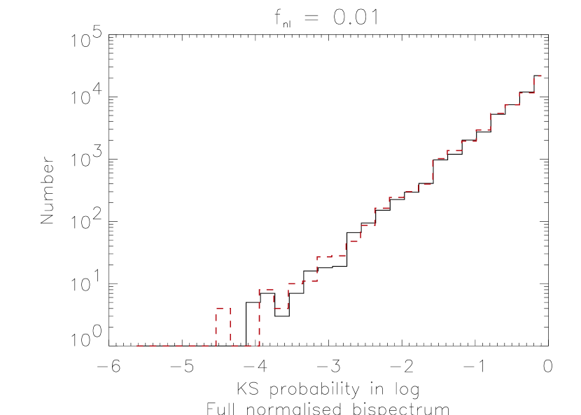
If we now move back from a single test to the estimators as a whole, we are confronted with a new problem which is most noticeable in the case of the bispectrum, for example. There, we perform of the order of $n_{t}\simeq 10^{5}$ tests. Hence, we expect to find some tests (although very few) where even the comparison of two Gaussian ensembles results in a very low probability of order $1/n_{t}$. This is illustrated e.g. by figure 5 where the uniform distribution of the Gaussian probabilities is also clearly visible. Only a deviation from this behaviour signals a violation of the Gaussian hypothesis. As a corollary, if a single test (a single scale) has a probability $P_{KS}\ll 1/n_{t}$, that test alone ensures with near-certainty that the process which created the map is not Gaussian. To avoid any confusion with these small Gaussian probabilities, we state in general both the results of the KS test of non-Gaussian versus Gaussian reference maps as well as the Gaussian counterparts versus Gaussian reference results.

Given the large ensemble of $P_{KS}$ values for the bi- and trispectrum, and knowing their distribution in the Gaussian case (either taking the theoretical uniform distribution or, which is more appropriate, directly the measured values), it is tempting to go one step further and to apply the KS test a second time. This meta-statistics then returns one global meta-probability for the detection of a non-Gaussian signature by a given method, but neglects many aspects such as correlations between the tests which make up that method. In the case of the bi- and trispectrum, the meta-statistics discards the information on the frequency location of the tests and thus weakens the power of the Fourier analysis. In addition, the meta-statistics might also degrade our ability to detect the non-Gaussian signatures due to the known limitations of the KS test. Even if, as an example, a few locations have very small probabilities $P_{KS}\ll 1/n_{t}$, the global meta-probability may be acceptable if those points are not numerous enough. Of course these highly significant values alone would suffice to reject the Gaussian hypothesis.

It is worth noting that the choice of the number of test (non-Gaussian) and reference maps for the first KS test has an important impact on the meta-statistics. If the number of maps in the two sets have not enough different prime factors (e.g. 50 and 100), then heavy aliasing can occur since the KS test is only sensitive to the difference in the values of the cumulative distribution functions. In this case, only very few distinct differences (and hence KS probabilities) exist, leading to a non-continuous distribution of the KS probabilities. As a consequence, the second KS test gives a spuriously low global meta-probability indicating that the signals are statistically quite different, even when comparing Gaussian versus Gaussian maps. To avoid this, we use 50 test maps and 99 reference maps, which largely eliminates the problem.

For the wavelet based estimators, we could also perform meta-statistics. We would in this case have to create a distribution of KS probabilities for each decomposition scale by comparing several sets (Gaussian versus Gaussian and non-Gaussian versus Gaussian), and then apply the KS test a second time. We refrain from applying this method here.

The KS test tends to be more sensitive around the median value of the cumulative distribution function and less sensitive to differences at the extreme ends of the distribution. It is therefore a good test to measure shifts but not so good in finding spreads which might affect the tails of the distribution. A way of accounting for these differences at the tails is to replace the KS distance $d$ by a stabilised or weighted statistics, for example the Andersen-Darling (AD) test or the Kuiper test. In the former test, no probability is computed. This property makes it vital for the estimation of the non-Gaussian detection level that we actually compare on the one hand Gaussian counterparts and the Gaussian reference set, to on the other hand non-Gaussian data set and the reference set. We have checked that both the AD and the Kuiper tests give results that are in quite agreement with the KS test. In the following, we concentrate onto the KS test, and we present the results for each statistical estimator in terms of the probability that two distributions are identical.

4.2 Results from the cumulative probability function

As mentioned before, our baseline is given by a simple comparison between the estimated CPF of the non-Gaussian data sets and the corresponding reference set. We use the KS test for this comparison, since it provides us directly with an estimate of the probability. We do not collect all pixels of all test maps, but use only the pixels of one map at a time and find therefore a distribution of values. Table 1 gives the averaged results obtained in this way, compared to the results from the Gaussian counterpart set. The maps used for this purpose were deconvolved with the average power spectrum extracted from the comparison set.

In all cases, the non-Gaussian signature is clearly detected (with the $f_{NL}=0.01$ $\chi^{2}$ type maps being the least non-Gaussian by far), while the Gaussian counterpart maps are consistent with the Gaussian hypothesis. As the point source maps and the $\chi^{2}$ maps use the same Gaussian reference and counterpart maps, they also share the same Gaussian probability $P_{G}$. That value might be slightly higher than expected due to the deconvolution which has to use an estimated power spectrum (the true one being unknown in practice). But in the worst case, we expect this measure to lead to a weaker detection of non-Gaussianity. If we do not deconvolve the maps, we find, $P_{G}=10^{-3}$ for the point source Gaussian reference set versus the Gaussian counterpart set, and the filament case is much worse.

	Filaments	Point sources	$\chi^{2}$ maps
$P_{KS}$	$0$	$0$	$4.7\cdot 10^{-4}$
$P_{G}$	$0.73$	$0.72$	$0.72$

Table 1: Test for non-Gaussianity using the CPF for all (whitened) maps. The first line is the average KS probability for the real, non-Gaussian maps, the second line the average probability for the Gaussian counterpart set. The $\chi^{2}$ type maps have a non-linear coupling factor $f_{NL}=0.01$.

Additionally, we can quantify the sensitivity of this test to the non-Gaussian signatures present in the $\chi^{2}$ maps. To this end, we form a likelihood estimator ${\cal L}[f_{NL}]$, and find the best-fit parameter $f_{NL}$ by minimising ${\cal L}$. The variation of the recovered $f_{NL}$ for a set of Gaussian maps gives an indication of the sensitivity of the approach. A priori, we could use directly the KS probability as given above for the likelihood function. But, as demonstrated in Santos et al. (2002), it is simpler to use a $\chi^{2}$ fitting procedure to a signal which can be analytically predicted and in which $f_{NL}$ enters linearly. In this case, we can calculate the best-fit value in a very straightforward way.

The probably simplest signals which can be extracted from the CPF are its moments. As the average vanishes, and as all even moments show only a leading order non-Gaussianity proportional to $f_{NL}^{2}\ll 1$, it is best to use the skewness. To first order in $f_{NL}$, we find $<T^{3}>=6f_{NL}\sigma^{4}$, where the standard deviation $\sigma$ is the one of the original Gaussian map. The one recovered from a non-Gaussian $\chi^{2}$ type map differs by a term of order $f_{NL}^{2}$ which can be neglected. The likelihood is then given by

$$\chi^{2}[f_{NL}]=\sum_{\bf x}\frac{\left(T({\bf x})^{3}-f_{NL}6\sigma^{4}\right)^{2}}{15\sigma^{6}}.$$ (28)

Since it is again important to use a whitened map we will assume that $\sigma=1$. We set $\partial\chi^{2}/\partial f_{NL}=0$ and find

$$f_{NL}=\frac{1}{6N^{2}}\sum_{\bf x}T({\bf x})^{3}.$$ (29)

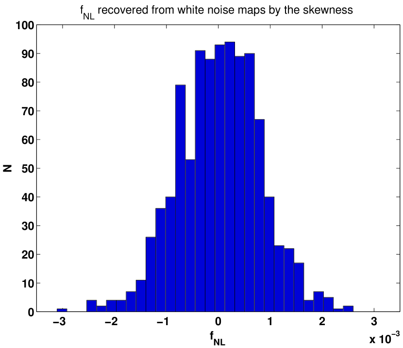
Figure 4 shows the recovered $f_{NL}$ from 1000 maps with Gaussian white noise. Their variance is $\sigma=8.\,10^{-4}$ and we find for the 50 maps with $f_{NL}=0.01$ that $f_{NL}=0.0098\pm 0.0007$.

There is a caveat: In order to extract that value, we needed to know the exact kind of non-Gaussian signal we are dealing with. However, it is valid to use the present procedure to set limits on the parameter in question if no non-Gaussian signal is detected.

Figure 4: The values of $f_{NL}$ recovered from the skewness of 1000 maps which contain Gaussian white noise. The variance is $\Delta f_{NL}=8.\,10^{-4}$.

4.3 Results from the wavelet decomposition

In order to find the non-Gaussian signatures present in the studied signals, we compute the skewness and excess kurtosis of the wavelet coefficients at each decomposition scale and in each sub-band, i.e for the three types of details (horizontal, vertical and diagonal). We compute these quantities for both the Gaussian and non-Gaussian maps and we compare the obtained distributions of skewness and excess kurtosis for the Gaussian and non-Gaussian processes using the KS test. This comparison allows us to get, for each scale and orientation, the probability that the non-Gaussian process and the Gaussian realisations with the same power spectra have the same distribution.

All the obtained probabilities for the skewness and excess kurtosis are given in the tables 2, 3 and 4. In these tables and for each type of details, the first set of 2 lines represents $P_{KS}$ for the skewness. The first line is for non-Gaussian versus reference set comparison, and the second line is for the Gaussian counterpart versus reference set (G vs G). The second set of 2 lines represents the $P_{KS}$ for the excess kurtosis. Again, the first line is for non-Gaussian versus reference set comparison, and the second for the Gaussian counterpart versus reference set.
The probabilities of the order of, or lower than, $10^{-3}$ indicating a non-Gaussian detection at a level $>99.9\%$ are all in shaded boxes. The probabilities obtained from the comparison between the Gaussian counterparts and the reference Gaussian realisations (G vs G) allow us to estimate any possible non-significant detection of non-Gaussian signature, or statistical fluctuation in the Gaussian sets.

4.3.1 Third moment of the wavelet coefficients: Skewness

Confirming the CPF results for which there was a clear detection of non-Gaussian signatures in the set of $\chi^{2}$ maps with a coupling factor $f_{\mathrm{NL}}=0.1$, the non-Gaussian signatures are very easily detected in the wavelet space. We therefore focus on the $\chi^{2}$ maps with a coupling factor $f_{\mathrm{NL}}=0.01$. We summarise the KS probabilities derived from the comparison of the distribution of skewnesses in Table 2, first two lines of each type of details.

	Scale 1	Scale 2	Scale 3	Scale 4	Scale 5	Scale 6
Vertical	2.08$\,10^{-18}$	0.226	0.488	0.828	0.158	0.368
G vs G	0.411	0.450	0.160	0.160	0.791	0.036
	0.488	0.426	0.367	0.426	0.426	0.189
G vs G	0.332	0.791	0.068	0.940	0.411	0.332
Horizontal	1.97$\,10^{-17}$	0.002	0.828	0.555	0.695	0.625
G vs G	0.876	0.207	0.940	0.876	0.940	0.332
	0.315	0.0450	0.625	0.764	0.426	0.226
G vs G	0.264	0.596	0.411	0.940	0.596	0.791
Diagonal	0.001	0.157	0.828	0.368	0.315	0.315
G vs G	0.791	0.596	0.940	0.695	0.049	0.791
	0.828	0.695	0.930	0.828	0.764	0.963
G vs G	0.265	0.265	0.876	0.791	0.499	0.596

Table 2: For the $\chi^{2}$ maps with $f_{\mathrm{N}L}=0.01$: The KS probability (for two signals to have identical distributions) for each of the details at all decomposition scales. For each detail, the first two lines are for the skewness of the wavelet coefficients, and the second two lines represent the excess kurtosis. For each pair, the first line stands for the comparison between the 50 non-Gaussian and 99 reference Gaussian maps, and the second line for the comparison between the 50 Gaussian counterparts and 99 reference Gaussian maps (G vs G). All probabilities lower than $10^{-3}$ are in shaded boxes.

For these $\chi^{2}$ maps, the departure from the Gaussian hypothesis is only detected at the first wavelet decomposition scale (i.e 3 arc minutes). Both the vertical and horizontal details appear very sensitive to the non-Gaussian features present in the maps. The non-Gaussian signatures are also detected in the diagonal details, at the first scale, but with a much lower confidence level. From the KS probabilities obtained from the comparison Gaussian counterparts versus Gaussian reference maps (second line of the first set in each detail), it is obvious that the detection of the non-Gaussian signatures are highly significant. It is however worth noting that we detect some fortuitous non-Gaussian signatures, at 93 to 96% confidence levels, due to statistical fluctuations when we compare the Gaussian maps with the reference Gaussian set.

In the case of the filaments (Table 3, first two lines of each type of detail), the KS test for the skewness distribution of the non-Gaussian against the Gaussian reference set shows that the non-Gaussian features are detected at all scales (with less confidence at scale 6). The detection takes place for the three types of details. We note that the probability for the non-Gaussian signal to be compatible with a Gaussian process increases for the highest decomposition levels, i.e. the largest angular scales, as it is expected from our studied signal in which the filamentary structures have not increasingly large sizes.

As for the point sources (Table 4, first two lines of each type of details), the non-Gaussian signatures do not show up very significantly (whatever decomposition scale and details). The obtained probabilities remain always larger than $\simeq 0.002$ suggesting a non-Gaussian detection at a $\simeq 99.8\%$ confidence level at best.

For the filamentary structures as well as for the point sources, the comparison between Gaussian counterparts and Gaussian reference (G vs G) set shows that we are very much compatible with identity test (processes having the same distribution). The obtained KS probabilities show the high level of significance of the non-Gaussian detection.

	Scale 1	Scale 2	Scale 3	Scale 4	Scale 5	Scale 6
Vertical	1.27$\,10^{-7}$	6.54$\,10^{-15}$	1.77$\,10^{-11}$	1.65$\,10^{-8}$	5.25$\,10^{-8}$	0.047
G vs G	0.743	0.911	0.486	0.879	0.320	0.239
	3.3$\,10^{-20}$	3.3$\,10^{-20}$	3.3$\,10^{-20}$	3.3$\,10^{-20}$	1.01$\,10^{-16}$	1.09$\,10^{-6}$
G vs G	0.379	0.574	0.471	0.996	0.682	0.879
Horizontal	1.77$\,10^{-11}$	1.43$\,10^{-12}$	1.9$\,10^{-9}$	1.77$\,10^{-11}$	9.23$\,10^{-8}$	0.001
G vs G	0.651	0.788	0.976	0.391	0.515	0.998
	3.3$\,10^{-20}$	3.3$\,10^{-20}$	3.3$\,10^{-20}$	3.3$\,10^{-20}$	1.22$\,10^{-18}$	7.68$\,10^{-9}$
G vs G	0.773	0.066	0.829	0.258	0.088	0.559
Diagonal	5.13$\,10^{-7}$	2.85$\,10^{-5}$	1.65$\,10^{-8}$	0.0004	0.010	0.008
G vs G	0.682	0.142	0.040	0.651	0.842	0.682
	3.3$\,10^{-20}$	3.3$\,10^{-20}$	3.3$\,10^{-20}$	3.3$\,10^{-20}$	3.7$\,10^{-16}$	5.69$\,10^{-8}$
G vs G	0.636	0.529	0.758	0.816	0.379	0.040

Table 3: For the filaments: The KS probability (for two signals to have identical distributions) for each of the details at all decomposition scales. For each detail, the first two lines are for the skewness of the wavelet coefficients, and the second two lines represent the excess kurtosis. For each pair, the first line stands for the comparison between the 28 non-Gaussian and 99 reference Gaussian maps, and the second line for the comparison between the 28 Gaussian counterparts and 99 reference Gaussian maps (G vs G). All probabilities lower than $10^{-3}$ are in shaded boxes.

4.3.2 Fourth moment of the wavelet coefficients: Excess kurtosis

We now turn to the fourth moment in the wavelet space, i.e. the excess kurtosis of the wavelet coefficients. The results are given by the second sets of two lines in Tables 2, 3 and 4. Again the first line is for the KS probability obtained from the comparison of non-Gaussian maps with Gaussian reference set, and the second line stands for the comparison of Gaussian counterparts versus reference set (G vs G).

In the case of the $\chi^{2}$ maps with $f_{\mathrm{N}L}=0.01$, the fourth moment do not, as expected, exhibit any departure from the Gaussian hypothesis. This is demonstrated by the large values of the KS probabilities (Table 2, second sets of lines).

The point sources (Table 4, first line of the second set of lines for each detail), exhibit very highly non-Gaussian signatures as shown by the small KS probabilities (always smaller than $\simeq 10^{-5}$). Furthermore, the non-Gaussian signatures are present at all decomposition scales and for all the details. We compare the obtained probabilities with those derived from the comparison of Gaussian counterparts with Gaussian reference set. We note the high level of significance of the non-Gaussian detections.

The same kind of results (detection of non-Gaussian features at all scales with all details) are obtained for the filaments (Table 3, second sets of lines) for which the probability that the non-Gaussian maps are statistically equivalent to the Gaussian reference maps is always smaller than $10^{-6}$. We have again computed the KS probabilities for the excess kurtosis of the wavelet coefficients from the comparison of Gaussian maps. This comparison shows that the two sets of maps are statistically the same which conversely reinforces the level of significance of the non-Gaussian detection in the filament maps.

	Scale 1	Scale 2	Scale 3	Scale 4	Scale 5	Scale 6
Vertical	0.012	0.791	0.002	0.008	0.411	0.791
G vs G	0.791	0.265	0.122	0.332	0.791	0.160
	3.47$\,10^{-30}$	3.47$\,10^{-30}$	3.47$\,10^{-30}$	6.12$\,10^{-24}$	0.001	0.411
G vs G	0.265	0.876	0.207	0.999	0.499	0.160
Horizontal	0.122	0.695	0.265	0.006	0.265	0.791
G vs G	0.596	0.411	0.876	0.411	0.499	0.596
	3.47$\,10^{-30}$	3.47$\,10^{-30}$	3.47$\,10^{-30}$	2.3$\,10^{-22}$	1.42$\,10^{-6}$	0.068
G vs G	0.411	0.499	0.122	0.791	0.695	0.596
Diagonal	0.012	0.160	0.596	0.596	0.876	0.332
G vs G	0.695	0.996	0.940	0.876	0.207	0.160
	3.47$\,10^{-30}$	3.47$\,10^{-30}$	1.09$\,10^{-26}$	9.87$\,10^{-16}$	1.02$\,10^{-7}$	0.0004
G vs G	0.092	0.160	0.876	0.791	0.596	0.499

Table 4: For the point sources: The KS probability (for two signals to have identical distributions) for each of the details at all decomposition scales. For each detail, the first two lines are for the skewness of the wavelet coefficients, and the second two lines represent the excess kurtosis. For each pair, the first line stands for the comparison between the 50 non-Gaussian and 99 reference Gaussian maps, and the second line for the comparison between the 50 Gaussian counterparts and 99 reference Gaussian maps (G vs G). All probabilities lower than $10^{-3}$ are in shaded boxes.

4.4 Results from the bispectrum

Similarly to the wavelet coefficients, we compare for each triplet $(\ell_{1},\ell_{2},\ell_{3})$ the distributions of the (normalised) bispectrum values, as described in section 3.3, for the non-Gaussian realisations and for the Gaussian reference set. Hence, we associate to each triplet $(\ell_{1},\ell_{2},\ell_{3})$ two ensembles of bispectrum coefficients – on the one hand 50 or 28 values for the non-Gaussian maps, and on the the other hand 99 values for the Gaussian reference set. Using the KS test, we therefore end up for each triplet with a probability that the signals are drawn from the same process, i.e. that the non-Gaussian maps are compatible with the Gaussian reference set.

For the full bispectrum, we limit ourselves to a bandwidth of four pixels, but probe additionally the diagonal elements with a bandwidth of two pixels. We have tested that using the higher resolution for the full bispectrum does not lead to a better detection of the non-Gaussian signal for the $\chi^{2}$ type maps, and does not improve the variance of the recovered value of $f_{NL}$ (see the following subsection).

For the sake of a clearer visual representation of the results, we choose to show the KS probabilities as a function of the surface and the smallest angle defined by the triplet, rather than as a function of the triplet itself. Note that we are speaking of surfaces and angles in Fourier space.

4.4.1 $\chi^{2}$ maps

We first focus on the case of the non-Gaussian $\chi^{2}$ maps with a coupling factor of $f_{\mathrm{NL}}=0.01$. We find, for the full bispectrum, that the probabilities for the non-Gaussian signal to be compatible with its Gaussian reference set are as low as a few times $10^{-6}$. However as mentioned in section 4.1 (see also Fig. 5), the comparison of the 50 Gaussian counterpart realisations to the reference set of 99 Gaussian maps gives KS probabilities of the same order, and it is hard to say whether there is a detection of non-Gaussianity or not. If we apply the KS test a second time, now to the two resulting distributions of probabilities, the global meta-probability obtained is $4.1\,10^{-4}$. The bispectrum therefore does indeed detect this type of non-Gaussian signatures.

Figure 5: For the $\chi^{2}$ maps with non-linear coupling factor $f_{NL}=0.01$: Distribution of the KS probabilities obtained by i) comparing the full normalised bispectrum estimator of the non-Gaussian maps to the Gaussian reference set (dashed line), and ii) comparing the same quantity for the Gaussian counterparts to the Gaussian reference set (solid line). In the second case, the probabilities are distributed uniformly. The slope is due to the log-log representation we have chosen.

As the bispectrum shares many properties with the skewness, we would expect it to be rather good at detecting $\chi^{2}$ type non-Gaussianity. Given the way in which we construct our test maps, the theoretical signal is

$$B^{(th)}_{\ell_{1}\ell_{2}\ell_{3}}=6f_{NL}\sqrt{C_{\ell_{1}}C_{\ell_{2}}C_{\ell_{3}}}.$$ (30)

We can eliminate any dependence on the power spectrum by using the $C_{\ell}$- normalised estimator. The $\chi^{2}$ likelihood function is then (denoting a triplet $(\ell_{1},\ell_{2},\ell_{3})$ by $\alpha$) very similar to the one for the CPF, eq. (28),

$$\chi^{2}[f_{NL}]=\sum_{\alpha}\frac{\left(B_{\alpha}^{(obs)}-6f_{NL}\right)^{2}}{\sigma_{\alpha}^{2}}$$ (31)

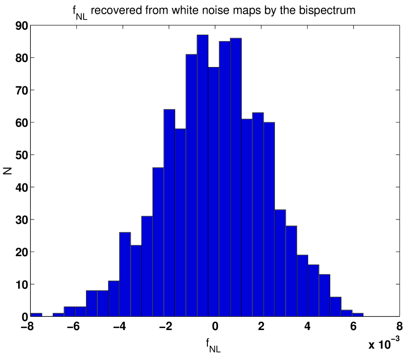
and since the dependence of $\partial\chi^{2}/\partial f_{NL}=0$ on $f_{NL}$ is linear we can again solve for it analytically. By using this method, we recover $f_{NL}=0.010\pm 0.002$ and find that the 1000 Gaussian white noise maps have a variance of $0.0023$ (see Fig. 6). As mentioned earlier, using a bandwidth of two instead of four does not improve the sensitivity. One should not forget, though, that the Fourier space methods are better adapted to spherical spaces, where the scale decomposition is automatic and does not need to be imposed by placing rings on a rectangular grid. Furthermore, the skewness is always just a number, while a realistic model of primary non-Gaussian signatures (taking into account the radiation transfer function) introduces a non-trivial shape and even sign changes into eq. (30), see e.g. Santos et al. (2002). In the presence of several different kinds of non-Gaussian signatures, the bispectrum should be better at discriminating between them in that case, and also using a lower bandwidth may become useful.

Figure 6: The values of $f_{NL}$ recovered from the bispectrum of 1000 maps which contain Gaussian white noise. The variance is $\Delta f_{NL}=2.\,10^{-3}$.

4.4.2 Point sources

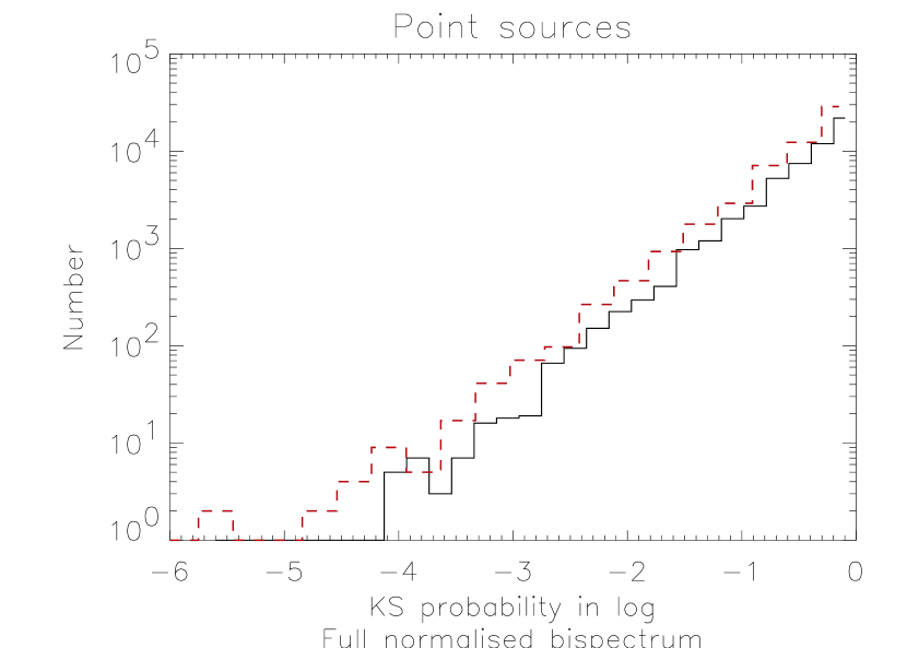
In the case of the non-Gaussian maps made of a distribution of point sources, the KS test gives again probabilities down to $10^{-6}$ for the full bispectrum, apart from a single point with much lower probability ($P_{KS}\simeq 10^{-9}$). We concentrate onto the full bispectrum tests and we need to compare the obtained KS probabilities with the ones derived from the comparison of 50 Gaussian counterparts versus the reference set. The figure 7 displays the distribution of KS probabilities. We note in particular that the non-Gaussian signal exhibits an excess of low KS probabilities as compared with the probabilities from Gaussian vs reference set. This difference between the two distributions is confirmed by the meta-statistics which gives a probability of $8.6\,10^{-4}$.

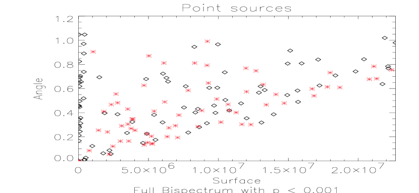
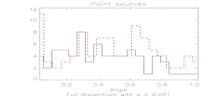
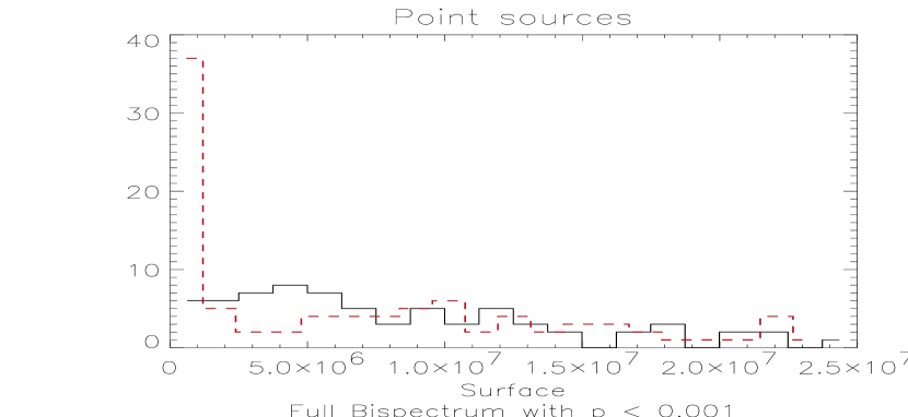
Let us now concentrate onto the KS probabilities that are lower than $10^{-3}$. We display in the surface-angle plane the results of the non-Gaussian vs reference set comparison (Fig. 8, diamonds) and Gaussian counterparts vs reference set (Fig. 8, asterisks). We notice that for small surfaces (in $\ell$ space, i.e. Fourier space) the majority of points are associated with the non-Gaussian maps. There are no detections associated with the Gaussian vs reference set comparison. This is even more obvious when we plot the distribution of surfaces for KS probabilities $<10^{-3}$ (Fig. 8 lower panel, histogram of surfaces). The first bin is indeed dominated by the detections from the non-Gaussian versus reference set comparison. The small surfaces in Fourier space are associated with large surfaces in real space ($x\propto 1/\ell$). The result we obtain indicates that we are actually detecting the non-Gaussian signatures associated with the higher amplitude spots in the maps (Fig. 1, upper left panel) that are also spatially more extended and lying on a crowded background of smaller sources. The histogram of angles (Fig. 8, middle panel) in turn does not show any highly significant difference between the non-Gaussian versus reference and Gaussian counterpart versus reference.

Figure 7: For the point sources: Distribution of the KS probabilities for the full bispectrum. The dashed line represents the results from the comparison of non-Gaussian maps to Gaussian reference set. The solid line is for the comparison Gaussian counterparts versus reference set.

Figure 8: For the point sources: The KS probabilities lower than $10^{-3}$. In the surface-angle plane (upper panel) defined by the triplets, the asterisks are for the comparison Gaussian counterparts versus reference set, and the diamonds for the comparison non-Gaussian maps versus reference set. The middle panel shows the distribution of angles for the above selected KS probabilities. The lower panel shows the distribution of surfaces for the same selection. The dashed line is for non-Gaussian versus reference set, and the solid line for Gaussian versus reference set.

4.4.3 Filaments

Our last non-Gaussian data set is constituted of the 28 modified IRAS maps representing the filamentary structures. This process is by far the most non-Gaussian. The KS test between the distribution of bispectrum values for the 28 non-Gaussian maps and 99 Gaussian reference maps goes down to $10^{-20}$ for the full bispectrum. Similarly to the other processes, we also compare 28 Gaussian realisations to the reference set in order to estimate the significance of the detections. In the case of the filaments, there is no doubt that the non-Gaussian signatures are detected. This is exhibited (Fig. 9) by the difference in the distribution

Figure 9: For the filaments: Distribution of the KS probabilities for the full bispectrum. The dashed line represents the results by comparing the non-Gaussian maps to the Gaussian reference set. The solid line is for the comparison Gaussian counterparts versus reference set.

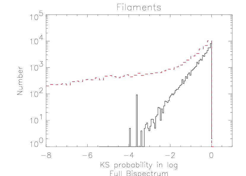
of KS probabilities obtained when comparing the non-Gaussian maps to the Gaussian reference set (dashed line), and the probabilities resulting from the comparison of 28 Gaussian realisations versus the Gaussian reference set (solid line). Unsurprisingly, the meta-statistics returns a probability of 0 confirming the very high significance of the non-Gaussian detection.

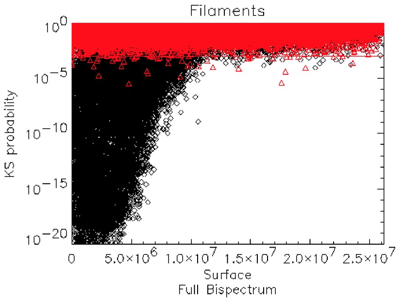
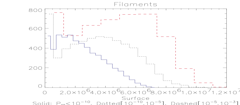
In Fig. 10, we display both the Gaussian vs Gaussian (gray triangles), and non-Gaussian vs Gaussian (black diamonds) points. We note that most of the probabilities in the Gaussian vs Gaussian case lie above the $10^{-3}$ limit (horizontal solid line). The non-Gaussian character is very strongly localised in the triplets with small surfaces. The distribution as a function of angle is much more uniform.

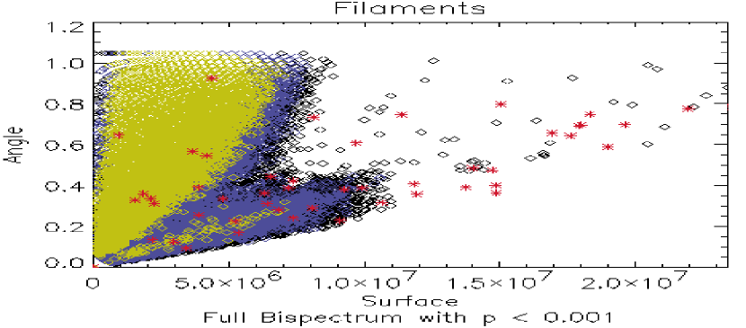
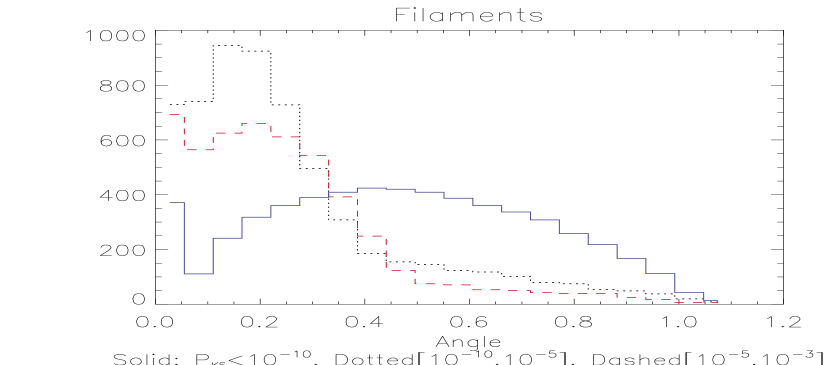
If we study the KS probability as a function of both angle and surface (see figure 11), we find that the non-Gaussian signatures are mainly localised in two distinct “plumes”. The first contains triplets with angles basically no larger than 0.4 radian and surfaces that are as large as $10^{7}$, while the second, larger plume, covers all angles but only triplets with a slightly smaller surface. The two histograms, in Fig. 11, show the number of triplets within a range of KS probability as a function of either surface or smallest angle. They show that the very lowest probabilities (solid line) are associated with the second, larger plume. They are distributed over a wide range of angles, but have all a small surface. The intermediate probabilities are concentrated in triplets with small angles but a wider range of surfaces. These figures show that the bispectrum allows very detailed analysis of the non-Gaussianity present in a data set, if it is detected at a sufficiently high level.

Figure 10: The filament maps: KS probabilities from the comparison of the full bispectrum as a function of the surface defined by the triplet. Black diamonds represent the results obtained from the comparison non-Gaussian maps versus Gaussian reference set. Gray triangles represent the results obtained from the comparison Gaussian counterparts versus reference set. The solid horizontal line indicates the limit for $P_{KS}=10^{-3}$.

Figure 11: For the full bispectrum of the filaments: Distribution of KS probabilities in the surface-angle plane defined by the triplets (upper panel). Diamonds are for the comparison non-Gaussian maps versus Gaussian reference set. Black diamonds are for the KS probabilities comprised between $10^{-5}$ and $10^{-3}$, gray diamonds represent $10^{-10}<P_{KS}<10^{-5}$, and light gray diamonds stand for $P_{KS}<10^{-10}$. The asterisks are for the comparison Gaussian counterparts versus reference set. The middle panel shows the distribution of angles for the above selected KS probabilities. The lower panel shows the distribution of surfaces for the same selection. Dashed lines are for $10^{-5}<P_{KS}<10^{-3}$, dotted lines represent $10^{-10}<P_{KS}<10^{-5}$, and solid lines stand for $P_{KS}<10^{-10}$.

4.5 Results from the trispectrum

Following the same approach as for the bispectrum and as explained in detail in section 4.1, we compare for each pair $(\ell,a)$ the distribution of the trispectrum values (defined as in section 3.3) for the non-Gaussian set and for its Gaussian reference set. We compare the sensitivity of the two estimators $T^{(0)}$ and $T^{(+)}$ (respectively diagonal and near-diagonal trispectra) in terms of non-Gaussian detection on the point source maps since the signal is non-Gaussian but not as extreme as in the filaments.

As a significance discriminator, we use the equivalent results from the comparison between the set of Gaussian counterpart maps and the Gaussian reference set. We checked that the normalisation of the trispectrum to the power spectrum does not affect the resulting KS probabilities significantly.

4.5.1 $\chi^{2}$ maps

For the $f_{\mathrm{N}L}=0.01$ $\chi^{2}$ maps and Gaussian maps, the smallest KS probabilities are a few times $10^{-5}$, see Fig. 12. The meta-statistics confirms that we do not see any significant deviation from the Gaussian hypothesis: The orthonormalised $T^{(+)}$ estimator leads to a meta–$P_{KS}=0.13$ for a non-linear coupling constant of $0.01$.

It is not surprising that the trispectrum does not detect any non-Gaussian signature. Just as for the excess kurtosis of the pixel distribution in real space (see section 4.2), the lowest order contribution to the trispectrum is proportional to $f_{NL}^{2}$. This makes it naturally much less suited to find this kind of non-Gaussian signals. This fact can however be used as a counter-check, since if we believe to have detected a $\chi^{2}$ type signal in the bispectrum, we should not find it when applying the trispectrum to perfectly clean data.

Figure 12: For the $\chi^{2}$ maps with non-linear coupling factor $f_{NL}=0.01$: Distribution of the KS probabilities obtained by i) comparing the trispectrum estimators of the non-Gaussian maps to those of the Gaussian reference set (dashed line), and ii) comparing the trispectrum estimators of the Gaussian counterparts to those of the Gaussian reference set (solid line).

4.5.2 Point sources

The histogram of probability values in figure 13 (upper panel) does not show any extreme differences for $T^{(+)}$ between the Gaussian vs Gaussian and the non-Gaussian vs Gaussian comparisons, with only one value at $(\ell,a)\simeq(300,0)$ having a particularly low probability of $10^{-8}$. The global

Figure 13: For the point sources: Distribution of the KS probabilities obtained by i) comparing the trispectrum estimators of the non-Gaussian maps to those of the Gaussian reference set (dashed line), and ii) comparing the trispectrum estimators of the Gaussian counterparts to those of the Gaussian reference set (solid line). The upper panel is for the near-diagonal trispectrum ($T^{(+)}$) and the lower panel for the diagonal trispectrum estimator ($T^{(0)}$).

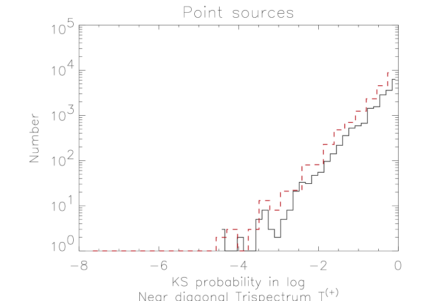
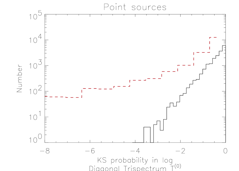
probability for being Gaussian is $8.8\,10^{-4}$. This changes dramatically if we look at $T^{(0)}$ (Fig. 13, lower panel). The diagonal estimator detects a very clear non-Gaussian signal, and the meta-statistics returns a probability of $0$. It is quite surprising that the two estimators show such a huge difference, although they are indeed completely independent, since $T^{(+)}$ does not have any Gaussian contribution, as opposed to $T^{(0)}$.

Figure 14: For the trispectrum of the point sources: Distribution, in ($\ell$,$a$) space, of the KS probabilities lower than $10^{-3}$. Asterisks are for the comparison between Gaussian counterparts and Gaussian reference set. Diamonds stand for the non-Gaussian versus Gaussian reference set comparison. The upper panel is for the near-diagonal trispectrum. Most diamonds are found at very small $a$ in this case. The lower panel is for the diagonal trispectrum estimator.

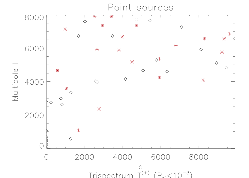
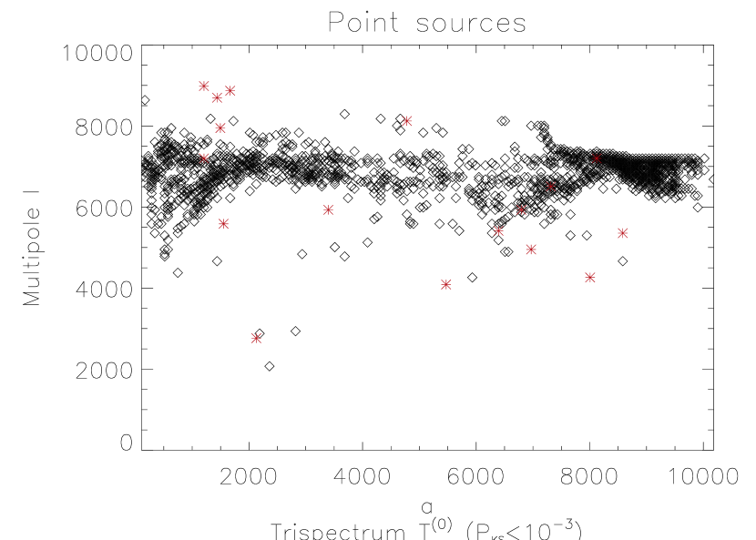
Looking at the distribution of the low-probability points in $(\ell,a)$ space (Fig. 14 upper and lower panels), we find that $T^{(0)}$ is localised around $\ell\approx 7000$ and seems to prefer either very small or very large values of $a$, corresponding to oblong configurations. The weak signal of $T^{(+)}$ seems to be mainly due to points with low $\ell$ and very small $a$ (diamonds in Fig. 14 upper panel).

4.5.3 Filaments

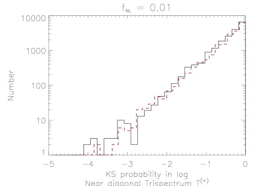
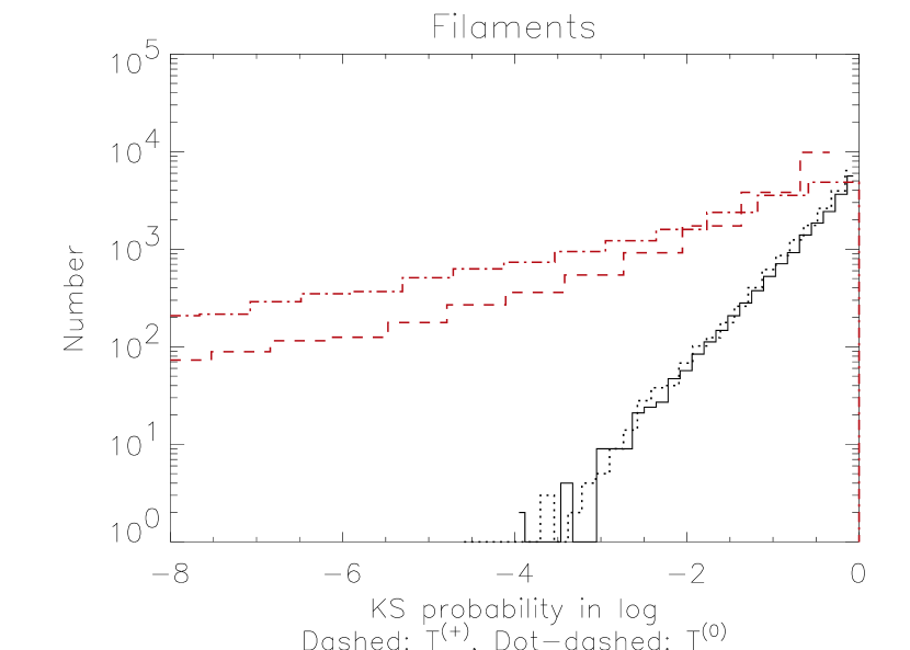
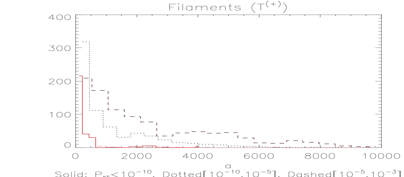
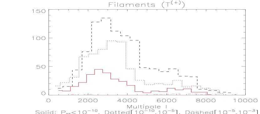
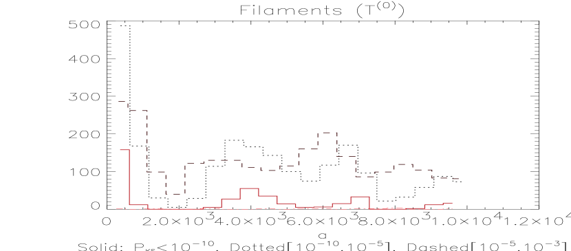
For the case of the non-Gaussian filament maps, the KS test gives probabilities that the non-Gaussian signal is issued from the same process as the Gaussian reference set as low as a few $10^{-20}$. Figure 15 shows the difference in the distributions of the KS probabilities for diagonal and near-diagonal trispectrum. Furthermore, the meta-probability obtained by applying the KS test on these probability distributions returns 0. In this case and similarly to the bispectrum, the non-Gaussian signatures are consequently undoubtedly detected. However, again the diagonal estimator seems more sensitive than the near-diagonal trispectrum. As shown in Fig. 15, there are many more (twice as many) low probabilities (high confidence detection) in the diagonal case than in the near-diagonal.

Figure 15: For the trispectrum of the filaments: Distribution of KS probabilities. The solid line is for the comparison of Gaussian counterparts vs Gaussian reference set for the near-diagonal estimator ($T^{(+)}$). The dashed line is for the comparison of the non-Gaussian maps to reference set for the near-diagonal trispectrum. The dotted line is for the comparison of Gaussian counterparts vs reference set for the diagonal trispectrum ($T^{(0)}$). The dot-dashed line is for the non-Gaussian maps vs reference set for the diagonal estimator.

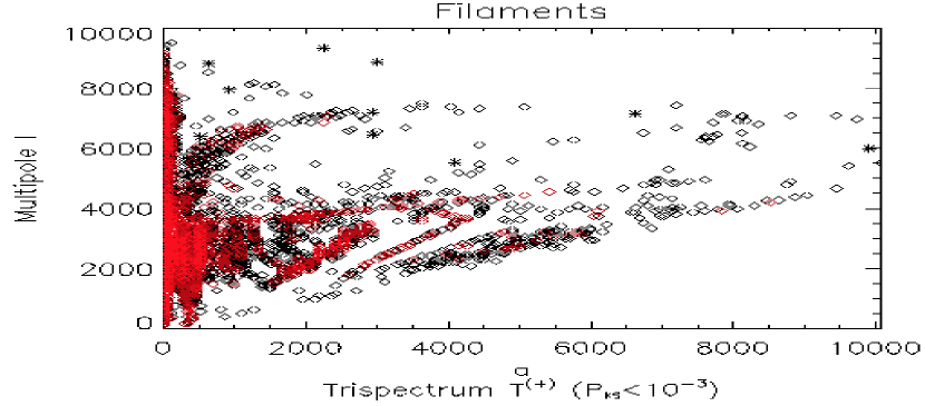
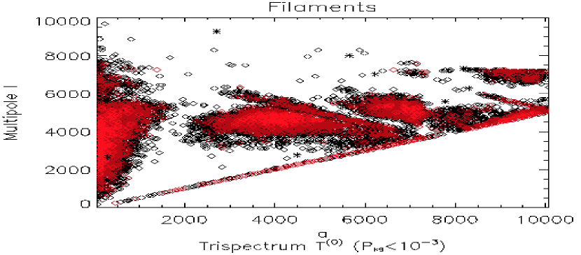
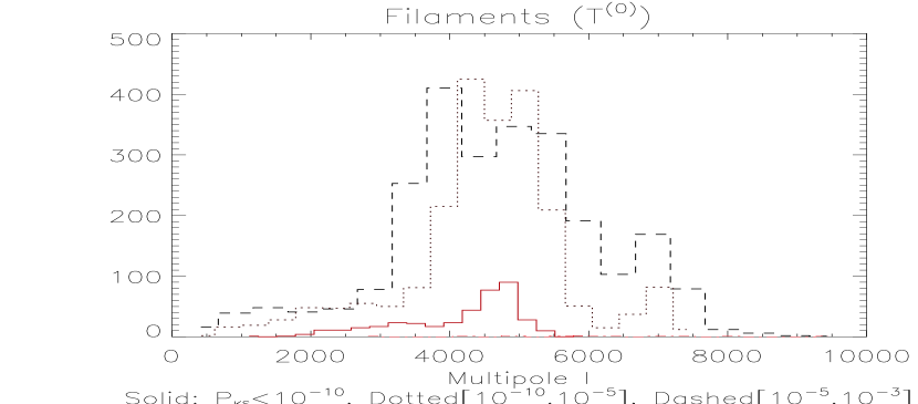
We try to visualise the morphological information contained in the trispectrum coefficients by displaying in $(\ell,a)$ space the KS probabilities (Figs. 16 and 17, upper panels). Those associated with the detection of the non-Gaussian signatures are in diamonds, and those associated with statistical fluctuations in the Gaussian realisations are in asterisks. We plot in figures 16 and 17 the distribution of $a$ and $\ell$ in bins of KS probabilities for the trispectrum ($T^{(+)}$) and ($T^{(0)}$). Both trispectra prefer small values of $a$ (or the diagonal $a\sim 2\ell$ which correspond to similar configurations), which are associated with strongly elongated structures. The diagonal trispectrum exhibits several other low- probability “blobs” at intermediate $a$ values, but the corresponding histogram (the middle panel of Fig. 17) shows that these are somewhat less important. On the $\ell$ axis, $T^{(0)}$ seems non-Gaussian mainly for values between $4000$ and $6000$, while $T^{(+)}$ rather detects a signal around $\ell=2000-4000$. All in all, the two trispectra together show a rich structure with clear concentrations of non-Gaussian signatures, not just random scatter.

Figure 16: For the near-diagonal trispectrum estimator of the filaments: The KS probabilities lower than $10^{-3}$ in the ($\ell$,$a$) space (upper panel). The asterisks are for the comparison Gaussian counterparts versus reference set, and the diamonds for the comparison non-Gaussian maps versus reference set. The middle panel shows the distribution of $a$ for the above selected KS probabilities. The lower panel shows the distribution of $\ell$ for the same selection. Dashed lines are for $10^{-5}<P_{KS}<10^{-3}$, dotted lines represent $10^{-10}<P_{KS}<10^{-5}$, and solid lines stand for $P_{KS}<10^{-10}$.

Figure 17: For the diagonal trispectrum estimator of the filaments: The KS probabilities lower than $10^{-3}$ in the ($\ell$,$a$) space (upper panel). The asterisks are for the comparison Gaussian counterparts versus reference set, and the diamonds for the comparison non-Gaussian maps versus reference set. The middle panel shows the distribution of $a$ for the above selected KS probabilities. The lower panel shows the distribution of $\ell$ for the same selection. Dashed lines are for $10^{-5}<P_{KS}<10^{-3}$, dotted lines represent $10^{-10}<P_{KS}<10^{-5}$, and solid lines stand for $P_{KS}<10^{-10}$.

5 Conclusions

In the present study, we investigate two of the major families of non-Gaussian estimators, namely Fourier-space based methods (the bi- and trispectrum) and wavelet-space based methods (the skewness and excess kurtosis of the wavelet coefficients). They are applied to three quite different data sets chosen to represent a rather complete sample of possible non-Gaussian signatures (namely: point sources, filaments, non-linearly coupled signals). Additionally, the methods were applied to two sets of Gaussian realisations (called reference set and counterpart set) with the same power spectra as the non-Gaussian maps. We then use the Kolmogorov-Smirnov test to quantify the level of detection of the non-Gaussian signatures by comparing the distributions of the estimator values for the non-Gaussian maps versus the Gaussian reference set, and for the Gaussian counterpart set versus the reference set. The first comparison returns directly an estimate of the non-Gaussianity detected by a method, while the second case serves to illustrate the statistical fluctuations within the Gaussian signal itself. Furthermore, we have checked that other statistical tests such as the Kuiper and Anderson-Darling tests give the same results.

We find that the filaments represent a highly non-Gaussian signal. This statistical character is undoubtedly detected by both the Fourier and wavelet based methods in the three and four point estimators. For the point source maps, the non-Gaussian signatures are very significantly detected with the excess kurtosis of the wavelet coefficients and the diagonal estimator of the trispectrum, but less significantly with the bispectrum and very marginally with the skewness of the wavelet coefficients. This is consistent with the moments of the maps, where the non-Gaussianity shows up in the excess kurtosis as well. It is also expected from the physical nature of the signal: The maps contain the same number of negative and positive sources, on average, which suppresses the skewness. The $\chi^{2}$ type maps show just the inverse behaviour, in that it is now the three point tests (skewness of the pixel distribution and of the wavelet coefficients as well as the bispectrum) which detect the non-Gaussian character best. As mentioned earlier this is related to the signal itself which is constructed by adding a positive contribution.

When assessing the relative level of detection, we notice that the wavelet analysis finds the non-Gaussian signatures in the $\chi^{2}$ maps with a non-linear coupling coefficient of 1% at a very high confidence but only at the first decomposition scale (3 arc minute scale), while the bispectrum detection is somewhere between $3$ and $4\sigma$. Wavelets are therefore better at placing constraints on $f_{\rm NL}$, a result which confirms the conclusion of a recent analysis of the COBE-DMR maps with wavelets by Cayon et al. (2002). The point source maps are clearly recognised as non-Gaussian by all methods. Finally we note that the diagonal trispectrum estimator is surprisingly much more sensitive than the nearly diagonal estimator, even though the latter does not contain a Gaussian contribution. This shows that care must be taken if not all components of a given estimator are computed, as the signal may be extremely localised. A forthcoming study will address this question in more detail.

Comparing the methods on a more fundamental level, we find as an additional advantage of the wavelet-based approach that it allows us to associate the non-Gaussian signatures with the features that have caused them in the map, at all the scales where they exist. Wavelet decomposition thus permits to take benefit of any scale-scale correlations that might exist in the non-Gaussian signal. This can be done directly in the wavelet space or by selecting the coefficients and reconstructing the signal with the inverse wavelet transform. These aspects have not been investigated in the present study.

However, the wavelet based estimators are lacking one important property of the Fourier approach. The bi- and trispectrum can be analytically predicted without resorting to Monte Carlo based methods. They can thus be directly related to physical phenomena, which explains their interest for cosmology. Additionally, the bi- and trispectrum allow us to probe a very large number of geometrical configurations for the triplets and quadruplets as compared to the limited number of decomposition scales investigated by the wavelets.

The present comparison can be extended in terms of general strategy proposed to the groups analysing large CMB data sets. If we try to condense it into a few recommendations, we end up with the following steps:

1. Look at the higher order moments in pixel space and the CPF first. The cumulative probability function is very easy and fast to calculate. Nonetheless, it seems to have a similar power as the bi- and trispectrum where just the detection of non-Gaussian signatures is concerned. It therefore provides a quick check if one can expect to find a strong signal with the more sophisticated analysis techniques. We recommend that the maps are deconvolved with their power spectrum before testing the CPF.

2. Apply wavelet based methods second. Wavelets have the highest detection power of the methods presented here, and are only moderately more expensive to apply than the CPF test. If indeed a signal is detected, they can reconstruct its origin in pixel space.

3. Use Fourier methods for a detailed analysis. Together, the bi- and trispectrum furnish a large number of coefficients associated with different geometrical configurations. As the number of theoretical predictions for the bi- and trispectrum from various sources of non-Gaussian signatures is increasing, this allows a precise characterisation of any strong and detected non-Gaussianity in a map, and the use of accurate matched filters to determine its possible origin.

Clearly, combining both wavelet and Fourier based analyses seems the best strategy for studying the non-Gaussian signals. Together, they allow for very significant detections of the non-Gaussian signatures and a large amount of spatial information. In addition, they offer a theoretical basis to relate the physical processes to the measured quantities. Therefore, these methods offer currently the best chances of success when trying to identify the origin of the various sources of non-Gaussian signatures that are expected to contribute to the CMB signal.