A mid-infrared spectroscopic survey of starburst galaxies: excitation and abundances

We present spectroscopy of mid-infrared emission lines in twelve starburst regions, located in eleven starburst galaxies, for which a significant number of lines between 2.38 and 45$\mu m$ were observed with the ISO Short Wavelength Spectrometer, with the intention of providing a reference resource for mid-infrared spectra of starburst galaxies. The observation apertures were centred on actively star forming regions, including those which are inaccessible at optical wavelengths due to high levels of obscuration. We use this data set, which includes fine structure and hydrogen recombination lines, to investigate excitation and to derive gas phase abundances of neon, argon, and sulphur of the starburst galaxies. The derived Ne abundances span approximately an order of magnitude, up to values of $\sim 3$ times solar. The excitation ratios measured from the Ne and Ar lines correlate well with each other (positively) and with abundances (negatively). Both in excitation and abundance, a separation of objects with visible Wolf-Rayet features (high excitation, low abundance) is noted from those without (low excitation, high abundance). For a given abundance, the starbursts are of relatively lower excitation than a comparative sample of H II regions, possibly due to ageing stellar populations. By considering the abundance ratios of S with Ne and Ar we find that, in our higher metallicity systems, S is relatively underabundant by a factor of $\sim 3$. We discuss the origin of this deficit and favour depletion of S onto dust grains as a likely explanation. This weakness of the mid-infrared fine structure lines of sulphur has ramifications for future infrared missions such as SIRTF and Herschel since it indicates that the S lines are less favourable tracers of star formation than is suggested by nebular models which do not consider this effect.

In a related paper (Sturm et al. 2002), we combine our results with spectra of Seyfert galaxies in order to derive diagnostic diagrams which can effectively discriminate between the two types of activity in obscured regions on the basis of excitation derived from detected mid-infrared lines.

1 Introduction

By definition, starburst galaxies are hosts to sites of recent star formation with associated rates that cannot be maintained over a Hubble time, which can be much higher than that determined for the Milky Way. Starburst galaxies are believed to contribute significantly to the population of massive stars in the Universe (Gallego et al. 1995). Within 10Mpc, approximately 25% of high mass star formation is attributed to only four starburst galaxies (Heckman et al. 1998). The reported increase in the star formation density of the Universe for $0.1\la z\la 2$ (e.g. Madau et al. 1996; Madau, Pozzetti, & Dickinson 1998; Barger, Cowie, & Richards 2000) and the high frequency of starbursts with disturbed morphologies or in interacting/merging systems both imply that starbursts are likely to play an important role in galaxy formation and evolution scenarios. By virtue of their proximity, local starbursts can be used as astrophysical laboratories to investigate the processes that may be ongoing at higher redshifts. However, despite intensive observational and theoretical modelling campaigns, the properties of local starbursts are still not fully understood. In particular, their stellar populations and the state of the interstellar medium remain difficult to constrain.

Observable expressions of a starburst depend upon a number of factors, including the stellar initial mass function (IMF), star formation history and the ageing/evolution of the stellar population. Both the evolution of the stellar population and the spectra of individual stars are a function of metallicity, which provides the motivation for studying the effects of metallicity that we consider in this paper. A galaxy’s interstellar medium affects nebular diagnostics and, through obscuration, also direct stellar ones. The widely used local Scalo (1986) IMF may not be reflective of the stellar mass content for starburst galaxies. IMFs modified at either the low or high mass end have been invoked to explain observationally derived properties of starbursts such as dynamical masses, spectral line strengths, continuum flux and radial velocities (e.g. Rieke et al. 1980; Puxley et al. 1989; Doyon, Joseph, & Wright 1994; Doherty et al. 1995; Achtermann & Lacy 1995; Beck, Kelly, & Lacy 1997; Sternberg 1998; Coziol, Doyon, & Demers 2001). The limit on the upper end of the IMF remains a controversial issue; mass limits as low as $30M_{\sun}$ have been proposed. However, the presence of high mass stars (up to $100M_{\sun}$) is well known in sites of extreme star formation located both in the Galaxy and the local universe (e.g. Krabbe et al. 1995; Serabyn, Shupe, & Figer 1998; Eisenhauer et al. 1998; Massey & Hunter 1998; Tremonti et al. 2001). In addition, the detection of Wolf-Rayet features in several starbursts implies that their progenitor stars with masses $\ga 25-60M_{\sun}$ were once present (Schaerer 2001, and references therein).

Analysis of mid-infrared nebular emission lines shows that the excitation of dusty starbursts is often lower than that of Galactic H II regions (Thornley et al. 2000). From theoretical modelling of the [NeIII]15.5$\mu$m/[NeII]12.8$\mu$m excitation ratio, Thornley et al. (2000) suggested that the stellar SEDs of 27 starburst galaxies were consistent with the formation of massive stars ($50-100M_{\sun}$) and argued against IMFs with upper mass cut-offs lower than $30M_{\sun}$. The low excitation of galaxies that were originally forming high mass stars is then mainly attributed to ageing of the stellar population, as opposed to a low upper mass limit to the IMF. In addition, the dependence of both stellar evolutionary tracks and nebular properties (including excitation) on metallicity (e.g. Bresolin, Kennicutt, & Garnett 1999; Thornley et al. 2000; Giveon et al. 2002a) suggests that elemental abundances must be considered in the analysis of the issues detailed above.

To date, abundance and excitation studies have been based primarily on optical and near-infrared data (e.g. Olofsson 1995; Kobulnicky & Skillman 1996; Coziol et al. 1999; Considère et al. 2000), mainly due to observational limitations from the ground. Optical abundance studies however do not reach the obscured regions dominating the activity of many infrared-selected starbursts. Even for starbursts which have been well-studied in the optical, a combination of radio and infrared measurements has conclusively demonstrated that some of the most active star forming sites are optically obscured, with most of the bolometric luminosity emerging in the IR (e.g. Gorjian, Turner, & Beck 2001; Vacca, Johnson, & Conti 2002). Thus, investigations of the densest regions of star formation are often restricted to the infrared due to extinction by dust at shorter wavelengths.

In general, optical- versus infrared-selected samples of starbursts are sensitive to different starburst properties. Star formation traced by optical observations is generally located within a disk having low to moderate extinction with relatively low star formation rates ($<20M_{\sun}\ yr^{-1}$), while in the infrared, the densest regions of star formation can be probed, occurring as compact events with star formation rates which may reach $\la few\times 10^{2}M_{\sun}\ yr^{-1}$ (Rieke 2001). Infrared spectroscopy, probing the dominant obscured regions of objects at the dusty end of this sequence, is needed for a complete understanding of the local starburst population with implications for the extensive populations of starbursts at higher redshift detected both in the UV/optical and infrared.

Here, we present Infrared Space Observatory (ISO) Short Wavelength Spectrometer (ISO-SWS) spectra (between 2.38 and 45$\mu m$) for 12 starburst regions observed in significantly more detail than most of the galaxies studied by Thornley et al. (2000), a sample with which it partially overlaps. This paper complements the numerous existing abundance analyses in the optical/near-infrared with the first comparable mid-infrared systematic study of a comprehensive sample of starburst galaxies. Our analysis is focused upon the gas phase abundances of neon, argon and sulphur in this group of local starburst galaxies. These elements emit the strongest emission lines in the mid-infrared spectra of starbursts. Deriving abundances from a combination of infrared fine structure and hydrogen recombination lines has a number of technical advantages that minimise uncertainties. Extinction in this wavelength range is low, and the derived abundances (relative to H) are moderately insensitive to variations in electron temperature and density [abundances are $\propto T_{e}^{-0.7}$ (Giveon, Morisset, & Sternberg 2002b) and the dependence on $n_{e}$ cancels for abundances relative to H, see Sect. 4.4.1. See also discussion in Förster-Schreiber et al. (2001).]. For all three elements, the major ionisation stages found in H II regions are covered by the ISO-SWS spectra, which minimises the required ionisation correction factors. We relate the results to nebular excitation and thereby probe the hot stellar population.

The data presented include fainter transitions not included in the abundance analysis, and will be useful as a reference for work with upcoming mid-infrared spectrographs on 8m class telescopes as well as observations of fainter and/or higher redshift sources with forthcoming infrared telescopes such as SIRTF, SOFIA, and Herschel.

The layout of this paper is as follows: In Sect. 2 we describe the observations, the sample selection and data reduction. In Sect. 3 we present the line lists and in Sect. 4 the excitation and calculated abundance analysis. We discuss the results in Sect. 5 and finally, our conclusions are presented in Sect. 6.

2 Observations

2.1 Sample Selection

Our sample consists of twelve regions in eleven galaxies which exhibit starburst characteristics in the infrared. Of the starburst galaxy observations by ISO-SWS present in the ISO Data Archive, we selected those for which, in addition to fine structure lines, at least one hydrogen recombination line was detected. This is a pre-requisite since a H-recombination line is used as the reference line for the abundance estimation. As mid-infrared H-recombination lines are faint in extragalactic sources, this requirement therefore also restricts our sample to local systems ($v_{med}=787kms^{-1}$, $v_{max}=3124kms^{-1}$). We note that our sample was neither homogeneously selected nor is it complete. Therefore, we investigate each galaxy on an individual basis and analyse trends found for this ensemble of starbursts. Details of the starburst sample are given in Table 1.

Table 1: Coordinates, redshifts and properties of the starbursts comprising our sample.

Source	Coordinates	Redshift	$D_{L}$	$L_{IR}$	Spec. Type		Notes
	(J2000)		(Mpc)	($L_{\sun}$)
NGC 253	00 47 33.20 $-$25 17 17.2	0.000817	3.5	$1.69\times 10^{10}$	HII		Sb/Sc, edge-on
IC 342	03 46 48.10 +68 05 46.8	0.000113	3.6	$3.74\times 10^{7}$	HII		Scd, face-on
II Zw 40	05 55 42.60 +03 23 31.5	0.002632	7	$2.04\times 10^{9}$	HII		BCD, WR
M82	09 55 50.70 +69 40 44.4	0.000677	3.3	$1.52\times 10^{10}$	HII		Irr
NGC 3256	10 27 51.20 $-$43 54 13.5	0.009487	36.6	$2.59\times 10^{11}$	HII		colliding pair
NGC 3690A	11 28 33.60 +58 33 46.6	0.010411	40.	$3.40\times 10^{11}$	HII		pec. merger, WR
NGC 3690B/C	11 28 30.90 +58 33 45.6	0.010447	40.	$3.42\times 10^{11}$	HII		pec. merger, WR
NGC 4038/9	12 01 52.90 $-$18 53 04.0	0.005477	21.0	$4.45\times 10^{10}$	HII		interacting
NGC 4945	13 05 27.40 $-$49 28 05.5	0.001868	4	$4.52\times 10^{10}$	HII, Sy2		Sc, edge-on
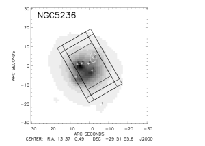
NGC 5236	13 37 00.50 $-$29 51 55.3	0.001721	5.0	$1.29\times 10^{10}$	HII		SAB(s), face-on, WR
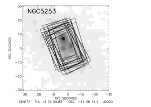
NGC 5253	13 39 55.80 $-$31 38 31.0	0.001348	4.1	$1.64\times 10^{9}$	HII		Im pec, BCD, WR
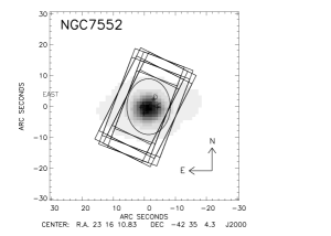
NGC 7552	23 16 10.80 $-$42 35 04.2	0.005287	21.2	$6.73\times 10^{10}$	HII, LINER		SBbc

2.2 Observations and Data Reduction

The ISO-SWS instrument on-board ISO performed spectroscopic measurements between 2.38 to 45.2$\mu$m with grating spectrometers producing spectra of medium to high resolution [R=1000-2000, see de Graauw et al. (1996); Leech et al. (2002) for more details]. Within its operational wavelength range lie a number of previously seldom-observed emission lines including fine structure line and H-recombination lines from which elemental abundances may be determined.

The ISO Data Archive was used to collate all of the SWS grating spectra available for each galaxy. Most data sets were taken using the SWS02 observation template, which provides medium resolution measurements of targeted lines. In some cases, full grating scans producing lower resolution spectra were taken (the SWS01 observations template) and a handful of medium resolution SWS06 measurements were also made. Where multiple observations were available, care was taken not to combine data taken with different aperture centres to ensure the same part of the galaxy was being measured for each observation.

We used the SWS interactive analysis (IA3) to reduce the data sets from the edited raw data products. The motivation for using IA3 to re-reduce the data (rather than the pipeline reduction) was to enhance the quality of the reduced product by using interactive tools for dark current subtraction, correction between up and down scans and outlier masking. The resultant reduced spectra were then subject to further processing in ISAP (Sturm et al. 1998) to remove further outliers and to perform flat-fielding and fringe removal (where necessary) to produce the final spectral line profiles from which line fluxes were measured. The reduced data will also be made publicly available through the ISO Data Archive.

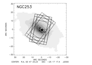
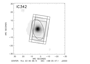
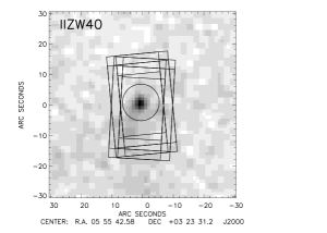
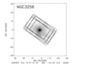
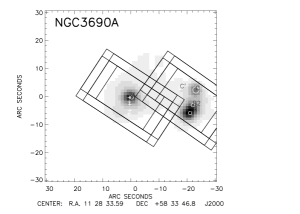
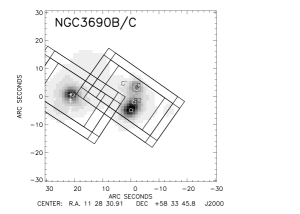
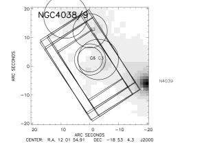
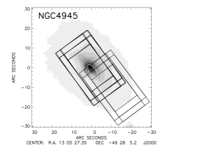
Since the ISO-SWS instrument takes measurements in a number of aperture size and detector combinations, aperture corrections should be considered for sources which are extended with respect to the apertures (of sizes $14"\times 20"$, $14"\times 27"$ and $20"\times 33"$ centred on the coordinates given in Table 1). As we are interested in emission from only the compact nuclear optically obscured infrared starburst we used radio, millimetre or infrared measurements from the literature to determine the starburst extent to compare to the ISO-SWS aperture (see Fig. 1 for details). We found no sources required correction for extension except M82. The corrections for this source are described in Förster-Schreiber et al. (2001).

Error propagation through the reduction of ISO-SWS data is described in Shipman et al. (2001) and Leech et al. (2002). To this error we add an additional 20% calibration error to account for systematic inaccuracies in the photometric calibration (Table 4.7 in Leech et al. 2002).

Figure 1: 2MASS quick-look postage stamps (log-scale) of the starbursts with SWS apertures (rectangular) overlaid. Additionally, overlaid ellipses indicate the extent of the starburst regions as obtained from the literature. Notes on individual sources: NGC 253 The MIR emission is dominated by a region of $\sim$10^′′ in size (Böker, Krabbe, & Storey 1998) and a single super-star cluster lying within it (Keto et al. 1999). IC 342 The central radio source is of comparable size to the SWS aperture (Hummel & Graeve 1990). II Zw 40 The 12$\mu m$ emission originates from a region only 0.5^′′ in diameter (Beck et al. 2002). M82 See Förster-Schreiber et al. (2001). NGC 3256 Has a compact double nuclei with combined angular size smaller than the SWS aperture (Norris & Forbes 1995) and is in agreement with the size ($<$10^′′ diameter) determined from MIR mapping at [NeII]12.8$\mu m$ and the N-band (Böker et al. 1997). NGC 3690A & B/C The discrete compact radio ad CO emitting sources are also the sites of strongest MIR emission - refer to images presented in Keto et al. (1997) and Soifer et al. (2001). The overlaid ellipses are the MIR source sizes determined by the latter authors. NGC 4038/9 The SWS aperture contains emission from SGMC2,3,4,5 as identified by Wilson et al. (2000). NGC 4945 N-band imaging reveals this source has a compact unresolved nucleus with surrounding core emission oriented along the galaxy’s major axis (Krabbe, Böker, & Maiolino 2001). The overlaid ellipse marks the extent of the gas emitting CO(2-1) lines from Ott et al. (2001). Data from the SWS aperture offset from the radio source are not included within the analysis in this paper. NGC 5236 The ellipse marks the starburst extent determined from radio maps from Turner & Ho (1994) (additional hotspots are also marked). NGC 5253 extent of [SIV]10.5$\mu$m emission from Beck et al. (1996) (but see also Gorjian, Turner, & Beck 2001). NGC 7552 The majority of the NIR and MIR flux originates from a circumnuclear starburst ring of $\sim$10^′′ in diameter (ring and hot spots are marked Forbes, Kotilainen, & Moorwood 1994; Schinnerer et al. 1997).

3 Results - The MIR spectroscopic survey of local starbursts

We present a survey of mid-infrared emission lines from a sample of infrared starbursts. The emission line fluxes for the most commonly detected lines within the range of the ISO-SWS instrument may be found in Table 2.

Our starburst sample encompasses a variety of morphological types (Table 1) and includes six starbursts exhibiting Wolf-Rayet spectral features (Schaerer, Contini, & Pindao 1999). From this list of Wolf-Rayet galaxies we exclude NGC 5236 since Rosa & D’Odorico (1986) detected Wolf-Rayet signatures only in regions centred upon three supernovae sites, none of which lie within our observation aperture. Recently, Bresolin & Kennicutt (2002) report on the possible detection of Wolf-Rayet-like features in the spectrum of a nuclear ‘hot-spot’ in NGC 5236. However, due to the weakness of the features, for the subsequent analysis, we assume the central region does not contain large numbers of Wolf-Rayet stars (see also Sect. 5.5).

Of our sources, only NGC 4945 displays evidence for harbouring an AGN. Spoon et al. (2000) have demonstrated that this AGN does not contribute to the flux of the mid-infrared emission lines. In addition, an AGN has been advocated to be responsible for the ionisation required to produce radio-recombination lines detected in NGC 253 (Mohan, Anantharamaiah, & Goss 2002).

We detect a number of fine structure lines within the ISO-SWS spectra. In particular, the fine structure transitions of singly and doubly ionised Ar and Ne are detected in the majority of sources as well as those of [S III] and [S IV]. Other commonly detected transitions are [O IV]25.89$\mu$m, [Fe II]26.0$\mu$m and [Si II]34.81$\mu$m. The majority of these lines are likely to have an origin in electron impact excitations in H II regions that have been photo-ionised by hot stars (assuming these sources are pure starbursts) with a possible contribution from fast ionising shocks. The [Si II] line is believed to partly originate in photodissociation regions (e.g. Sternberg & Dalgarno 1995) at the interfaces between H II regions and the surrounding dense molecular clouds. The ISO-SWS detected lines span a range of excitation potentials from 8.2eV for [Si II] to 55eV for [O IV]. The origin of the [O IV] transition in starburst and Wolf-Rayet galaxies is discussed in Lutz et al. (1998) and Schaerer & Stasińska (1999) respectively. In addition, the H-recombination lines Brackett $\alpha$, $\beta$ and Pfund $\alpha$ are detected in most of our galaxies.

We have also measured several transitions of molecular hydrogen. $H_{2}$ data for all the objects in our sample are included in the analysis of Rigopoulou et al. (2002). Our reductions use the newest calibration files of the ISO-SWS instrument and we find the majority of our fluxes are consistent within the calibration uncertainties of Rigopoulou et al. and therefore we do not present the $H_{2}$ line fluxes here. We also do not address the broad emission and absorption features due to dust and ice that are measured in M 82 and NGC 253. These are discussed by Sturm et al. (2000).

Table 2: Emission line fluxes (uncorrected for extinction), in units of $10^{-20}Wcm^{-2}$. Also given are the calculated $A_{V}$ for a mixed model with a Lutz (1999) extinction law and $log_{10}<Q(H_{0})>$ calculated as described in the text.

Line	$\lambda$($\mu$m)	NGC253	IC342	II Zw 40	M82	NGC3256	NGC3690A	NGC3690B/C	NGC4038	NGC4945	NGC5236	NGC5253	NGC7552
HI Brb	2.6260	14.7	3.4	1.2	41.0	4.2	2.1	2.1	0.8	—	4.8	2.7	2.5
HI Pfd	3.2970	2.6	—	$<$4.8	5.9	—	—	—	—	—	—	—	—
HI Pfg	3.7410	3.0	—	—	10.7	—	—	—	—	—	—	—	—
HI Bra	4.0520	31.2	7.0	2.6	81.5	4.4	2.6	3.7	2.5	9.9	7.8	4.5	4.4
HI Pfa	7.4600	7.6	2.4	$<$4.6	25.9	2.3	1.0	0.7	—	2.3	—	2.5	—
[MgVII]	5.5032	$<$7.1	$<$0.8	$<$16.8	$<$69.3	—	—	—	—	—	—	—	$<$1.1
[MgV]	5.6098	$<$3.1	—	$<$17.4	$<$79.2	$<$2.3	—	—	—	—	—	$<$1.7	—
[ArII]	6.9852	184.7	58.6	0.2	267.0	22.7	—	—	2.2	24.2	—	2.3	18.5
[NeVI]	7.6524	$<$0.6	—	$<$6.2	$<$49.5	$<$1.3	$<$0.4	$<$0.5	—	$<$0.7	—	—	—
[ArIII]	8.9913	7.0	2.6	2.0	47.6	4.7	1.3	2.8	1.8	$<$2.3	—	5.9	2.5
[SIV]	10.510	$<$3.3	$<$1.2	19.8	14.9	0.9	1.0	3.5	2.7	$<$0.9	0.9	34.0	0.3
[NeII]	12.813	453.6	90.7	1.7	714.0	89.2	31.9	27.7	7.7	92.5	133.9	7.9	68.0
[NeV]	14.321	$<$7.6	$<$0.7	$<$0.8	$<$29.7	$<$4.8	$<$0.5	$<$1.1	—	$<$0.5	$<$0.5	$<$0.3	—
[ClII]	14.367	7.7	0.7	$<$4.1	$<$33.0	$<$1.8	—	—	—	0.3	1.8	$<$1.5	—
[NeIII]	15.555	32.1	8.4	17.0	126.0	14.2	9.3	20.0	6.5	9.8	6.8	28.9	5.1
[SIII]	18.713	99.2	45.3	5.1	252.0	32.5	8.2	18.4	7.3	6.3	54.4	15.9	24.6
[FeIII]	22.925	17.1	—	—	46.6	3.3	—	—	—	0.7	—	—	—
[OIV]	25.890	6.7	0.7	1.1	8.0	0.8	0.6	1.0	$<$0.3	3.5	0.8	0.9	1.0
[FeII]	25.988	14.2	4.8	1.0	36.7	2.8	1.6	2.2	0.3	3.5	4.2	0.9	2.0
[SIII]	33.481	197.3	89.3	11.4	562.0	56.4	27.1	34.1	16.0	51.4	109.8	34.4	41.1
[SiII]	34.815	273.2	131.6	4.5	839.0	84.0	43.4	42.2	10.5	107.4	138.0	16.7	61.5
[NeIII]	36.013	$<$4.5	$<$2.3	1.4	18.8	2.4	$<$1.3	1.8	1.8	$<$1.6	1.0	4.9	$<$0.8
$A_{v}$		8.67	7.22	10.36	52.00	$<$8.73	38.94	$<$57.13	37.34	188.19	5.00	5.08	$<$73.90
$log_{10}<Q(H_{0})>$		53.02	51.94	53.77	53.83	54.53	54.62	54.76	53.81	53.61	52.90	52.34	54.40

4 Analysis

4.1 Extinction Correction

Several of our starburst galaxies are known to be dusty systems with large obscuration; therefore the observed line fluxes must be corrected for extinction. To determine the correction, we used the ratios of $Br\beta/Br\alpha$ and $[SIII]18.7/33.5$. The intrinsic emissivities of H-recombination lines are theoretically well determined and may be compared to the ISO-SWS measurements to determine the level of extinction. Moreover, ratios of H-recombination line emissivities are relatively insensitive to variations in electron temperature and density and therefore reasonable (rather than precisely accurate) estimates of the two quantities is sufficient to identify the appropriate intrinsic line ratio. Emissivity coefficients from Storey & Hummer (1995) for case B recombination with an electron temperature of $10^{4}$K and density of $100cm^{-3}$ were used to calculate the intrinsic line ratios for the H recombination lines. We chose not to use the H-recombination line ratio of $Br\alpha/Pf\alpha$ since Lutz (1999) suggest that the extinction at 7.5$\mu$m may be higher than predicted by standard extinction curves (Draine 1989), with the possibility of significant variation among sources.

The ratio $[SIII]18.7/33.5$ is more sensitive to density than the H recombination lines but there are good reasons to assume that the starbursts are close to the low density limit (Sect. 4.2.1). We solved the rate equations for this ratio using the updated atomic data of Tayal & Gupta (1999) and confirmed that the resulting ratio is relatively insensitive to temperature. We adopt a value of $0.5$ for densities close to the low density limit.

The extinction was calculated based upon a model in which obscuring material and emitting gas are uniformly mixed. Such a ‘mixed’ model is considered more appropriate for a starburst region observed with our large apertures than a simple foreground screen (McLeod et al. 1993). The attenuation of the emitted intensity may be expressed as

$$I=I_{0}\frac{1-e^{-\tau_{\lambda}}}{\tau_{\lambda}}$$ (1)

where $\tau_{\lambda}$ is the optical depth at the wavelength of interest ($\lambda$) which is proportional to the optical depth in the V band $\tau_{V}$ through the extinction law. We assumed the Galactic centre extinction law of Lutz (1999) between 3-8.5$\mu$m and adopted a Draine (1989) extinction law at all other wavelengths, with a normalisation of the silicate feature of $\tau_{9.6}/\tau_{V}=0.122$. When comparing two recombination lines, the observed ratio may be expressed in terms of $\tau_{V}$ using the appropriate emissivity and extinction values.

In the case that all lines of both ratios $Br\beta/Br\alpha$ and $[SIII]18.7/33.5$ were detected, we quote a weighted average of the calculated $A_{V}$. For sources where only one of these ratios was measured, the corresponding $A_{V}$ was adopted. For NGC3256, NGC3690B/C and NGC7552 both measured ratios were higher than the intrinsic ratios, implying $A_{V}=0$ which is unrealistic for our dusty starbursts. We attribute the greater than intrinsic ratios to the large errors on our flux measurements ($\sim 20\%$). Therefore, as no meaningful values for the extinction could be found for these sources, we replaced the measured ratio by the measured ratio minus its associated error to determine a one sigma limit on $A_{V}$. For these sources we apply an extinction correction using the one sigma limit of $A_{V}$ on the data but indicate the location of the uncorrected data ($A_{V}=0$) in the figures presented in the following sections. The estimated $A_{V}$ used to correct all line fluxes are given in Table 2.

4.2 Nebular Conditions

4.2.1 Electron density

To determine the electron density of our sources we used the ratios of [SIII]18.7$\mu$m/33.5$\mu$m and [NeIII]15.6$\mu$m/36$\mu$m and compared them to theoretical values obtained from a solution to the rate equations, obtaining relations of line ratios and densities close to those shown by Alexander et al. (1999), partly on the basis of earlier atomic data. Assuming a one-zone ionisation model, we found that all of our starbursts lie in the low density limit (i.e. well below the critical density) within the errors. Using only [SIII] both in the context of density indication and in extinction correction estimates (Sect. 4.1) allows degenerate low extinction/low density and high extinction/high density solutions. Low densities found from [NeIII] and general consistency of the recombination-line based and [SIII]-based extinction estimates assure however, that it is reasonable to adopt low density conditions for the entire sample. Our computations of collisional excitation indicate $n_{e}\sim 10-600cm^{-3}$ therefore we assumed an average electron density of $300cm^{-3}$. We were then able to use the expressions in the following section to calculate the nebular abundances in the low density limit (within which collisional de-excitation may be ignored).

4.2.2 Electron Temperature

As with density, electron temperature affects emissivities and thus inferred abundances albeit with only modest dependences for fine structure transitions and H-recombination lines. Since abundances are calculated as ratios of fine structure line to H-recombination line emissivities the weak dependence on electron temperature partly cancels out (e.g., Giveon, Morisset, & Sternberg 2002b). Accurate determinations of electron temperature can be obtained from recombination lines at radio and millimetre wavelengths. Measurements in the latter wavelength range are easier to interpret than in the radio since stimulated emission effects (which are present in the radio) are negligible and the millimetre line flux primarily originates in spontaneous emission. Therefore we sought electron temperature determinations based upon millimetre observations from the literature; for the starburst galaxies M82 and NGC 253, electron temperatures of $T_{e}\sim 5000K\pm 1000K$ have been determined by Puxley et al. (1989) and Puxley et al. (1997). An electron temperature estimate based upon radio recombination lines is also available for NGC 5253 (Mohan, Anantharamaiah, & Goss 2001), as well as estimates derived from optical spectroscopy for NGC 5253 and II Zw 40 (Campbell, Terlevich, & Melnick 1986; Vacca & Conti 1992; Walsh & Roy 1993). The results for these two objects agree well with the radio giving electron temperatures $\sim 10000-12500K$.

The known electron temperatures in our starburst regions span a factor $\sim$2 consistent with the well known correlation between electron temperature and metallicity (e.g. Campbell, Terlevich, & Melnick 1986, for a sample of on-average lower metallicity objects). For the remaining starburst galaxies, no accurate radio- or millimetre-based temperature determinations are available. We have chosen not to rely on electron temperature estimates derived from optical spectroscopy since these may not reflect electron temperatures of our obscured infrared-radio starbursts which cannot be probed by optical spectroscopy. For this reason, and to perform inter-comparisons between the sources without introducing a bias due to uncertain adopted electron temperatures, we elected to use a single ‘representative’ temperature for the entire sample of galaxies. Since M82 and NGC 253 are archetypal starbursts we chose our ‘representative’ electron temperature to be $T_{e}^{R}=5000K$. However, in doing so we appreciate that deviations from this ‘representative’ temperature are present and will affect absolute abundances, thus distorting the trends derived in the inter-comparisons. We will indicate these effects (which are largest for high $T_{e}$ objects) in the appropriate location. In particular for the BCD galaxies, the magnitude of the effect of using $T_{e}$ of $\sim 10000K$ on the abundances is shown in the relevant plots.

For consistency we have also adopted the same ‘representative’ electron temperature ($T_{e}^{R}=5000K$) for the H II regions from Giveon et al. (2002a), which we use as a comparison sample to the starbursts. We have re-calculated extinctions and abundances for this data set in order to eliminate any discrepancies due to different assumptions. The H II regions and starbursts are treated differently only in the obscuring model used to determine the extinction correction. For H II regions, often located in the Galactic plane but far from the Sun, we have adopted a uniform foreground screen model since we assume that extinction due to the foreground galactic ISM exceeds the extinction due to dust mixed within the ionised gas of the H II region itself. Similarly to the BCDs, the assumed representative temperature (5000K) is below the values that have been previously used [10000K (Giveon et al. 2002a), 7500K (Martín-Hernández et al. 2002a)]. Therefore the effect of increasing the temperature to 10000K shown on the figures in the next section is also applicable to part of the Giveon et al. (2002a) sample of H II regions, namely those at large Galactocentric radii or inside the Magellanic Clouds.

4.2.3 Lyman continuum photon emission rate

The Lyman continuum photon emission rate [$Q(H_{0})$] is the number of photons emerging per second from a star cluster with sufficient energies to ionise hydrogen. We have used H recombination lines to determine the average hydrogen ionising rate [$Q(H_{0})$] using

$$Q(H_{0})\sim\frac{L_{line}}{h\nu_{line}}\frac{\alpha_{B}(T_{e})}{\alpha^{eff}_{line}(T_{e})}.$$ (2)

The ratio of recombination coefficients ($\alpha_{B}/\alpha^{eff}_{line}$) is relatively insensitive to temperature (see equation 5.23 Osterbrock 1989). The recombination coefficients were taken from Storey & Hummer (1995). The calculated values of $Q(H_{0})$ are given in Table 2.

4.3 Excitation

Figure 2: Excitation diagnostic: $[NeIII]15.5/[NeII]12.8$ versus $[ArIII]8.9/[ArII]6.9$. Starbursts are plotted as filled squares with the Wolf-Rayet starbursts marked by an enclosing diamond. Galactic HII region data from Giveon et al. (2002a) are separated at the median galactocentric radius to provide ‘inner’ (open triangles) and ‘outer’ (open circles) samples. Finally, we plot the extragalactic H II regions from the same reference as open stars. The same key is used to distinguish the data points in all subsequent plots. Within this diagram low excitation is to the bottom-left quadrant and high excitation is to the top-right quadrant. All fluxes involved in this diagram were corrected for extinction. For NGC3256, NGC3690 B/C and NGC 7552 the effect of adopting $A_{V}=0$ on the derived quantities is plotted as an open square.

Figure 3: Excitation diagnostic: $[ArIII]8.9/[ArII]6.9$ versus $[SIV]10.5/[SIII]18.7$. Key as in Figure 2. Within this diagram low excitation is to the bottom-left quadrant and high excitation is to the top-right quadrant. All fluxes involved in this diagram were corrected for extinction.

Figure 4: Excitation diagnostic: $[NeIII]15.5/[NeII]12.8$ versus $[SIV]10.5/[SIII]18.7$. Key as in Figure 2. Within this diagram low excitation is to the bottom-left quadrant and high excitation is to the top-right quadrant. All fluxes involved in this diagram were corrected for extinction.

We may investigate excitation within the starburst sample using ratios of fine structure line fluxes of different ionic species of the same element (e.g. $X^{+i+1}/X^{+i}$). This ratio, to the first order and for a given ionisation parameter, is proportional to the number of photons which have sufficient energy to ionise the state $X^{+i}$ relative to the number of Lyman continuum photons. The difference in ionisation potentials between the ionic species means that ratios of these lines are sensitive to the shape of the spectral energy distribution (SED) of the ionising source. We have used (and combined) ratios of some of the strongest lines, $[NeIII]15.5/[NeII]12.8$, $[ArIII]8.9/[ArII]6.9$ and $[SIV]10.5/[SIII]18.7$, from our mid-infrared survey. Ar⁺, S⁺⁺ and Ne⁺ have ionisation potentials corresponding to $\sim 2$, $\sim 2.5$ and $\sim 3$ Rydbergs, respectively. Therefore these line ratios can constrain the ionising spectra over a range of a few Rydbergs.

We have formed diagnostic excitation planes by combining the fine structure line ratios as shown in Figs. 2, 3 and 4. The starbursts are relatively spread out across all three excitation planes. The majority of sources occupy the lower left corner of the planes, which indicates that these have low excitation. Extending to higher excitation in both axes are the BCD galaxies and those that exhibit Wolf-Rayet features (Wolf-Rayet galaxies are discussed in more detail in Sect. 5.5). This result is consistent with existing knowledge of both of these source types (Schaerer, Contini, & Pindao 1999).

Also plotted in the excitation planes are extinction corrected data of H II regions from Giveon et al. (2002a). The authors found an increasing excitation gradient with galactocentric radius within the galaxy (see also Martín-Hernández et al. 2002a; Giveon, Morisset, & Sternberg 2002b). Therefore these data have been separated into two broad bins based upon galactocentric radius (denoted by ‘inner’ and ‘outer’) and reflect low and high excitation. The distribution of the starbursts is well matched with the H II region data. The locations of the ‘inner’ H II regions is similar to those of low excitation starburst galaxies. The exceptions are the Wolf-Rayet and BCD galaxies which are located in regions similar to those of the ‘outer’ and extragalactic H II regions. These extragalactic H II regions have been heterogeneously selected from the Magellanic Clouds (Giveon et al. 2002a). The SMC and LMC are both low metallicity dwarf galaxies containing Wolf-Rayet stars and thus the coincidence of our Wolf-Rayet and BCD starbursts with the extragalactic H II regions is as expected.

For both the starbursts and the H II regions we see a general correlation between the three excitation ratios of Ne, Ar and S in Figs. 2-4. The existence of a correlation between all three ratios implies that they probe the same excitation mechanism. Moreover, the ratios are sensitive to photons emitted $\ga 2$, $\ga 2.5$ and $\ga 3$ Rydbergs and thus the correlations suggest that regions with ionisation potentials between $2-3$ Rydbergs in the ionising spectra, are likely to be closely related in ‘hardness’.

4.4 Elemental Abundances

In the following, we derive the elemental abundances for our sample galaxies and discuss their relation to other factors, in particular the role of metallicity in determining the wide range of excitations. Although we detect fine structure lines for several elements in some objects (Table 2), we restrict our abundance analysis to only those lines originating from H II regions and detected in the majority of sources within our sample i.e. neon, argon and sulphur, which are all thought to be ‘primary’ products of nucleosynthesis. They are products of oxygen burning, possibly in the late stages of evolution of massive stars (Garnett 2002). Thus the abundance of these primary products are likely to be correlated with the abundance of oxygen and should trace metallicity well.

4.4.1 Prescription

We calculate abundances using the following prescription. In general, the flux ($F^{X^{+i}}$) of a given ionic species ($X^{+i}$) may be written as the product of the number density of the ionic species ($n^{X^{+i}}$), the electron density of the ionised gas ($n_{e}$) and $j^{X^{+i}}$ - the emissivity of the species, i.e.,

$$\frac{F_{\lambda}^{X^{+i}}}{F_{\lambda}^{H^{+}}}=\frac{n^{X^{+i}}n_{e}j_{\lambda}^{X^{+i}}}{n^{H^{+}}n_{e}j_{\lambda}^{H^{+}}}$$ (3)

The ionic abundance ($n^{X^{+i}}/n^{H^{+}}$) may then be calculated from the flux ratio of the fine structure lines of an ionic species to a H-recombination line, multiplied by the ratio of the emissivities. In H II regions nearly all the hydrogen is ionised, therefore $n^{H+}\sim n^{H}$. The emissivity of the H-recombination line is obtained from the tables of Storey & Hummer (1995). Strictly speaking, the emissivities of ionic fine structure lines should be obtained by solving the rate equations for a full multilevel system under the appropriate conditions. However, for ground state fine structure transitions and a low density H II region, the following simple formula provides a good approximation

$$j_{\lambda}^{X^{+i}}=\sum_{u}\frac{hc}{\lambda}\left(\frac{8.629\times 10^{-6}}{T_{e}^{1/2}}\right)^{1/2}\left(\frac{\Upsilon_{lu}}{\omega_{l}}\right)e^{-\frac{\chi_{lu}}{kT_{e}}}$$ (4)

where $j$ has units of $erg\ cm^{3}\ s^{-1}$, $\Upsilon_{lu}$ is the effective collision strength, $\omega_{l}$ is the statistical weight of the lower level, $\chi_{lu}$ is the energy difference to the collisionally excited level from the ground state, and the summation is over those fine structure levels which, when collisionally excited from the ground state, decay through the line of interest. For the lines we used (Table 3), it is sufficient to consider one upper level only, with the exception of the [NeIII]15.5$\mu$m and [ArIII]9.0$\mu$m lines where two levels are needed. Effective collision strengths were obtained from the appropriate reference of the IRON project (Hummer et al. 1993, Table 3). The abundance of an ionic species may be calculated using

$$\frac{n^{X^{+i}}}{n^{H}}=\left[\frac{F_{\lambda}^{X^{+i}}}{F_{\lambda}^{H^{+}}}\right]\left[\frac{j_{\lambda}^{H^{+}}}{j_{\lambda}^{X^{+i}}}\right].$$ (5)

Once an ionic abundance has been estimated using the formula above (see Table 4), we sum the abundances for each ion from a given element and apply the ionisation correction factors (hereafter ICF) from Martín-Hernández et al. (2002a) to correct for the contribution from unobserved ionic species. The application of the ICFs from Martín-Hernández et al. (2002a) is appropriate for these data since we are using the same ionic species to determine the abundance, and the model grid used to calculate the ICFs is sufficient to include the sources similar to ours (i.e. those in the low density limit). Since the two dominant ionisation stages of Ne, Ar and S for H II region conditions are observed in our galaxies, the ionisation corrections factors are always close to unity. Following Martín-Hernández et al. (2002a), we do not correct our Ne abundances as the ICF is $\sim 1$ (see also Giveon et al. 2002a) and for S we applied a factor of 1.15. The ICF for Ar is seen to increase with excitation, from 1 to a maximum of 1.35. We interpolate over the factors calculated by Martín-Hernández et al. (2002a, Fig. 12) to obtain an ICF appropriate for the excitation (as determined from the Ne ratio) of each of our sources.

Table 3: Atomic data used to calculate the fine structure line emissivities and abundances. Effective Collision Strengths are interpolated to a temperature of 5000K. In addition the $Br\alpha$ recombination-line was used, adopting an emissivity of $\epsilon_{\lambda}^{Br\alpha}=2.298\times 10^{-26}ergcm^{3}s^{-1}$ from Storey & Hummer (1995) for $n_{e}\sim 100cm^{-}3$ and $T_{e}\sim 5000K$.

Line	Wavelength	$\Upsilon_{lu}$	$\omega_{l}$	$\chi_{lu}$	Reference for $\Upsilon_{ul}$
	($\mu$m)			(eV)
[NeII]	12.8136	0.277	4	0.09684	Saraph & Tully (1994)
[NeIII]	15.5551	0.730	5	0.07971	Butler & Zeippen (1994)
		0.199	5	0.11413	Butler & Zeippen (1994)
[ArII]	6.9853	2.70	4	0.17749	Pelan & Berrington (1995)
[ArIII]	8.9914	3.182	5	0.13789	Galavis, Mendoza, & Zeippen (1995)
		0.663	5	0.19469	Galavis, Mendoza, & Zeippen (1995)
[SIII]	18.7130	1.41	1	0.10329	Tayal & Gupta (1999)
[SIV]	10.5105	8.10	2	0.11796	Saraph & Storey (1999)

Table 4: Calculated elemental abundances for each source, per ionic species and the total (ICF corrected) abundance with reference to solar abundances ([X/H]): for Ne, Ar and S from Grevesse & Sauval (1998) (first line). The abundances presented are for $T_{e}=5000K$. See text for the effect of this assumption on the lowest abundances.

Name	$n^{Ne^{+}}/n^{H}$	$n^{Ne^{++}}/n^{H}$	[Ne/H]	$n^{Ar^{+}}/n^{H}$	$n^{Ar^{++}}/n^{H}$	[Ar/H]	$n^{S^{++}}/n^{H}$	$n^{S^{3+}}/n^{H}$	[S/H]
	$\times 10^{-5}$	$\times 10^{-6}$		$\times 10^{-6}$	$\times 10^{-7}$		$\times 10{-6}$	$\times 10^{-7}$	$\times 10^{-1}$
Solar			1.20e-04			2.51e-06			1.58e-05
IC342	$27.6\pm 8.7$	$10.9\pm 3.8$	$2.4\pm 0.7$	$12.1\pm 3.8$	$6.6\pm 2.6$	$5.1\pm 1.5$	$9.4\pm 3.0$	$----$	$6.8\pm 2.1$
II Zw 40	$1.4\pm 0.8$	$59.0\pm 20.8$	$0.6\pm 0.2$	$0.1\pm 0.1$	$14.6\pm 6.0$	$0.9\pm 0.3$	$2.9\pm 1.1$	$32.3\pm 10.8$	$4.4\pm 1.1$
M82	$17.0\pm 7.2$	$11.6\pm 4.9$	$1.5\pm 0.6$	$4.4\pm 1.9$	$15.8\pm 6.7$	$2.4\pm 0.8$	$4.3\pm 1.8$	$1.2\pm 0.5$	$3.2\pm 1.3$
NGC253	$31.0\pm 9.4$	$9.3\pm 3.1$	$2.7\pm 0.8$	$8.6\pm 2.7$	$4.1\pm 1.5$	$3.6\pm 1.1$	$4.6\pm 1.5$	$----$	$3.4\pm 1.1$
NGC3256	$43.2\pm 18.5$	$29.1\pm 13.1$	$3.8\pm 1.5$	$7.4\pm 3.3$	$19.3\pm 8.9$	$3.8\pm 1.4$	$10.7\pm 4.7$	$0.8\pm 0.5$	$7.8\pm 3.4$
NGC3690A	$23.8\pm 10.1$	$27.6\pm 11.7$	$2.2\pm 0.8$	$----$	$12.9\pm 5.5$	$0.5\pm 0.2$	$4.4\pm 1.9$	$2.4\pm 1.0$	$3.4\pm 1.4$
NGC3690B/C	$14.4\pm 6.1$	$40.2\pm 17.0$	$1.5\pm 0.5$	$----$	$21.1\pm 9.0$	$1.0\pm 0.4$	$7.0\pm 3.0$	$6.4\pm 2.7$	$5.5\pm 2.2$
NGC4038	$6.1\pm 2.6$	$20.3\pm 8.6$	$0.7\pm 0.2$	$1.2\pm 0.5$	$17.6\pm 7.5$	$1.4\pm 0.4$	$4.2\pm 1.8$	$6.6\pm 2.8$	$3.5\pm 1.3$
NGC4945	$17.2\pm 6.5$	$6.7\pm 2.6$	$1.5\pm 0.5$	$----$	$----$	$----$	$0.9\pm 0.4$	$----$	$0.6\pm 0.3$
NGC5236	$36.8\pm 15.6$	$8.0\pm 3.4$	$3.1\pm 1.3$	$----$	$----$	$----$	$10.1\pm 4.3$	$0.4\pm 0.2$	$7.4\pm 3.1$
NGC5253	$3.8\pm 1.7$	$59.4\pm 22.3$	$0.8\pm 0.2$	$0.7\pm 0.4$	$22.2\pm 9.0$	$1.5\pm 0.5$	$5.2\pm 2.0$	$28.1\pm 10.5$	$5.8\pm 1.6$
NGC7552	$29.5\pm 12.5$	$8.4\pm 3.6$	$2.5\pm 1.0$	$5.6\pm 2.4$	$16.3\pm 6.9$	$2.9\pm 1.0$	$7.9\pm 3.3$	$0.4\pm 0.2$	$5.7\pm 2.4$

4.4.2 The abundance of neon and argon

Figure 5: Excitation against abundance for neon. Starbursts are plotted as asterisks with the Wolf-Rayet starbursts marked by an enclosing diamond. Galactic and local-extragalactic HII region data from Giveon et al. (2002a) are also plotted as open triangles, circles and stars. For a given metallicity the starbursts are of lower excitation than the HII regions. The arrow indicates the effect on the abundances of changing the adopted electron temperature from 5000 to 10000 K.

Figure 6: Excitation against abundance for argon. Symbols are as in Fig. 5.

In Figs. 5 and 6 we show the relationship between excitation and abundance for Ne and Ar for the starburst sample. A trend of decreasing excitation with increasing abundance is clearly seen in Ne and Ar for the starburst regions. The Wolf-Rayet galaxies have the highest excitation and the lowest abundance. In general, the non-Wolf-Rayet starbursts in our sample have super-solar metallicities $(X/H)\sim 1-3(X/H)_{\sun}$ (where X is Ne or Ar) whereas the Wolf-Rayet and BCD galaxies are sub-solar. As discussed in Sect. 4.2.2, our adopted ‘representative’ electron temperature of 5000 K is a good assumption for high metallicity starbursts and high metallicity H II regions. However, the same is not true for the BCD galaxies and the lower metallicity H II regions among the sample of Giveon et al. (2002a). Therefore, the effect of changing the electron temperature from 5000 to 10000 K on the calculated abundances is shown with an arrow in the diagrams. By adopting a more appropriate electron temperature, the absolute infrared-derived abundances of the low metallicity BCDs are close to the optically-derived values [$0.2(X/H)_{\sun}$] (e.g. Hunter, Gallagher, & Rautenkranz 1982; Vacca & Conti 1992; Walsh & Roy 1993; Masegosa, Moles, & Campos-Aguilar 1994). Overall, the effect on the excitation/abundance diagram of Fig. 5 of adopting individual electron temperatures (which are unavailable for the entire sample) for each starburst would be to tilt the correlation: the high excitation / low metallicity end would move to $\sim$2 times lower abundance, while the high metallicity/low excitation end remains unchanged.

From the literature we found accurate electron temperatures for the infrared starburst regions of M82, NGC 253, II Zw 40 and NGC 5253 (as described in Sect. 4.2.2) which we used to re-calculate the elemental abundance of neon (Table 5) in these galaxies. II Zw 40 and NGC 5253 ($T_{e}\sim 12500K$ and $\sim 11000K$, respectively) lie at the low abundance, high excitation end of our abundance-excitation correlation, while M82 and NGC 253 ($T_{e}\sim 5000K$) lie at the opposite extremity. We then defined a linear relationship between excitation and true Ne abundance (calculated using the measured actual electron temperatures) defined by these two pairs of galaxies. We could then estimate neon abundances for the remaining galaxies in the sample by interpolating along this relation based upon their [Ne III]15.5/[Ne II]12.8 excitation ratios. This process yielded abundance estimates that are essentially independent of our knowledge (or lack thereof) the true electron temperature for each source. The estimated abundances (Table 5) for the low excitation sources are all close to $\sim 2Z_{\sun}$.

Table 5: Neon abundances for our sample of galaxies calculated assuming a fixed electron temperature of 5000K (column 2) and individual electron temperatures (3rd column). For the latter, abundances are derived from interpolating between objects with known electron temperatures (values indicated by bold face), on the basis of their [Ne III]15.5/[Ne II]12.8 excitation ratios.

Name	$[Ne/H](5000K)$	$[Ne/H](T_{e})$
IC342	2.4	2.1
II Zw 40	0.6	0.3
M82	1.5	1.5
NGC253	2.7	2.7
NGC3256	3.8	2.1
NGC3690A	2.2	2.0
NGC3690B/C	1.5	1.9
NGC4038	0.7	1.9
NGC4945	1.5	2.1
NGC5236	3.1	2.1
NGC5253	0.8	0.4
NGC7552	2.5	2.1

Figure 7: Left: [Ne/H] abundance vs. [Ar/H] abundance. The key is as in Fig. 2. Right: [Ar/Ne] abundance ratio vs. [Ne/H] abundance. The key is as in Fig. 2. In both panels, a dashed line represents the solar abundances and abundance ratios for these elements. The arrows marked ‘ISM’ and ‘Orion’ denote the effect on the data of using different reference abundances other than solar - ‘ISM’ interstellar medium from Wilms, Allen, & McCray (2000) and Orion abundances from Simpson et al. (1998). Adopting these different reference abundances only change the absolute values but not the correlation.

As ‘primary’ products of stellar nucleosynthesis, the abundances of neon and argon are expected to be correlated. The overall abundance relation between Ne and Ar is shown in Fig. 7 which indeed shows a clear correlation between the two elements that holds for all objects in our sample, from the BCDs and WR galaxies to the dusty starbursts. This implies that the ISM of these galaxies has been enriched by similar processes for both elements. The [Ar/Ne] ratio shown in the right panel (for which the $T_{e}$ effects for the two elements largely cancel) suggests an above solar average argon to neon abundance ratio with no obvious trend among the galaxies.

4.4.3 The abundance of sulphur

We discuss the abundance of sulphur separately since we do not see the clear correlation between excitation and abundance that is seen in Ne and Ar for the starbursts (Fig. 8). In addition, all galaxies appear to have sub-solar sulphur abundances, with NGC 4945 being anomalously low. Furthermore, on comparison to the abundances of Ne and Ar, we find that the galaxies not showing Wolf-Rayet features have lower S abundances ($<[S/H]>=0.6$) than expected from their typically high Ne and Ar abundances ($<[Ne/H]>=2.4,\ <[Ar/H]>=2.7$). Yet the S abundances for the Wolf-Rayet galaxies (which typically have lower Ne and Ar abundances) are similar to that expected from their Ne and Ar abundances ($[X/H]\sim 0.2$).

Figure 8: Excitation against abundance for Sulphur. Symbols are as in Fig. 5. Unlike the corresponding figures for neon and argon, no correlation is seen.

Figure 9: Left: [Ne/H] vs. [S/H] abundance. The key is as in Fig. 2. Right: [S/Ne] v [Ne/H] abundance. The key is as in Fig. 2. For both panels, dashed lines represents the solar abundance and abundance ratios.

Figure 10: Left: [Ar/H] v [S/H] abundance. The key is as in Fig. 2. Right: [S/Ar] v [Ar/H] abundance. The key is as in Fig. 2. For both panels, dashed lines represents the solar abundance and abundance ratios.

We confirm this result in Figs. 9 and 10, where we investigate the correlations between S abundances and Ne and Ar. S is also expected to be correlated with Ne and Ar since they are all primary products of stellar nucleosynthesis. However, we see no correlation between the abundances of S in the galaxies with either Ne or Ar. The right panels of Figs. 9 and 10 compare the abundance ratios [S/Ne] and [S/Ar] with the Ne and Ar abundance. They reflect the trend towards a stronger sulphur ‘deficiency’ at increased Ne or Ar abundance noted above. S is often referred to as an excellent tracer of metallicity (e.g. Oey & Shields 2000) and in studies of the ISM is commonly used as a non- or slightly-depleted ($\la 30\%$) element (e.g. Wilms, Allen, & McCray 2000). However, the significant underabundance of S implied by the results of this study clearly has implications for the use and interpretation of sulphur fine structure lines and sulphur abundances in starburst sources. This result suggests that S is not a good tracer of metallicity in starburst galaxies. We discuss possible explanations for this depletion of sulphur below.

5 Discussion

5.1 Comparison to optical/NIR derived abundances

A direct comparison to the abundances derived from optical/NIR studies is far from straightforward. In particular, our obscured starbursts are not directly comparable to optical derived abundances since the regions we are probing may be completely obscured. Moreover, when making comparisons for our sources of large angular size one must ensure that the spectra in both regimes are probing the same regions.

The abundances obtained from our infrared study complement optical/NIR determinations by adding Ne, Ar and S which have predominant excitation species in the mid-infrared wavelength range. We searched the literature for abundances determined from optical spectroscopy for these elements, or for oxygen with which they are expected to be correlated. For II Zw 40 and NGC 5253, optical based abundances are consistent with our mid-infrared results ($Z\sim 0.2Z_{\sun}$ Kobulnicky et al. 1997). For our low excitation starbursts with metallicities close to $2Z_{\sun}$, while optically derived values are in agreement that the starbursts have super-solar metallicities, the estimates are slightly discrepant with our infrared determinations. For NGC 3256 (Bresolin & Kennicutt 2002, and references therein) and NGC 7552 (Storchi-Bergman, Calzetti & Kinney 1994) the derived metallicities are slightly lower $Z\sim 1.5Z_{\sun}$, whereas for N5236 the determinations is slightly higher $Z\sim 2.6Z_{\sun}$ (Storchi-Bergman, Calzetti & Kinney 1994).

5.2 Excitation and Abundance

The strong negative correlations seen for Ne and Ar in Sect. 4.4.2 indicate that ‘spectral hardness’ of the ionising stars is inversely correlated with metallicity. This correlation is likely to arise from several factors, such as: (a) The influence of metallicity on stellar atmospheres and the resulting stellar spectral energy distribution, for a given effective temperature of the star. (b) Variations of stellar evolutionary tracks with metallicity. (c) Variations of IMF with metallicity. The observed spread of the correlation could result from variations in the electron temperature, starburst age and the IMF among sources in our sample. We discuss the causes of both the correlation and the scatter in this section.

Theoretical models of hot star atmospheres indicate that metallicity variations affect stellar wind strengths and, therefore mass-loss rates, as a result of changes in the opacity in the line-driven winds. Changes in metallicity also induce changes in the the effects of line blocking and blanketing. Thornley et al. (2000) and Giveon et al. (2002a) present a discussion of the effects on stellar populations. Giveon et al. find that the increase in excitation of Galactic H II regions with galactocentric radius cannot be due to this effect alone [(a) in the list above]. Increasing effective temperatures must strongly contribute, in addition to the hardening of stellar SEDs for fixed $T_{eff}$. The same can be concluded for our galaxies by comparing the observed spread in excitations to the Giveon et al. models.

The effective temperature of a star-forming cluster is determined by at least three related factors: age, IMF, and metallicity. While we cannot differentiate between the individual effects of these three parameters on our data for single objects, we can discuss the influence they may have on our abundance-excitation correlations. Stellar evolutionary tracks across the H-R diagram also clearly display a dependence on metallicity (e.g., Schaller et al. 1992). For example, lower metallicity tracks have a ‘hotter’ main sequence. This explains why high excitation regions are found primarily at low metallicity (as Z varies from $Z_{\sun}$ to $0.2Z_{\sun}$ the observed Ne excitation ratio increases by factors $\sim 4-10$, Thornley et al. 2000). Evidence for the Galactic Centre may suggest this effect (b) is even stronger (see discussion in Thornley et al. 2000).

The question of whether (c) the IMF may vary among clusters of different metallicities remains open. Following arguments as in Thornley et al. (2000) we consider such IMF variations a minor contributor to our correlations. They showed that effects of moderate IMF slope variations on the excitation are not large, and discussed evidence in favour of the most massive stars being present in the initial mass function of objects for a wide range of metallicities.

We have already noted that some of our sources (particularly the BCDs) have measured electron temperatures that differ from the representative value of $T_{e}^{R}=5000K$. However, it seems unlikely that variations in $T_{e}$ could cause a correlation between ‘hardness’ (effectively $T_{eff}$) and metallicity, as the dependence of abundance on electron temperature is weak ($T_{e}^{-0.7}$ Giveon et al. 2002a). If $T_{e}$ increases with metallicity, as is suggested by the electron temperatures we found for NGC 253, M82, II Zw 40 and NGC 5253, then the variations in $T_{e}$ for our sample of galaxies will affect the slope of the correlation we find between ‘hardness’ and metallicity, but will not destroy it. In the unlikely case that $T_{e}$ does not systematically vary with metallicity, then the variations in $T_{e}$ in our sample will serve only to increase the spread in the correlation.

The observed scatter in the correlation may also result from differences in both starburst ages (as argued by e.g. Thornley et al. 2000; Giveon et al. 2002a) and the IMF for different star-forming clusters.

5.3 Comparison to H II regions

We also note from our ‘hardness’-metallicity plots, that for a given metallicity, the starbursts have relatively lower excitation than the H II regions. Similarly low excitations have been noted in previous studies of extragalactic star-forming regions (Doyon, Joseph, & Wright 1994; Doherty et al. 1995; Thornley et al. 2000). Our improved empirical database of starbursts (this paper) and H II regions (Giveon et al. 2002a), reinforces this result.

The low excitation of galaxies has been attributed to low upper-mass-cutoffs ($<30M_{\sun}$) and ageing effects (Thornley et al. 2000). The starbursts in our sample represent complex starburst systems with possibly multiple stellar populations lying within the SWS aperture, rather than the single stellar populations that comprise H II regions. This difference may account for the low excitation since the SWS aperture may include emission not only from the ‘youngest burst’ population but also from older stars within the host galaxy. The net effect of this ‘dilution’ is to lower the mean effective temperature of the starburst, which will result in the starbursts having lower ‘hardness’ ratios (cf Fig. 5 in Martín-Hernández et al. 2002b). This lowering of the mean effective temperature may mirror the effect of an ageing stellar population (as predicted by Thornley et al. 2000) on the observed line ratios.

5.4 Weak sulphur lines and the origin of low sulphur abundance

We have shown in Sect. 4.4.3 that the gas phase sulphur abundances do not follow the consistent behaviour seen in neon and argon. With the exception of the low metallicity systems, the measured S abundance is consistently smaller than that of Ne or Ar, by up to an order of magnitude in the metal-rich and dusty objects. In addition to the question of the origin of this deficit, the weakness of the S lines has practical implications for future observations of dusty starbursts both locally and at high redshift: sulphur lines are less favoured in comparison to the [Ne II] line as tracers of starburst emission than one would assume from nebular models. Instead of photoionisation models, empirical templates may be the tool of choice for flux predictions. Genzel et al. (1998) showed that low redshift ultraluminous infrared galaxies follow the trend of weak S lines relative to Ne, with Arp 220 being the most pronounced example.

Previous studies of Galactic H II regions also found low S abundances. From infrared spectroscopy, Simpson & Rubin (1990), Simpson et al. (1995) and Simpson et al. (1998) derived S and Ne abundances corresponding, on average, to a subsolar ratio of S/Ne, and suggested depletion of sulphur onto grains as a possible cause. This S deficiency was recently put on a much firmer observational basis by Martín-Hernández et al. (2002a), who used ISO observations of a larger sample to discuss Galactic abundance trends. Compared to the Ne and Ar abundances (with mean values similar to solar), their derived sulphur abundances are more scattered and are lower than solar by a factor $\la$3. For individual, higher-than-solar-metallicity extragalactic H II regions, Diaz et al. (1991) suggested a low S/O abundance ratio based on optical ($<1\mu$m) spectroscopy, but they emphasised the difficulty of determining abundances for high metallicity regions using optical data. These difficulties also apply to a possible Ar/O deficit at high metallicity (Garnett 2002), and are further reflected in the fact that other optical studies do not suggest a low S/O or Ar/O ratio for super-solar oxygen abundances (van Zee et al. 1998).

For the low S/H abundances measured in Galactic H II regions, Martín-Hernández et al. (2002a) propose an explanation involving uncertainties in electron temperature and density. While such uncertainties clearly exist, two arguments suggest that they are of secondary importance for the galaxies in our sample. First, the density measured from the [S III] lines is low for all galaxies in our sample and does not show the occasional high values that call the applicability of the low density approximation for determination of the S abundance in compact H II regions into question. Second, in addition to the inherently small temperature sensitivity of abundance determinations from fine structure lines, the remaining abundance variations caused by variations in temperature are expected to correlate among the three elements S, Ar, and Ne. Varying the adopted electron temperature from 5000 to 12500 K decreases the inferred abundances by factors of 2 to 2.5 for all three elements simultaneously. Large temperature uncertainties therefore should not selectively lower the sulphur abundance and increase the scatter in excitation versus abundance for sulphur alone, but rather affect all three elements similarly. In contrast, observations single out sulphur as being peculiar both in our data and in the H II region data of Martín-Hernández et al. (2002a) (their Figs. 18 and 19).

Another issue relevant to the question of S abundance is the ionisation correction factor used to compute the total sulphur abundance. Since the S underabundance occurs in low excitation objects, the missing fraction are unlikely to exist in higher ionisation stages (i.e. beyond the 47eV ionisation potential of $S^{3+}$) but more realistically in $S^{+}$ (23eV). However, the ICF calculations of Martín-Hernández et al. (2002a) show this effect to be small for the excitation range of our objects.

We consider a direct nucleosynthesis explanation of the sulphur deficiency to be unlikely. Neon, argon and sulphur are all primary elements expected to trace each other reasonably well. Variations will be related to the different stellar mass ranges contributing to the yields for each element. Extreme assumptions for the initial mass function, and/or variations of stellar lifetimes with mass, can influence the ratio of neon and sulphur abundances, since these two elements are produced mostly in supernovae with high (neon) and lower mass (sulphur) progenitors, respectively (Woosley & Weaver 1995). However, argon is produced over a very similar mass range as sulphur. Therefore, the observed abundance pattern of both neon and argon being ‘normal’, but sulphur being anomalously low by a large factor cannot easily be explained by differences in the mass ranges of the SNe.

The calculated elemental abundances are also heavily dependent upon the atomic data and therefore errors in the published values might be responsible for erroneous sulphur abundances. However, we have used the most recently determined collision strengths for both doubly and triply ionised S from Tayal & Gupta (1999) and Saraph & Storey (1999), respectively. These papers use improved and more complex methods to determine accurate collision strengths than previous, commonly used studies (e.g. Galavis, Mendoza, & Zeippen 1995; Johnson, Kingston, & Dufton 1986). While we identify atomic data as a possible contributor to the sulphur underabundance problem, the abundances we present are correct with respect to the most up-to-date atomic data available.

A consistent explanation of both extragalactic and Galactic observations would be a tendency of sulphur to be more strongly depleted onto dust than the noble gases neon and argon. However, ultraviolet absorption measurements in the diffuse interstellar medium often suggest most sulphur exists in the gas phase (Savage & Sembach 1996) with low depletion ($\sim 30\%$ Whittet 1984; Wilms, Allen, & McCray 2000). Other ultraviolet ISM studies suggest a correlation between sulphur depletion and mean hydrogen density (Gondhalekar 1985; Harris & Mas Hesse 1986; van Steenberg & Shull 1988), with depletions reaching a factor of 10 for lines of sight with mean hydrogen densities $\sim 1cm^{-3}$. For molecular regions, strong sulphur depletion is predicted by chemical models (e.g. Duley, Millar, & Williams 1980; Prasad & Huntress 1982; Ruffle et al. 1999). Unfortunately little is known about the H II regions probed by our observations beyond the infrared studies cited above. While depletion is a natural explanation of the failure of the S abundance data to trace the noble gas abundances, a quantitative understanding under the conditions of our higher than solar metallicity H II regions remains to be obtained. Clearly, depletion would have to depend on ISM conditions to explain both the low metallicity dwarfs (with no S deficit both from our results and numerous optical studies) and the higher metallicity starbursts. While noting these open questions, we consider depletion of sulphur onto grains the best explanation for our observations.

5.5 Wolf-Rayet Galaxies

Wolf-Rayet galaxies exhibit signatures of Wolf-Rayet stars in their integrated visible spectra and have been detected in a variety of galaxy types (e.g. BCDs, H II galaxies, AGN, LINERs etc.) but not in all objects of a particular class (Schaerer, Contini, & Pindao 1999). In general, the detection of Wolf-Rayet signatures in a galaxy has been interpreted as an indicator of young burst age ($3\la t_{sb}\la 8Myr$) and the presence of massive stars ($M_{upp}\ga 20M_{\sun}$), since the progenitors of Wolf-Rayet stars are postulated to be massive O stars. The Wolf-Rayet stage is thought to appear for a short time during the evolution of a simple stellar population.

In our sample, Wolf-Rayet galaxies are clearly separated from non-Wolf-Rayet galaxies. Wolf-Rayet galaxies generally have higher excitation and lower abundances than non-Wolf-Rayet objects. The current inventory of Wolf-Rayet features in external galaxies (Schaerer, Contini, & Pindao 1999) is definitely not unbiased, but in general Wolf-Rayet signatures have been detected mostly in low metallicity systems. The low detection rate of Wolf-Rayet stars in high metallicity systems is contrary to expectations from stellar evolution theory (e.g. Meynet 1995). Leitherer & Heckman (1995) for example, model the ratio of Wolf-Rayet stars to O stars in evolving starbursts using the Geneva tracks, and derive an order of magnitude increase in the metallicity range 0.25 to 2 $Z_{\sun}$; this range approximately corresponds to the metallicity spread in our sample.

Recent surveys of a large number of H II regions (Bresolin & Kennicutt 2002; Castellanos, Diaz, & Terlevich 2002; Pindao et al. 2002) located in the disks of local high metallicity galaxies have revealed the presence of weak Wolf-Rayet-like features in $\sim 30\%$ of the surveyed regions, which implies that Wolf-Rayet stars do in fact exist in high metallicity environments. This result confirms previous work on smaller samples (Guseva, Izotov, & Thuan 2000; Schaerer et al. 2000) and high metallicity systems included in other Wolf-Rayet samples (e.g. NGC 3049; Vacca & Conti 1992).

Yet, in highly obscured star forming regions, the presence of Wolf-Rayet stars remains to be confirmed. Our higher metallicity, non-Wolf-Rayet starbursts are all well studied and strong Wolf-Rayet features would not have escaped detection. NGC 5236 is the only exception. Despite its location in the excitation and abundance plots that is clearly consistent with the non-Wolf-Rayet starbursts, Bresolin & Kennicutt (2002) have recently identified possible Wolf-Rayet features in the optical spectrum of a nuclear hot-spot (hot-spot M83-A in their paper) which lies within our ISO-SWS aperture. The red and blue spectra they present have relatively low signal-to-noise and show no C IV$\lambda$5808 emission but do show a weak ‘blue-bump’ around 4650Å which is indicative of the presence of WN stars. Nevertheless, it is unlikely that the blue bump is solely due to WN stars. NGC 5236 has a N III $\lambda$4640 / He II $\lambda$4686 line ratio that is greater than unity which Schmutz & Vacca (1999) have shown cannot be reproduced by mixtures of known Wolf-Rayet stellar spectra. Schmutz & Vacca suggest that a large contribution from Of stars could also produce such emission features. Similar line ratios have also been found in other high metallicity systems (see Schaerer et al. 2000).

The separation of NGC 5236 with respect to II Zw 40 and NGC 5253 is not unexpected since they represent two very different classes of object. NGC 5236 is large barred spiral galaxy which is actively forming stars on kiloparsec scales, whereas for II Zw 40 and NGC 5253 the majority of star-formation and IR emission is thought to originate in 1 to 4 super-star clusters (c.f. Gorjian, Turner, & Beck 2001; Beck et al. 2002). Thus its location amongst the non-BCD galaxies is reasonable.

There could be several reasons for the non-detection of Wolf-Rayet features in most of our high metallicity objects: a special star formation history (no significant part of the population currently being in the brief Wolf-Rayet phase); dust obscuration of the regions actually hosting WR stars; and/or changes in spectral signatures of Wolf-Rayet stars at higher metallicity.

We do not consider fine-tuned star formation histories to be the dominant reason for the dichotomy in our sample. It seems very unlikely that only metal-rich objects are observed at extremely young or late ages (and with O stars still present to power the starburst). Circumventing this problem by postulating that the metal-rich objects are fully self-enriched in the current (almost terminated) burst would similarly require stringent assumptions on timing and the enrichment process. Most importantly, attempts using all available constraints for a detailed reconstruction of the star formation history in M 82, the prototype non-Wolf-Rayet object in our sample, predict a major part of the burst population to be in the ‘Wolf-Rayet phase’ (Rieke et al. 1993; Förster-Schreiber et al. 2002).

Obscuration of the regions hosting Wolf-Rayet stars is likely to be a significant effect. The presence of Wolf-Rayet stars is indicated by weak stellar emission features around 4650Å. In several of our objects, the most active star forming regions are considerably dust-obscured, and in the absence of convincing near or mid-infrared Wolf-Rayet tracers (Lumsden, Puxley & Doherty 1994), detection of any ‘classical’ optical Wolf-Rayet features is difficult. This is especially true if other, less obscured regions dilute the blue part of the visible spectrum. This is the case for M 82 which has a strong post-starburst component in its optical spectrum (e.g. Kennicutt 1992). It is worth noting that the high metallicity H II regions within which optical Wolf-Rayet features have been detected (Bresolin & Kennicutt 2002; Castellanos, Diaz, & Terlevich 2002; Pindao et al. 2002) are located within the disks of their host galaxies, and may suffer less extinction (and dilution) than our deeply obscured infrared star forming regions.

The role of Wolf-Rayet stars in metal rich starbursts also depends on still uncertain elements of the post main sequence evolution of massive stars. This is true for both the details of the evolutionary tracks, and the assignment of spectra to those tracks. For example, the ionising spectra of Wolf-Rayet stars may not be as hard as commonly assumed; this has implications for the spectra of composite starburst populations (Bresolin, Kennicutt, & Garnett 1999; Crowther et al. 1999; Bresolin & Kennicutt 2002). Additionally, evidence suggests that Wolf-Rayet stars in higher metallicity environments display different spectral signatures and weaker lines in the visible, compared to those in lower metallicity environments (Massey & Johnson 1998). Recent modelling by Bresolin & Kennicutt (2002) shows that Wolf-Rayet photons have a negligible contribution to the nebular ionisation as they are absorbed in the stellar atmospheres. The presence of Wolf-Rayet stars in our galaxies could be reflective only of young age. Moreover, in the Galactic centre Thornley et al. (2000) found that the majority of ionising flux originates from fairly cool (20000 to 30000 K) supergiants rather than the main sequence and hot Wolf-Rayet stars expected from a direct interpretation of the Geneva tracks. All this warns that a direct transfer from theoretically predicted Wolf-Rayet star numbers to observed signatures in high metallicity environments is currently difficult.

We note that the dichotomy between Wolf-Rayet and non-Wolf-Rayet objects in our sample could also be enhanced by an overestimation of the role of Wolf-Rayet stars in the low metallicity objects. Recent studies suggest the existence in very young star forming regions of non-Wolf-Rayet (core hydrogen burning) stars that, nevertheless, show Wolf-Rayet-like broad emission (Massey & Hunter 1998). This might additionally enhance the incidence of ‘Wolf-Rayet features’ among the very youngest, highest excitation objects (Schmutz & Vacca 1999).

6 Conclusions

We have presented mid-infrared spectral line data from a spectroscopic survey of a sample of starburst galaxies as seen by ISO-SWS. These data can be used as a reference database for comparison to future observations of star-forming galaxies with infrared telescopes such as SIRTF, SOFIA and Herschel.

From this database we have investigated the excitation and abundances of the sample using fine structure lines of the primary nucleosynthetic products neon, argon and sulphur and the H-recombination lines Brackett $\alpha$ and Brackett $\beta$. Abundance and excitation are inversely correlated for Ne and Ar. In addition, a comparison to local H II regions shows that for a given metallicity starbursts are of relatively lower excitation than the H II regions. The excitation of mid-infrared starburst spectra is hence governed by a combination of metallicity and other effects like ageing of the population, which should be accounted for in modelling starbursts as composite H II regions.

An analysis of the excitation and abundance as traced by fine structure lines of of sulphur indicates that sulphur is approximately 3 times underabundant for the low excitation metal-rich galaxies relative to Ne and Ar with which it should be correlated since it is also a primary product of nucleosynthesis. We favour depletion onto dust grains as the most likely cause of this relative underabundance. The weakness of the sulphur lines may favour neon as an indicator of star formation in future infrared spectroscopy of faint galaxies. In addition the derived low sulphur abundances imply that S is not a good tracer of metallicity.

Our sample displays a dichotomy between galaxies showing Wolf-Rayet features in the optical, which are of high excitation and low metallicity, and those without Wolf-Rayet features, which are of low excitation and high metallicity. This is opposed to the expectation of higher Wolf-Rayet fractions at higher metallicity from stellar evolutionary models. The most plausible reasons for this behaviour include obscuration coupled with a lack of convincing mid-infrared Wolf-Rayet tracers, dilution by less obscured regions in the optical spectrum and changes in the spectral signatures of Wolf-Rayet stars at higher metallicity.

The excitation probed by fine structure lines reported in this paper have been combined with those from a sample of active galaxies and are presented in a related paper (Sturm et al. 2002). Sturm et al. have constructed infrared analogues to the classical optical excitation diagnostics of Veilleux & Osterbrock (1987). The results show a clear separation between the two populations and the new excitation diagnostic can be used to identify powering mechanisms of obscured sources detected in future infrared surveys.