Design, Implementation and Testing of the MAP Radiometers

Abstract

The Microwave Anisotropy Probe (MAP) satellite, launched June 30, 2001, will produce full sky maps of the cosmic microwave background radiation in 5 frequency bands spanning 20 - 106 GHz. MAP contains 20 differential radiometers built with High Electron Mobility Transistor (HEMT) amplifiers with passively cooled input stages. The design and test techniques used to evaluate and minimize systematic errors and the pre-launch performance of the radiometers for all five bands are presented.

1 Introduction

This paper describes the design, implementation and testing of the microwave radiometers and support electronics incorporated in the Microwave Anisotropy Probe (MAP) satellite. The MAP mission is the second in NASA’s Medium-class Explorers (MIDEX) program (Bennett et al., 2003). Its purpose is to produce multi-frequency full sky maps of the microwave sky, from which maps of the cosmic microwave background radiation (CMB) can be extracted. The design of MAP is the result of a detailed study which involved balancing the mission’s three major interdependent performance requirements, angular resolution, sensitivity and systematic error suppression, while remaining consistent with the resources provided by MIDEX program. Some of the major design parameters which resulted are: angular resolution of $\approx 0\mbox{${\hbox to0.0pt{.\hss}}^{\circ}$}25$; minimally correlated pixel noise; full sky coverage; frequency coverage of $20-106\;\mbox{$\textrm{GHz}$}$  in 5 bands; polarization sensitivity; calibration accuracy better than $0.5\;\%$; sensitivity of $\approx 30\;\mbox{$\mu\textrm{K}$}$ per $3.2\times 10^{-5}$ sr/pixel.

The MAP instrument is composed of 20 differential HEMT based radiometers coupled to the sky by a set of back-to-back off axis Gregorian optics. The optics and input stages of the radiometers are passively cooled by radiation to space. The angle subtended between the two input beams of each radiometer is $\approx 140^{\circ}$. MAP observes from the second Earth-Sun Lagrange point using a compound spin motion producing highly interconnected scan patterns on the sky. These patterns greatly facilitate reconstruction of the temperature maps from the measured differential signals while suppressing systematic errors. Details of the entire mission, including diagrams of spacecraft and instrument layout and estimated uncertainties in the measured angular power spectra are presented in Bennett et al. (2003).

Control of possible sources of systematic errors (features in the maps, other than random noise, which are not present on the sky) was a high priority and greatly influenced many aspects of MAP’s design. Systematic errors can arise from several sources, including sidelobe pickup from foreground objects (the Sun, Moon, Earth and Galaxy), instrument instabilities (amplifier gain fluctuations, thermal drifts, etc.) or the data processing used to convert the time ordered data into calibrated sky maps. Careful optical design (Page, 2003; Barnes, 2002) orbit selection, and a scan strategy that keeps most contaminating sources far from the lines of sight of the instrument were used to minimize sidelobe pickup of foreground objects . The data processing procedure was checked for possible systematic errors by processing simulated data sets through the entire data processing pipeline and comparing the outputs to the simulation inputs.

Instrumental effects include instabilities inherent in the radiometers and those caused by environmental changes to the instrument. Intrinsic radiometer instabilities were minimized by the use of a differential radiometer design, the details of which are presented later in this paper. The entire observatory, comprising the instrument and spacecraft structure, was carefully designed to maintain as stable an environment as possible for the instrument. Specific examples are the scan strategy, which maintains a constant angle of insolation on the observatory, thermal isolation of the instrument from the spacecraft bus, and the nearly constant spacecraft power dissipation, all of which minimize thermal disturbances which could influence instrument performance.

A systematic error budget was established before the instrument build and estimates of contributions from all known potential signal sources were tracked throughout the program. Signal sources were classified as either spin synchronous or random. Random signals are those which are uncorrelated with orientation of the observatory. Random signals tend to average to zero, only the residual terms contribute to errors in the final maps. Spin synchronous signals, such as Galactic pickup from side-lobes or radiometer drifts due to spin synchronous thermal fluctuations do not average to zero, and therefore must be limited to much smaller values in the time ordered data. MAP is designed to limit the magnitude of systematic errors signals to less than $4.5$ $\mu\textrm{K}$ RMS in the uncorrected sky maps. Simulations indicate that spin synchronous artifacts in the time ordered data are suppressed by a factors of 2 or more by the map making algorithm given our scan pattern, so the corresponding allowed spin synchronous systematic error level in the time stream is $9$ $\mu\textrm{K}$. Of this a $2.6$ $\mu\textrm{K}$ contribution is budgeted for emission from cryogenic components in the feed horns and optical system, $2.8$ $\mu\textrm{K}$ from the radiometers, data collection system, and supporting electronics, with the remainder allocated to emission sources external to the satellite picked up by the side-lobe response of the optical system.

The MAP radiometers were designed to meet the systematic error requirement without applying any corrections to the radiometric data. The ultimate goal of these efforts is to produce high-quality sky maps with negligible striping along the scan directions and nearly diagonal pixel-pixel noise correlation matrices.

2 Radiometer Design

2.1 Overview

MAP contains 20 differential radiometers covering 5 frequency bands. They are direct conversion radiometers (no mixing to an intermediate frequency) and share the same basic design. Operation of the radiometers is similar to the continuous comparison radiometer described by Predmore (1985). Amplification is provided by High Electron Mobility Transistor (HEMT) amplifiers, with the input stages passively cooled to $\approx 90$ K to lower the system noise. The total microwave gain of each radiometer was selected so that the power input to each diode detector would be $\approx-23$ dBm during science observations. The resulting signal level is low enough to keep the diode detectors in the square law regime, but high enough so that intrinsic detector noise, and that added by the post detection electronics, degrade radiometer sensitivity by $<0.5\%$.

A total power radiometer’s sensitivity can be described by the radiometer equation (Kraus, 1986; Dicke, 1946) ,

$$dT=T_{\mathrm{sys}}\sqrt{\frac{1}{\Delta\nu_{\mathrm{eff}}\ \tau_{\mathrm{int}}}+\left(\frac{\Delta G}{G}\right)^{2}},$$ (1)

which relates the radiometer noise, $dT$, for an integration period $\tau_{\mathrm{int}}$, to the input referenced system noise temperature, $T_{\mathrm{sys}}$, and the effective RF bandwidth of the radiometers, $\Delta\nu_{\mathrm{eff}}$, given by

$$\Delta\nu_{\mathrm{eff}}=\frac{[\int G(\nu)d\nu]^{2}}{\int[G(\nu)^{2}]d\nu}$$ (2)

where $G(\nu)$ is the frequency dependent power response of the radiometer. The second term under the radical in equation 1 is the fractional power gain variation of the radiometer on the time scale of the integration, and would vanish for an ideal radiometer system.

The low noise and wide bandwidth of HEMT amplifiers make them strong candidates for use in the measurement of continuum signals, such as the CMB radiation. Unfortunately these amplifiers exhibit small fluctuations of their microwave gain with an approximate ‘$1/f$’ frequency spectrum (Wollack, 1998; Jarosik, 1996) which results in an appreciable gain variation term as described above. Although these fluctuations are small, when combined with the extremely wide microwave bandwidth of the amplifiers, they limit the sensitivity achievable by simple total power radiometers for integration times longer than several milliseconds. The frequency at which the gain fluctuations contribute a variance to a total power radiometer’s output equal to the intrinsic radiometric noise is parameterized as the $1/f$ knee frequency, $f_{\mathrm{amp}}$. Total power radiometers built with the MAP amplifiers with similar effective RF bandwidths would have $f_{\mathrm{amp}}$ values ranging from $\approx 20$ Hz for K-band up to $\approx 1$ kHz for W-band.

It is well known that differential radiometers can largely circumvent this problem if the differential ‘offset’ of the radiometer, $T_{\mathrm{off}}$, and the magnitude of signal being measured are both small compared to the radiometer’s input-referenced system noise temperature. Such is the case with the MAP radiometers, leading to their differential design. For a given RF bandwidth the knee frequency for a differential radiometer is related to the amplifier’s knee frequency by

$$f_{\mathrm{knee}}=f_{\mathrm{amp}}(T_{\mathrm{off}}/T_{\mathrm{sys}})^{2/\alpha}$$ (3)

for a $1/f^{\alpha}$ gain fluctuation spectrum. Measurements performed on a prototype W-band MAP amplifier (Wollack, 1998) in a system with comparable RF bandwidth give $f_{\mathrm{amp}}\approx 1$ kHz and $\alpha\approx 0.96$. For $T_{\mathrm{off}}=0.5$ K and $T_{\mathrm{sys}}=130$ K, typical values for MAP W-band radiometers, the predicted knee frequency of the differential radiometer is $\approx 0.01$ Hz. By comparison MAP’s spin frequency is 0.0077 Hz.

A summary of the top level design parameters for radiometers in all five frequency bands is given in Table 1. Note that the noise levels shown in this table are $\sqrt{2}$ higher than those calculated from equation 1 owing to the differential design of the MAP radiometers.

Table 1: MAP Radiometer Design Parameters

MAP Band Designation	K	Ka	Q	V	W
$EIA$   WR #	WR$-42$	WR$-28$	WR$-22$	WR$-15$	WR$-10$
Radiometer frequency range (GHz)	$20-25$	$28-36$	$35-46$	$53-69$	$82-106$
Radiometer wavelength range (mm)	$12.0-15.0$	$8.3-10.7$	$6.5-8.6$	$4.3-5.7$	$2.8-3.7$
$\Delta\nu_{\mathrm{eff}}$ (GHz)	4	5	8	13	19
$T_{\mathrm{sys}}~{}\tablenotemark{b}\ \ (K)$	29	39	59	92	145
Sensitivity/radiometer (mK sec1/2)	0.65	0.78	0.92	1.13	1.48
Number of radiometers	2	2	4	4	8
Radiometer designations	K11 K12	Ka11 Ka12	Q11 Q12	V11 V12	W11 W12
			Q21 Q22	V21 V22	W21 W22
					W31 W32
					W41 W42

Top level radiometer design parameters as presented in the technical volume of the MAP MIDEX proposal. Actual radiometer performance data obtained during the MAP integration and test program are presented later.

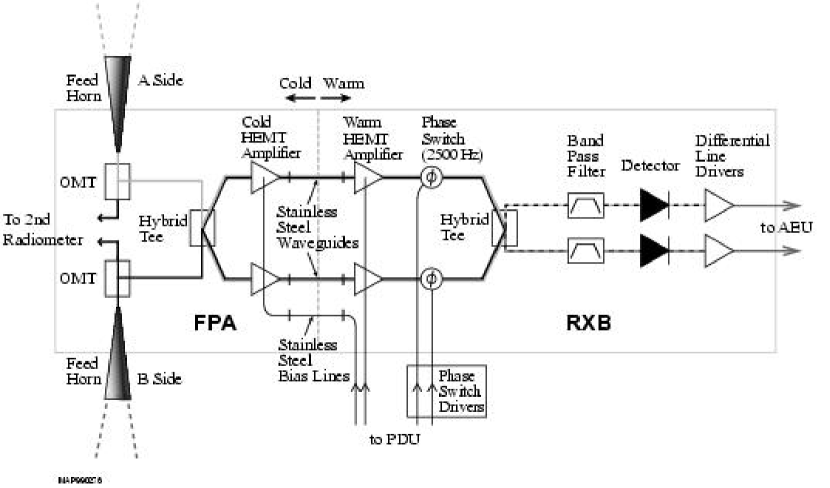
Figure 1: Layout of an individual MAP radiometer. Components on the cold (left) side of the stainless steel waveguides are located in the FPA, and are passively cooled to 90 K in flight.

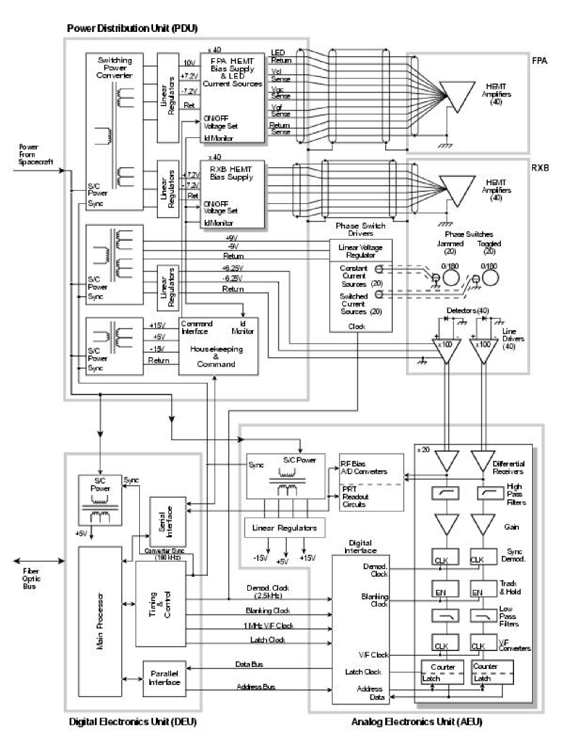
Figure 2: Block diagram of the MAP instrument electronics. The PDU, AEU and DEU boxes are located on the main structure of the spacecraft, and are shaded from direct solar illumination by the shielding provided by the solar arrays. The RXB is located near the center of the spacecraft to provide a stable thermal environment. Microwave interconnections of the radiometer components are shown in Figure 1.

2.2 Nomenclature

Figure 1 is a diagram of the MAP radiometers. The Focal Plane Assembly (FPA) consists of the feed horns, cold portions of the radiometers, and structure, all of which operate near 90 K in flight. The Receiver Box (RXB), which comprises the warm radiometer components, phase switch driver circuit boards, and structure, is located near the center of the satellite and operates at a nominal temperature of $\approx 285$ K. Microwave signals from the FPA are passed to the RXB by 40 thin-wall stainless steel waveguides that provide thermal isolation.

The decision to split the radiometer into warm and cold sections in this manner was motivated by performance, scheduling and cost considerations. Running as few components cold as possible increased reliability by reducing the number of components undergoing large (100 K $-$ 300 K) thermal cycles, saved time by allowing most of the component characterization tests to be performed near room temperature, and eliminated the need for development of cryogenic detectors and preamplifier circuits. The use of warm HEMT amplification stages has performance advantages since $f_{\mathrm{amp}}$ of HEMT amplifiers operating warm is significantly lower than for amplifiers operating cryogenically. This configuration also allowed for an RF tight enclosure to be built around the RXB components, preventing the high level RF signals present in these components from coupling back to the low signal level FPA section, reducing the possibility of ring-type oscillations or other artifacts associated with such feedback. The interior of the RXB and FPA enclosures are lined with microwave absorbing fabric  to dampen cavity modes present in the enclosure.

Radiometers are identified by a three part designator. The first part consists of one or two letters (K, Ka, Q, V or W) that specify the nominal operating frequency band of the radiometer. The second part consists of a single digit $(1-4)$ that indicates which pair of focal plane feed horns are associated with the radiometer. The final part also consists of a single digit (1 or 2) and is used to denote which of the two linear polarizations of the designated feed horn pair the radiometer senses. Designations of ‘$1$’ and ‘$2$’ indicate that the radiometers are connected to the main-arm and side-arm of the orthomode transducers (OMTs) respectively. See Page (2003) for details of the focal plane geometry and polarization orientations of each OMT with respect to the satellite. A pair of radiometers associated with the two polarizations of a given feed is termed a Differencing Assembly (DA) and is specified using only the first two elements of the designator, such as Ka1.

A diagram of the MAP instrument electronics is given in Figure 2. The Analog Electronics Unit (AEU) contains the the data collection circuitry for the radiometers, and the precision readout circuitry for the platinum resistance thermometers. These thermometers monitor the temperature of numerous radiometer components to assist in determining levels of possible systematic errors. The Power Distribution Unit (PDU) contains the DC-DC converters that convert the 31.5 V nominal spacecraft bus voltage to that required by the phase switch drivers, line drivers, and the commandable power supplies which power the FPA and RXB HEMT amplifiers. The Digital Electronics Unit (DEU) contains the digital multiplexers and control circuitry needed to accumulate the science and housekeeping data and pass it to the main computer processor over the spacecraft 1773 fiber optic data bus. The AEU, PDU and DEU are mounted on the outside of the hex hub of the spacecraft structure, are continuously shielded from the Sun by the solar array and are cooled by direct radiation to space. More detailed descriptions of relevant parts these systems are presented later and in Bennett et al. (2003).

2.3 Basic Design

Figure 3 contains a slightly simplified version of the radiometer diagram along with the relevant values of signals present in various sections of the radiometer. ‘A’ and ‘B’ represent the instantaneous, time dependent voltages emitted by cryogenic input loads, Load-A and Load-B, respectively. These loads represent the thermal signal from one linear polarization of the microwave background radiation. In the satellite, these signals are obtained from the output of the OMT attached to the back of the feed horns.

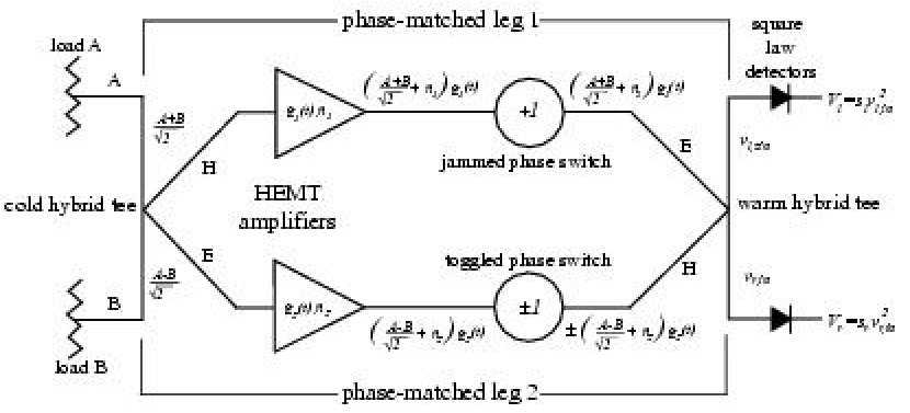
Figure 3: Simplified radiometer diagram used in the description of radiometer operation. The amplifiers’ voltage gain and additive noise voltages are given by $g_{1,2}(t)$ and $n_{1,2}$. The arms of the hybrid tees are labeled E and H. Expressions for signal levels are for voltages.

For simplicity it is first assumed that most of the components in the radiometer are ideal, apart from the amplifiers which are described by instantaneous input referenced noise voltages, $n_{i}$, and instantaneous voltage gains, $g_{i}(t)$, where the index $i=1,2$ specifies in which phase-matched leg the components resides. The time dependent gain of the HEMT amplifiers has been shown explicitly to emphasize that it is not constant, as is usually assumed. It is assumed that all the components between the cold hybrid tees and warm hybrid tees are perfectly phase-matched, so only terms involving intentional differential phase shifts between the legs are presented. The effects of the various non-idealities are discussed in subsequent sections.

Since the signals ‘A’ and ‘B’ are thermally induced noise voltages from two separate loads they are uncorrelated, and hence obey the relations

$$\overline{A} = \overline{B}=0$$ (4)

$$\overline{AB} = 0$$ (5)

$$\overline{AA} \propto k_{B}\Delta\nu T_{a}$$ (6)

$$\overline{BB} \propto k_{B}\Delta\nu T_{b}$$ (7)

where $k_{B}$ is Boltzmann’s constant, $\Delta\nu$ is the bandwidth over which the voltages A and B are measured and $T_{a}$ and $T_{b}$ are the physical temperature of the loads in Kelvin. The over-bar indicates a time average with a period long compared to the period of the microwave signal, but short compared to the time scale of instabilities in any of the microwave components. Given these assumptions, the voltages present at the inputs of the two HEMT amplifiers are

$$\frac{A+B}{\sqrt{2}}\ \textrm{and}\ \frac{A-B}{\sqrt{2}}$$ (8)

where the difference in sign of the B signal reflects the $180^{\circ}$ relative phase shift between the signals in the phase-matched leg introduced by the cold hybrid tee. The signals after amplification by the HEMT amplifiers become

$$u_{1}=\left(\frac{A+B}{\sqrt{2}}+n_{1}\right)g_{1}(t)$$ (9)

$$u_{2}=\left(\frac{A-B}{\sqrt{2}}+n_{2}\right)g_{2}(t)$$ (10)

where $n_{1}$ and $n_{2}$ are the input referenced noise voltages added by the cryogenic HEMT amplifiers.

The phase switches are used to introduce additional 0 or 180^∘ phase shifts between the phase-matched legs. To accomplish this one of them is left ‘jammed’ in one state (here chosen as leg 1) to provide the correct insertion phase while the other (leg 2) is switched between two states. The signals at the output of the warm hybrid tee are then

$$v_{l,\mathrm{in}} = \frac{1}{\sqrt{2}}\left(\frac{A+B}{\sqrt{2}}+n_{1}\right)g_{1}(t)$$ (11)

$$\mbox{}\pm\frac{1}{\sqrt{2}}\left(\frac{A-B}{\sqrt{2}}+n_{2}\right)g_{2}(t)$$

and

$$v_{r,\mathrm{in}} = \frac{1}{\sqrt{2}}\left(\frac{A+B}{\sqrt{2}}+n_{1}\right)g_{1}(t)$$ (12)

$$\mbox{}\mp\frac{1}{\sqrt{2}}\left(\frac{A-B}{\sqrt{2}}+n_{2}\right)g_{2}(t)$$

where the upper sign refers to the signal with the phase switch in the $0^{\circ}$ relative phase state and the lower sign to the switch in the $180^{\circ}$ state. The detectors are operated in the square law region where their output voltage is proportional to the square of their input voltage. The response of these are represented as

$$V_{l}=s_{l}v_{l,\mathrm{in}}^{2}\ \textrm{and}\ V_{r}=s_{r}v_{r,\mathrm{in}}^{2}$$ (13)

for the left and right detectors where $s_{l}$ and $s_{r}$ are the responsivities of the two detectors. In general these responsivities are a function of the input microwave frequency, but for now will be assumed frequency independent and equal so that $s_{l}=s_{r}=s$. The outputs of the two detectors then become

$$V_{l} = \frac{s}{2}\ \biggl{\{}\left(\frac{A^{2}+B^{2}}{2}+n_{1}^{2}\right)g_{1}^{2}(t)$$ (14)

$$\mbox{}+\left(\frac{A^{2}+B^{2}}{2}+n_{2}^{2}\right)g_{2}^{2}(t)$$

$$\mp(A^{2}-B^{2})g_{1}(t)g_{2}(t)\biggr{\}}$$

and

$$V_{r} = \frac{s}{2}\ \biggl{\{}\left((\frac{A^{2}+B^{2}}{2}+n_{1}^{2}\right)g_{1}^{2}(t)$$ (15)

$$\mbox{}+\left(\frac{A^{2}+B^{2}}{2}+n_{2}^{2}\right)g_{2}^{2}(t)$$

$$\pm(A^{2}-B^{2})g_{1}(t)g_{2}(t)\biggr{\}}$$

where equations 4 and 5 have been used together with the fact that the intrinsic voltage noise of the HEMT amplifiers is uncorrelated to the signals from either of the loads, i.e.

$$\overline{n_{i}A}=\overline{n_{i}B}=0.$$ (16)

The outputs consist of three terms. The first two terms arise from the sum of the mean power of the radiometer inputs signals, $\frac{A^{2}+B^{2}}{2}$, and the noise power added by the cryogenic HEMT amplifiers, $n_{i}^{2}$. The contribution arising from the radiometer input signal is proportional to the antenna temperature of the input signals, while the term from the HEMT amplifier’s noise is proportional to the HEMT amplifier’s input-referenced noise temperature. These amplifier noise temperatures range from 30 K $-$ 96 K for K-band through W-band respectively. Both these terms are multiplied by the time dependent gain terms $g_{i}^{2}(t)$, and as such fluctuate due to small gain variations of the amplifiers. Because of the large system bandwidth, even small gain variations can substantially impact the performance of the radiometers. For example, at W-band the nominal effective radiometric bandwidth is $\Delta\nu_{\mathrm{eff}}=19$ GHz, so the fractional change in gain that produces a signal equal to the intrinsic radiometric noise after integrating for one second is,

$$\frac{\Delta g}{g}=1/\sqrt{\Delta\nu\tau}=7.3\times 10^{-6}.$$ (17)

The signal of interest is the third term, which is the difference between the antenna temperatures of the two radiometer inputs, and is multiplied by the product of the voltage gains of the two amplifiers. The magnitude of the prefactor ${(A^{2}-B^{2})}$ is much smaller that that of the first two terms, typically in the mK regime.

There are two techniques for recovering this signal in the presence of the signals from the first two terms, which dominate the detector outputs. The first is to notice that the first two terms appear identically on the output of both detectors whereas the signal of interest appears with the opposite sign on the two detectors. If the output of the detectors are differenced, the offending terms cancel and the desired terms add. This assumes that the responsivities of the two detectors are identical. The other method is to difference the output of each detector with the phase switch in opposite states. In this case the first two terms remain constant and hence cancel, while the third term changes sign when the phase switch flips, and therefore produces a net output. For this method to work the time scale at which the phase switch is switched and the differencing occurs must be short compared to the time scale of the instabilities in the radiometer components, otherwise the value of the first two terms will change in the interim and therefore will not cancel.

The MAP radiometers utilize both techniques. The phase switches are toggled at 2.5 kHz and on board lock-in amplifiers perform the synchronous differencing of each detector’s output. The output of the lock-in associated with each detector’s output is then averaged and telemetered to the ground where the differencing between pairs of detectors is performed. This combination provides optimal rejection of various instabilities. For example, if only the detector - detector differencing were performed low frequency drifts in the detector responsivity and offset voltage drifts of the following video amplifiers would limit the performance of the radiometer. On the other hand if only the temporal differencing were performed the switching frequency of the phase switches would have had to be substantially increased due to the proximity of the $1/f$ knee of the W-band amplifiers. This would have increased the ‘dead time’ of the detectors due to the blanking interval and hence reduced the sensitivity of the radiometers. (See Section 5.3.)

Figure 4 presents a noise power spectral density measurement of the W11 radiometer made during the radiometer assembly and testing program. Demodulated data for each detector, L and R, and the normalized mean, $(\mathrm{L}+\mathrm{R})/2$ and difference $(\mathrm{L}-\mathrm{R})/2$ of the detector signals are displayed. The noise power spectral densities are flat to very low frequencies as expected, despite the fact that the amplifiers’ $f_{\mathrm{knee}}$ frequency for the RF bandwidth of this radiometer is $\approx 1$ kHz. In the absence of gain fluctuations, the difference signal between the detectors should have a noise power level lower by a factor of $\sqrt{2}$ than each detector’s individual noise. Note that the noise power spectral density of the difference signals is lower that the individual detector noises by more than this factor. This occurs because there is still a substantial degree of amplifier gain fluctuations present at the 2.5 kHz phase switch drive frequency. This contributes additional correlated noise to both detectors, in addition to the intrinsic radiometer noise. When the detector signals are differenced this additional correlated term cancels, as described above, resulting in a noise power reduction of greater than $\sqrt{2}$ relative to the individual detector noises.

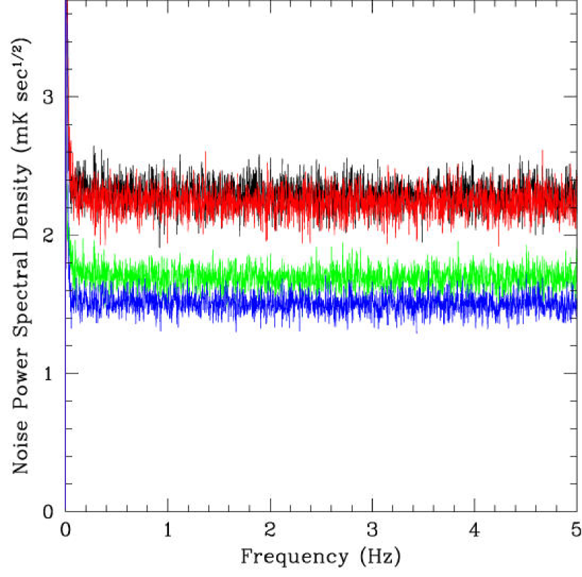
Figure 4: Power Spectral Density of the MAP W11 radiometer. The red and black traces are the power spectral density measurements of the two detectors on the radiometer. The green and blue traces are the spectral densities of the normalized sum and difference of the detector signals. During these measurements the FPA HEMT amplifiers were operating at a physical temperature of $\approx 75$ K and the loads attached to the inputs of the radiometer were regulated to 25 K.

2.4 Departures From Ideality

Non-idealities in the components comprising the radiometers lead to effects not described by the previous analysis. A detailed model simultaneously incorporating all such effects would prove complicated and not readily understandable. Instead, the largest and most important effects are described individually so as to provide an understanding of how each term relates to the overall radiometer performance. In doing so, it is important to realize that the radiometers’ ‘signal’ and ‘noise’ are often altered differently by these effects.

2.4.1 Chain to Chain Amplitude and Phase Match

Since the switching is accomplished through phase modulation, it is important to understand how phase and amplitude mismatches between the two phase-matched legs affect radiometer performance. There are two types of phase error that can occur. Nominally there should be a $180^{\circ}$ difference in the insertion phase of the phase switch between its two states. Fortunately the phase switches are excellent in this respect, with departures from ideality of $<3^{\circ}$. Such small errors do not significantly affect the radiometers’ performance. The more important phase error is the departure from the $0^{\circ}$ (or $180^{\circ}$) phase match between the two legs of the radiometer. These errors are typically much larger since each leg comprises several components, each of which can contribute to the mismatch.

First consider effects on the signal terms. Equation 11 describes the input voltage to one of the square law detectors. Ideally $g_{1}(t)=g_{2}(t)=g$, so signals originating from source A travel through both legs of the radiometer and appear at the input of the square law detector with equal amplitude and the same (or opposite) phase so that that they add (or cancel). The signal at the output of the square law detector from source A therefore is either $\frac{s}{2}(A^{2}g^{2})$ or $0$, depending on the phase switch state. In the presence of phase and amplitude mismatches the voltage signals at the input of the detectors for the two phase switch states become $\frac{1}{2}A(g_{1}(t)+g_{2}(t))$ and $\frac{1}{2}A(g_{1}(t)-g_{2}(t))$. After square law detection and demodulation the resulting signal is $\frac{s}{2}A^{2}g_{1}(t)g_{2}(t)\cos(\theta)$, where $\theta$ is the phase error as shown in Figure 5. Signals from the ‘B’ source are affected similarly, so the net effect is that the amplitudes of the modulated signals output from each detector, $S_{i}$, are

$$S_{l}\propto-s_{l}(A^{2}-B^{2})g_{1}(t)g_{2}(t)\cos(\theta)$$ (18)

$$S_{r}\propto+s_{r}(A^{2}-B^{2})g_{1}(t)g_{2}(t)\cos(\theta).$$ (19)

Figure 5: Vector diagram showing the relative phase angle of the amplified voltage signals from source A for both phase switch states. The relative phase shift between the phase-matched legs is $\theta$.

The noise is affected quite differently. The noise in the two phase-matched legs of the radiometer is uncorrelated since it originates from different amplifiers. The noise voltages present at the input of the left and right detectors are $\frac{u_{1}+u_{2}}{\sqrt{2}}$ and $\frac{u_{1}-u_{2}}{\sqrt{2}}$, where $u_{1}$ and $u_{2}$ are defined by Equations 9 and  10. The corresponding instantaneous input powers to the detectors are $\frac{(u_{1}+u_{2})^{2}}{2}$ and $\frac{(u_{1}-u_{2})^{2}}{2}$, while average power on both detectors is the same and is given by $\frac{\overline{u_{1}^{2}}+\overline{u_{2}^{2}}}{2}$. The detectors operate in the square law region, so the instantaneous and mean detector voltages are

$$V_{l}=\frac{s_{l}}{2}(u_{1}+u_{2})^{2}, \overline{V_{l}}=\frac{s_{l}}{2}(\overline{u_{1}^{2}}+\overline{u_{2}^{2}})$$ (20)

$$V_{r}=\frac{s_{r}}{2}(u_{1}-u_{2})^{2}, \overline{V_{r}}=\frac{s_{r}}{2}(\overline{u_{1}^{2}}+\overline{u_{2}^{2}}).$$ (21)

The variances of the detector output voltages, $N_{i}^{2}$ — measures of the radiometer noise — are proportional to the square of the total power incident on each detector and are given by

$$N_{l}^{2}=\overline{V_{l}^{2}-\overline{V_{l}}^{2}}=\overline{V_{l}^{2}}-\overline{V_{l}}^{2}=\frac{s_{l}^{2}}{2}(\overline{u_{1}^{2}}+\overline{u_{2}^{2}})^{2}$$ (22)

$$N_{r}^{2}=\overline{V_{r}^{2}-\overline{V_{r}}^{2}}=\overline{V_{r}^{2}}-\overline{V_{r}}^{2}=\frac{s_{r}^{2}}{2}(\overline{u_{1}^{2}}+\overline{u_{2}^{2}})^{2}.$$ (23)

The variance of the difference between the detector voltages, $N_{\mathrm{diff}}^{2}$, is

$$N_{\mathrm{diff}}^{2} = \overline{(V_{l}-V_{r})^{2}}-\overline{(V_{l}-V_{r})}^{2}$$ (25)

$$= (\overline{V_{l}^{2}}-\overline{V_{l}}^{2})+(\overline{V_{r}^{2}}-\overline{V_{r}}^{2})$$

$$\mbox{}-2\overline{(V_{l}-\overline{V_{l}})(V_{r}-\overline{V_{r}})}$$

$$= s^{2}(\overline{u_{1}^{2}}+\overline{u_{2}^{2}})^{2}-s^{2}(\overline{u_{1}^{2}}-\overline{u_{2}^{2}})^{2}$$ (26)

$$= 4s^{2}\overline{u_{1}^{2}}\ \overline{u_{2}^{2}}$$ (27)

where the relation

$$\overline{(V_{l}-\overline{V_{l}})(V_{r}-\overline{V_{r}})}=\frac{s^{2}}{2}(\overline{u_{1}^{2}}-\overline{u_{2}^{2}})^{2}$$ (28)

has been used to relate the covariance of the detector output voltages to the power incident to the two inputs of the warm hybrid tee as shown in Appendix A. It has also been assumed that the responsivity of the two detectors are identical, $s_{l}=s_{r}=s$. This is achieved in practice by separately telemetering the signals from the two detectors to the ground and individually calibrating them before calculating the difference.

It is a good approximation to assume that the input referenced noise temperature of the two amplification chains within a radiometer are equal, $n_{1}=n_{2}$. The signal to noise ratio, $\frac{S_{i}}{N_{i}}$, for each detector then depends on the phase and gain mismatch between the phase-matched legs, (Equations 18, 19, 22, 23)

$$\frac{S_{i}}{N_{i}}\propto\frac{\overline{g_{1}}\ \overline{g_{2}}\cos(\theta)}{\sqrt{\overline{g_{1}^{2}}+\overline{g_{2}^{2}}}},$$ (29)

however, the signal to noise ratio for the difference of the detector outputs is independent of the gain mismatch, (Equations 18, 19, 27 )

$$\frac{S_{r}-S_{l}}{N_{\mathrm{diff}}}\propto\cos(\theta).$$ (30)

This behavior is similar to that of a true correlation radiometer, and results from the existence of the detector noise covariance as described in Appendix A.

The covariance between the output of the two detectors (Equation 28) of each radiometer was used as a diagnostic to verify the health of the radiometers during integration and testing. Any change from the nominal value measured during radiometer assembly would indicate a change in the relative RF gain of the amplification chains. Similar data are available during flight, since the two detector outputs are separately telemetered to the ground and provides a continuous monitor of the gain balance between the two phase-matched legs of each radiometer.

The MAP design specification was to hold the gain imbalance between chains to $\pm 2$ dB and the phase difference to $\pm 20^{\circ}$, making the loss in sensitivity from the phase error $<$ 6%. It should be noted that although the above relation describes the independence of the signal to noise ratio from amplifier gain imbalances, any other sources of gain mismatch, due to imbalances in the hybrid tees or losses in the waveguides or phase switches affect the signal to noise ratio in the exact same way, so the gains in the previous equations can be thought of as the gain of the entire system between the hybrid tees.

2.4.2 Crosstalk in the Cold Hybrid Tee

Imperfect isolation between the two ports of the cold hybrid tee connected to the cryogenic HEMT amplifiers is a potential source of a radiometric offset. Consider the noise voltage, $n_{1}$, emitted from the input of one of the cryogenic HEMT amplifiers. The magnitude of this voltage will roughly correspond to the input referenced noise temperature of the HEMT amplifier. This noise will have some correlation with the output voltage of the HEMT amplifier (Wedge, 1992). Let the correlation coefficient between these voltages be $\beta$. Although the value of this coefficient is not well known, it is expected to fall in the range of 0.1 to 0.3. If the power isolation between the E and H ports of the hybrid tee is $\alpha$, the resulting voltage at the input of the other cryogenic HEMT amplifier produced by the noise voltage output from the first will be

$$v_{\mathrm{in2}}=n_{1}\sqrt{\alpha}$$ (31)

where typical values of $\alpha$ are $\approx 1\times 10^{-4}.$ Since this signal is coherent between the two phase-matched legs of the radiometer, it can produce an additional contribution to the total detector power that is modulated by the phase switch. The size of this effect will be roughly

$$T_{\mathrm{off}}\approx(n_{1}^{2}+n_{2}^{2})\beta\gamma\sqrt{\alpha}$$ (32)

where $\gamma$ is an additional factor that allows for the effect of bandwidth averaging. Its magnitude is roughly $\gamma\approx l_{c}/\Delta l$ for $\Delta l>l_{c}$, where $l_{c}\approx c/\Delta\nu_{\mathrm{eff}}$ is the coherence length of the microwave signal, determined by the bandwidth of the radiometer, $\Delta\nu_{\mathrm{eff}}$, and $\Delta l\approx 5\mbox{$\textrm{cm}$}$ is the path length difference between the two paths the signals travel before being recombined in the warm hybrid tee. Since noise emitted from both amplifiers contributes to this effect, its magnitude is proportional to the sum of the noise temperatures. The desire to minimize the size of this effect led to the configuration in which the amplifiers are attached to the E and H arms of the hybrid tees, since the E-H arm isolation is typically 10 dB better than the colinear-colinear arm isolation.

There is an additional term that can also contribute to this effect caused by reflections from either the OMT or the corrugated feed. In this case the power emitted from the input of the HEMT amplifier enters the cold hybrid tee through an E or H-port and is coupled to the colinear ports. This signal is then reflected from the OMT or feed horn, re-enters the cold hybrid through the colinear ports and is coupled to the opposite H or E-port. This effectively reduces the E-port to H-port isolation of the cold hybrid tee. The contribution from this effect to a radiometer’s offset is $\approx 0.2$ K.

2.4.3 Toggled Phase Switch Transmission Imbalance

Slight differences between the frequency dependence of the toggled phase switch’s transmission coefficients in its two states can lead to an effective radiometer offset. This occurs if the frequency responses of the two detector/filter combinations on a radiometer differ. The detector output voltage for detector $j$ with the phase switch in state $i$ can be expressed as

$$V_{i,j}=\int u^{2}(\nu)t_{i}(\nu)s_{j}(\nu)d\nu+V_{j}^{0}$$ (33)

where $u^{2}(\nu)$ is the RF noise power spectral density entering the toggled phase switch, $t_{i}(\nu)$ is the frequency dependent power transmission coefficient of the phase switch in the two states, $i=1,2$, and $s_{j}(\nu)$ is the frequency dependent responsivity of the detector filter combination, $j=L,R$. The integral extends over the RF bandwidth of the radiometer, and $V_{j}^{0}$ is a constant detector output voltage arising from the noise power from the unswitched leg of the radiometer.

Consider the situation where all other sources of radiometric offset vanish. The condition to null the modulated component of the right detector output voltage is $V_{1,R}=V_{2,R}$, however this does not ensure that the modulated component of the left detector’s output voltage will vanish, $V_{1,L}=V_{2,L}$, unless $s_{L}(\nu)=s_{R}(\nu)$. In fact, it raises the question as to the definition of the offset for this type of radiometer. The definition used by MAP is that a radiometer’s offset is the temperature difference between thermal loads connected to the radiometer’s inputs that produces the condition $V_{1,R}-V_{2,R}=V_{1,L}-V_{2,L}$. Once this condition is achieved by setting the temperature of the test input loads, the difference between the average losses of the two states of toggled phase switch is adjusted to make both $V_{1,R}-V_{2,R}=V_{1,L}-V_{2,L}=0$ by adjusting the phase switch bias currents. This definition of offset has the advantage that it is independent of the sign and gain of the data collection system used to record the detector output voltages.

2.4.4 Standing Waves

Standing waves between the cold and warm HEMT amplifiers degrade the phase match and gain flatness of the radiometers, with the associated reductions in sensitivity previously described. Traditionally, isolators are used to eliminate standing waves, however the only viable isolator for MAP radiometers, given the large fractional bandwidths, would be Faraday rotation isolators. Such isolators unfortunately exhibit small changes in characteristics under the influence of externally applied magnetic fields. The Cosmic Background Explorer (COBE) used isolators (Kogut et al., 1996), as well as ferrite switches, and needed to correct the data for variations resulting from the changing orientation of Earth’s magnetic fields with respect to the spacecraft, even though efforts were made to magnetically shield the ferrite devices. Despite the fact that MAP operates far from Earth, and therefore in a much smaller magnetic field, $\approx 100$ nT, there were still concerns related to magnetic fields generated on board the spacecraft from the reaction wheels and other high current spacecraft systems.

For the higher frequency bands the loss in the phase-matched waveguides is sufficient to reduce the standing waves to acceptable levels. For example, at W-band the loss in the phase-matched waveguides is approximately 6 dB, so the largest amplitude and phase variations resulting from standing waves are approximately $\pm 2.2$ dB and $\pm 14^{\circ}$ respectively, even if the inputs of the warm amplifiers and outputs of the cold amplifiers had 0 dB return losses. With typical input and output return losses of 4 dB and 10 dB these variations in amplitude and phase are approximately $\pm 0.4$ dB and $\pm 3^{\circ}$. At lower frequencies the loss in the interconnecting waveguide is much smaller, typically 1 dB. When combined with the typical input and output return losses of the amplifiers of about 8 dB, the amplitude and phase variations are approximately $\pm 1.2$ dB and $\pm 8^{\circ}$. For all frequency bands the performance degradation resulting from these effect was small enough that no isolators were used.

Standing waves between the outputs of the RXB amplifiers and the detectors are also of concern. Not only do they introduce gain flatness errors and phase errors as previously described, but, since the toggling phase switch modulates these standing waves, they can introduce an effective offset into the radiometer if the frequency responses of the two filter/detector combinations on a radiometer are not identical. This effect is similar to that resulting from the transmission mismatch of the phase switch, but in this case the spectrum of the available noise power, determined by the standing wave mode pattern, is modulated by the state of the phase switch. This effect was minimized by using detectors with input matching circuits that reduced their reflection coefficients.

3 Systematic Errors

Potential sources of radiometer induced signals contributing to the systematic error budget included random output drifts as well as terms arising from temperature and power supply fluctuations, varying magnetic fields, either external or internal to the spacecraft, microphonics, and particle hits. The MAP radiometer systematic error analysis categorized errors into two types, additive and multiplicative. Additive signals are those that add linearly to the radiometer output signals, such as varying emission from the optics or feeds. Multiplicative signals are those that modulate the effective gain of the radiometer and therefore require a non-zero radiometer output to have affect. In practice the only significant multiplicative terms are those arising from the product of small radiometer gain fluctuations and the radiometers’ offsets. For the purpose of estimating the size of these terms, offsets were assumed to be 1 K for all radiometers. Spin synchronous effects arise when some driving function coupled to the spacecraft orientation, such as a temperature or power supply voltage, induces a change in the output of a radiometer by varying the characteristics of one or more of its components.

During development the magnitudes of the estimated systematic errors were calculated based on current estimates of the maximum size of the expected driving functions for each component. The driving functions were multiplied by susceptibility coefficients relating how each ultimately perturbed the output of the radiometers through either additive or multiplicative terms. The susceptibility coefficients were derived by measuring the variation of important component parameters as a function of the driving parameters. It was often necessary to vary the driving parameter over a much larger range than expected in flight in order to measure a susceptibility coefficient. In such cases it was assumed that the component’s response scaled linearly with the driving function. The radiometer model was used to calculate the resulting perturbations of the radiometer’s outputs. Given the symmetric design of the observatory, and the long thermal time constants relative to the spin period of the spacecraft, it was assumed that the various systematic error terms have random phases relative to one another, so systematic error contributions were added in quadrature. For the purpose of design, the spin synchronous temperature variation of the FPA and RXB components was assumed to be 0.5 mK peak, and the spin-synchronous temperature fluctuations of the AEU, DEU and PDU components was assumed to be 10 mK peak. Table 2 summarizes the radiometer related systematic error terms identified. This analysis was used to evaluate trade offs and tests used throughout the development process, but does not necessarily reflect the amplitude of the effects in flight data.

Table 2: Systematic Error Terms

Component	Susceptibility $\times$ Forcing function	Effect
Feed horns	$\epsilon\times\Delta(T_{a}-T_{b})$	A
Orthomode transducer	$\epsilon\times\Delta(T_{a}-T_{b})$	A
OMT - hybrid waveguides	$\epsilon\times\Delta(T_{a}-T_{b})$	A
FPA hybrid tee	$(\epsilon_{a}-\epsilon_{b})\times\Delta T$	A
FPA HEMT amplifiers	$dg/dx\times\{\Delta V_{\mathrm{gc}},\Delta V_{\mathrm{gf}},\Delta V_{d},\Delta T,\Delta I_{\mathrm{LED}}\}$	M
RXB HEMT amplifiers	$dg/dx\times\{\Delta V_{\mathrm{gf}},\Delta V_{d},\Delta T$ }	M
Band definition filters	$dS_{21}/dt\times\Delta T$	$A^{*}$,M
Phase switches	$d(S_{21}(0^{\circ})-S_{21}(180^{\circ})/dx\times\{\Delta T,\Delta I$}	$A^{*}$,M
Detectors	$ds/dT\times\Delta T$	M
Line drivers	$dg/dx\times\{\Delta V_{\mathrm{dd}},\Delta V_{\mathrm{ss}},\Delta T$ }	M
AEU	$\{dA_{v}/dx,dO_{v}/dx\}\times\{\Delta T,\Delta V_{\mathrm{bus}}\}$	A, M
PDU	$\{dV_{\mathrm{gc}}/dx,dV_{\mathrm{gf}}/dx,dV_{d}/dx,dI_{\mathrm{LED}}/dx\}\times\{\Delta T,\Delta V_{\mathrm{bus}}$ }

The forms of systematic error terms incorporated into the model used to estimate the size of artifacts on the radiometers’ outputs. The first column lists the component originating the effect. The second column contains the relation describing the component’s varying performance characteristic in the form coefficient $\times$ forcing function. The coefficient is either a fixed parameter such as an emissivity, $\epsilon$, or the derivative of a parameter, $d/dx$, with respect to a forcing function $x$. For the AEU $A$ and $O$ represent the gain and offset of the entire data collection system from the line driver inputs to the digitized outputs. For the PDU and HEMT amplifiers $V_{\mathrm{gc}}$, $V_{\mathrm{gf}}$, and $V_{d}$ refer to the gate and drain power supply voltages and $I_{\mathrm{LED}}$ the LED current supplies as described in Sections  4.1 and 5.1.1. For the filters and phase switches $S_{21}$ is the forward transmission element of the scattering matrix. The forcing function describes which external variable changes to induce the effect. Temperatures of the component in the first column are indicated by $T$. For the phase switches $I$ refers to the PIN diode drive current. The line driver power supply voltages are $V_{\mathrm{dd}}$ and $V_{\mathrm{s}}$, and $V_{\mathrm{bus}}$ refers to the voltage of main spacecraft power. Subscripts ‘$a$’ and ‘$b$’ refer to items associated with the different focal planes. When more than one parameter or forcing function is important they are enclosed by braces. The final column indicates the form of the perturbing term, ‘M’ for multiplicative terms and ‘A’ for additive terms. Terms marked $A^{*}$ are additive terms that effect both detectors of a radiometer in common mode, and so should cancel when the detector outputs are differenced as the data is processed. It was estimated that 10 % of the effect could survive the differencing, so that was the proportion of the effect included in the error analysis. Variation in the PDU’s performance produces driving functions that are used as inputs to other terms.

During radiometer assembly and testing, the overall radiometer susceptibility to varying temperature, power supply voltage, and magnetic fields was measured to ensure that the actual radiometer susceptibilities met specification. These susceptibility coefficients were remeasured after the 10 DAs were integrated into the instrument structure in a series of tests performed in thermal-vacuum chambers at Goddard Space Flight Center (GSFC). Tests were performed both before and after an instrument level vibration, and results were compared to ensure that no significant changes in the radiometers’ performance occurred as a result of the vibrations. During these tests the radiometers were operated by the flight electronics and in an environment close to that expected in flight. The radiometers’ inputs were attached to the flight feed horns, each of which had a full aperture temperature regulated cryogenic load attached to its open end to mimic the microwave background radiation signal. Following the integration of the instrument to the spacecraft another set of thermal vacuum tests was performed in the Space Environment Simulator to search for signals induced in the radiometers from interactions with spacecraft systems.

The data obtained during all the aforementioned tests were used to calculate approximate susceptibility coefficients. Measurements were also performed during the thermal vacuum tests to measure the size of the driving functions expected in flight. These data, in combination with the in-flight measurements of numerous temperatures, voltages and currents in the radiometer system, will be used to estimate and/or limit the magnitude of systematic error signals produced in flight. The results of the instrument level and spacecraft level tests indicate that the MAP radiometers will meet their systematic error requirements in-flight without applying any corrections to the radiometric data.

4 Components

The MAP radiometers are built from numerous discrete components, with little integration of multiple functions within a component. This approach eliminated the design time associated with custom components, allowed for simple characterization and testing of each component, and for the selection and matching of component characteristics when required. It also increased the number of potential suppliers for components since the number of suppliers of highly integrated components is very limited.

Most of the microwave components were of standard commercial quality, with GSFC providing quality assurance oversight, including materials analysis and qualification testing. Microwave joints were wrapped with flexible microwave absorber  wherever possible to block potential leakage. Important performance characteristics of the major components of the MAP radiometers are provided in the following sections.

4.1 HEMT Amplifiers

The HEMT amplifiers at the heart of the radiometers were designed, fabricated and tested at the National Radio Astronomy Observatory (NRAO) Central Development Laboratory (Pospieszalski, 2000). The HEMT devices were manufactured by Hughes Research Laboratories. Key amplifier performance parameters, summarized in Table 3, include noise temperature, gain flatness, RF bandwidth and power dissipation.

Table 3: Flight Radiometer HEMT Amplifier Specifications

Frequency range (GHz)	20-25	28-37	35-46	53-69	82-106
Noise temperature @85 K (K)	$30\pm 2$	$33\pm 3$	$48\pm 5$	$64\pm 7$	$96\pm 7$
Noise temperature @300 K (K)	$\approx 100$	$\approx 115$	$\approx 150$	$\approx 260$	$\approx 370$
Gain (@85 K/@300 K) (dB)	34/33	34/32	34/31	35/31	35/32
Gain flatness (dB)	$\pm 1.5$	$\pm 1.0$	$\pm 1.5$	$\pm 2.5$	$\pm 3$
# gain stages	4	4	4	5	6
Dissipation(RXB) (mW)	$\approx 40$	$\approx 45$	$\approx 45$	$\approx 45$	$\approx 55$
Dissipation(FPA) (mW)	$\approx 22$	$\approx 30$	$\approx 25$	$\approx 12$	$\approx 25$
Mass (kg)	0 .131	0.121	0.132	0.114	0.116
Phase match (degrees)	$\pm 15$	$\pm 15$	$\pm 20$	$\pm 20$	$\pm 25$

The amplifiers are built using discrete devices, stripline matching elements and wire bonded interconnections. Early in the program NRAO demonstrated the feasibility of building amplifiers at MAP’s highest frequency band with highly reproducible characteristics. Monolithic Microwave Integrated Circuit (MMIC) designs were considered, but rejected based on cost and schedule concerns. The FPA and RXB amplifiers in each frequency band are of identical design. In addition to requiring only one design per band, this also provided for more flexibility in selecting and matching amplifiers in order to optimize radiometer performance.

Each amplifier has one drain voltage supply, $V_{d}$, common to all the transistors with nominal input voltages between +1.000 V and +1.500 V. Two gate bias supplies are provided on each amplifier, one supplies gate bias voltage to the input stage, $V_{\mathrm{gc}}$, the other to all the remaining stages, $V_{\mathrm{gf}}$. This biasing arrangement was chosen to allow for re-biasing the input stage of the cryogenic amplifiers for optimum noise performance, should the need arise. The externally applied gate bias voltages range from 0.0 V to $-0.500$ V. Internal resistive voltage dividers divide this voltage to that required by each device to compensate for variability in transistor characteristics. Since cryogenic operation of HEMTs may require illumination, two light emitting diodes (LEDs) were designed into each amplifier body. The amplifiers installed in the RXB have both gate bias inputs fed by a common voltage supply, since the ability to re-bias the input stage individually is not required, and the LEDs remain unpowered.

4.1.1 Amplifier ‘Burn-in’

During the construction of the first flight radiometers (Q1) it was observed that the drain current for a given gate bias and drain voltage displayed a slow rise when operating at room temperature, with a corresponding rise in amplifier gain. Similar effects are seen with the K, Ka and V band amplifiers, all of which are constructed using HEMT devices from a wafer which has a SiN passivation layer. The W-band amplifiers use HEMT devices from an unpassivated wafer and do not exhibit this effect. The size of the effect is largest for the small geometry devices used in the higher frequency amplifiers, and seems to arise from a thermally activated process. Once the amplifiers are cooled to $\approx 100$ K the ‘burn-in’ ceases. The largest effect is observed in V-band, were the power gain, $g(t)^{2}$, can be described approximately as $g^{2}(t)=g_{0}^{2}(1+\eta(1-e^{-t/\tau}))$ with $\eta\approx 1$ and $\tau\approx 140$ hours. When kept at room temperature and unpowered the amplifier’s gain slowly returns to its initial state with a time constant of $\approx 500$ hours.

During the radiometers’ assembly the amplifiers were powered continuously, so the radiometers were constructed and characterized with the amplifiers fully burned-in. Small changes in the insertion phase of the amplifiers associated with the gain changes, could effect the in-flight radiometer performance. The greatest concern relates to our knowledge of the frequency dependent bandpasses of the radiometers. Such effects are expected to be small, since both amplifiers in a radiometer will always have the same degree of burn-in. However, to ensure proper performance in flight, the radiometers remained powered as much as practicable immediately before launch, since once launched the FPA temperature quickly falls preventing further burn-in of the FPA amplifiers. Measurements are being performed on an engineering model of a V-band radiometer to estimate the additional uncertainty in the knowledge of the radiometers’ bandpasses, but it is not expected to be a significant effect.

4.2 Phase-Matched Waveguides

The phase-matched waveguides connect the output of the cold FPA HEMT amplifiers to the inputs of the warm RXB amplifiers and were fabricated by Custom Microwave Inc. Each waveguide incorporates $\approx 25$ cm straight section of commercially available 0.025 cm wall stainless steel waveguide serving as a thermal break. Copper sections, overlapping $\approx 2.5$ cm at each end, were electro-formed directly onto both ends of each stainless steel section, reducing the effective length of the thermal break to $\approx$ 20 cm. Tellurium-copper waveguide flanges with over-sized exterior dimensions were soldered to the copper ends of each waveguide assembly for transition to other waveguide components and structural support. No plating or passivation treatment was applied to either the copper or stainless steel sections of the waveguides. Insuring a broad-band phase match required careful control of the dispersion relation of the waveguides. Each phase-matched pair was designed to have the same overall length and the same number and radii of ‘E’ and ‘H’ bends. The electro-formed sections were fabricated on precision formed mandrels, that were hand lapped to reduce deformations in their cross section caused by bending. The dimensional tolerances of the commercially available stainless steel waveguide sections were not well enough controlled to ensure a uniform dispersion relation from sample to sample, so each stainless steel section was characterized, and matched sections delivered to Custom Microwave for incorporation into the waveguide assemblies. To allow for manufacturing variations, the radiometer design used waveguide shims, up to one half a guide wavelength, to be inserted at the warm end of one or both of the waveguide assemblies to adjust the electrical length of the assembly.

4.3 Phase Switches

The phase switches use a suspended stripline architecture and were manufactured by Pacific Millimeter Products. They can be set to two states differing in insertion phase by very nearly $180^{\circ}$, largely independent of frequency. Switching is accomplished by forward biasing one of two back-to-back connected PIN diodes  through application of $\approx\pm 20$ mA drive current to the control input. Table 4 summarizes some of the important parameters of these devices. The housings were made of gold plated aluminum, and the RF input and output connections were made with integrated waveguide to stripline transitions. The PIN diode bias was applied using high speed constant current sources, switching polarity at 2.5 kHz. Precision matching of the average insertion loss between the two states was obtained by adjusting the relative magnitudes of the positive and negative bias currents. As the drive current to the PIN diode is reduced, the rate of change of the forward power transmission coefficient with respect to drive current, $\Delta S_{21}/\Delta i$, increases. For the purpose of estimating systematic errors from drive current variations, a conservative value of $\Delta S_{21}/\Delta i=0.03$/mA was used, based on measurements made with a PIN diode drive current of 5 mA.

Table 4: Flight Radiometer Phase Switch Specifications

MAP Band Designation	K	Ka	Q	V	W
Frequency range (GHz)	20-25	28-36	35-46	53-69	82-106
Insertion loss (dB)	$\approx 1.2$	$\approx 1.4$	$\approx 1.4$	$\approx 1.5$	$\approx 2.5$
Loss balance (dB)	$\approx 0.1$	$\approx 0.1$	$\approx 0.1$	$\approx 0.1$	$\approx 0.3$
Phase difference (degrees)	$\pm 2$	$\pm 2$	$\pm 3$	$\pm 3$	$\pm 3$

4.4 Band Definition Filters

The band definition filters also used a suspended stripline technique, and were supplied by Microwave Resources Inc. They were manufactured with unplated aluminum bodies. Filter inputs and outputs are through waveguide ports, again implemented using integrated waveguide to stripline couplers. The band-edge frequencies and roll-off characteristics were specified to limit the bandpass to frequencies where the input OMTs had acceptable return losses. Radiometric response where the OMT reflection coefficient becomes large could lead to large radiometric offsets. Table 5 summarizes the microwave performance specifications of these filters.

Table 5: Flight Radiometer Band Definition Filter Specifications

MAP Band Designation	K	Ka	Q	V	W
$-1$ dB frequency (GHz)	20.0, 25.0	28.5, 36.5	36, 44.5	54.5, 67.5	84, 104
$-15$ dB frequency (GHz)	19.0, 26.0	27.0, 38.0	34, 46.5	51.5, 70.5	80, 108
Passband ripple (dB)	$\pm 0.25$	$\pm 0.25$	$\pm 1$	$\pm 1$	$\pm 1$
Insertion loss (dB)	$\approx 1$	$\approx 1.2$	$\approx 2.4$	$\approx 2$	$\approx 3$

4.5 Hybrid tees

Both the FPA (cold) and RXB (warm) hybrid tees were manufactured by Millitech Corp. The designs are based on Millitech’s CMT series (90% bandwidth version) hybrid tee. Changes made for MAP include using aluminum bodies to reduce the mass, and, to eliminate the possibility of detached flakes, no gold plating. A special epoxy, suitable for cryogenic operations, was used to secure the tuning post, and several screw holes were added and relocated for mounting.

4.6 Cold Hybrid Tee to OMT Waveguides

These are the waveguide sections that connect the output of the OMTs to the inputs of the cryogenic hybrid tees. They were fabricated from standard commercially available drawn copper waveguide and had waveguide flanges hard soldered to their ends. The waveguide sections were bent and flanges attached by Microwave Engineering Corporation. After fabrication they were annealed in a hydrogen atmosphere to remove the work-hardening resulting from the forming process.

4.7 Orthomode Transducers

Orthomode transducers for all 5 frequency bands were designed and manufactured for MAP by Gamma-f Corp. All are made of electro-formed copper and have very low insertions loss (Barnes, 2002). Table 6 summarizes some of the OMTs important performance characteristics. The design of the OMTs limit the usable microwave bandwidth of the radiometers.

Table 6: Flight Radiometer Orthomode Transducer Specifications

MAP Band Designation	K	Ka	Q	V	W
Frequency range (GHz)	$20-25$	$28-36$	$35-46$	$53-69$	$82-106$
Return loss (dB)	$<-15$	$<$-14	$<$-14	$<-15$	$<-14$
Isolation (dB)	$>40$	$>$30	$>$30	$>27$	$>25$
Insertion loss (dB)	$<0.1$	$<0.12$	$<0.13$	$<0.15$	$<0.22$

4.8 Detectors

The MAP detectors were designed and supplied by Millitech Corp. They are a special design and include a tuning element before the detector diode to lower their reflection coefficient, reducing the size of the standing wave between the detector and the output of the RXB HEMT amplifier (Sec 2.4.4). In order to design the line driver circuit it was necessary to measure the detectors’ video output characteristics. For output voltages up to $\approx 10$ mV the detectors have a very nearly square law response and can be modeled as a noiseless voltage source and a series resistor in the $2000-3500~{}\Omega$ range. The resistor determines both the video output impedance of the detector and the Johnson voltage noise if it is assumed to be at $\approx 300$ K physical temperature. Table 7 contains a number of the key performance parameters of the detectors. The responsivity typically decreases with temperature by $\approx 0.01$ dB/K.

Table 7: Flight Radiometer Detector Specifications

MAP Band Designation	K	Ka	Q	V	W
Frequency range (GHz)	$20-25$	$28-36$	$35-46$	$53-69$	$82-106$
Return loss (dB max.)	$-3$	$-5$	$-5$	$-2$	$-3$
Return loss (dB avg.)	$-6$	$-10$	$-6$	$-10$	$-7$
Responsivity (typical V/W)	$3000$	$3500$	$2000$	$2000$	$2000$
Responsivity flatness (dB)	$\pm 2$	$\pm 1.2$	$\pm 1$	$\pm 1.6$	$\pm 2$

4.9 Line Drivers

The line drivers are x100 gain amplifiers built on small circuit boards attached directly to the video output of the detector diodes. They boost the relatively small output voltages from the detector ($\approx 10$ mV) to a high level differential signal, suitable for transmission over the instrument harness to the AEU. The line drivers were designed to limit the increase of the nominal operating detector output noise by $<0.5\%$, and have enough dynamic range to ensure operation at room temperature (necessary during integration and testing) without saturation. The input stage of the line driver is an Analog Devices AD524 instrumentation amplifier. A protection circuit consisting of back-to-back Schottky diodes and a current limiting resistor was placed between the input of the AD524 and the output of the detector diode to protect the relatively sensitive detector diode in the event that one of the bipolar power supplies to the line driver is absent. An additional Analog Devices OP37 operational amplifier provides a differential output signal. The gain-bandwidth product of the instrumentation amplifier provides sufficient high frequency roll-off for out-of-band signals, so that no additional filtering is required. Fractional voltage gain variations due to spin synchronous temperature and/or power supply voltage fluctuations are designed to be $<0.5$ ppm and have no significant contribution to the systematic error budget.

5 Support Electronics

Careful design of the electronics supporting the radiometers is essential to achieve the desired radiometer performance. Of particular importance are the thermal and supply voltage susceptibilities of the HEMT power supply circuits contained in the PDU and the science data processing circuitry contained in the AEU. This section outlines the important design feature of MAP’s instrument support electronics, emphasizing techniques used to ensure the stable performance essential for the mission. Where appropriate, noise and stability requirements derived from the systematic error analysis are presented . These are specified both as noise spectral power densities for random noise and RMS values for spin synchronous terms. In general the limits for the random signals are derived from a requirement based on an increase in overall radiometer noise, whereas the spin synchronous terms are base on the systematic error budget.

5.1 The Power Distribution Unit (PDU)

The PDU distributes power to all the instrument subsystems. It provides 31.5 V nominal spacecraft bus voltage to the AEU and DEU, and contains 5 switching mode DC-DC converters that power the FPA HEMT amplifiers, RXB HEMT amplifiers, phase switch drivers, line drivers, and PDU commanding/housekeeping circuitry. (See Figure 1.) The use of separate power converters for the different components was motivated by the need to eliminate ground currents that are potential sources of systematic errors. The 2.5 kHz phase switch drive signals, the switching frequencies of the instrument DC-DC converters, and the sampling rate of the data collection are all derived from a single crystal controlled oscillator to eliminate the possibility of spurious time dependent signals caused by the beating of switching frequency leakage with the sampling frequency of the data collection system.

A great deal of attention was given to the elimination of ground loops to ensure the safety of the HEMT amplifiers and to avoid ground loop induced radiometric artifacts.

5.1.1 FPA HEMT Bias Supplies

There are 40 separate bias supplies for the FPA HEMT amplifiers, all powered from a common switching power converter. The outputs of the regulated switching DC-DC converter are fed into a set of linear voltage regulators, the outputs of which power the HEMT bias control circuity, effectively providing triple regulation of the bias voltages applied to the HEMT amplifiers. Each FPA HEMT bias supply provides 4 outputs. One output supplies the drain bias voltage, and can be programmed to one of 8 equally spaced voltage steps spanning $1.000$ V to $1.500$ V. The outputs are clamped at $-0.65$ and $+2.2$ V to protect the HEMT amplifiers from voltage transients that could damage the amplifiers. The currents supplied by the drain bias supplies are monitored with $8.5~{}\mu$A resolution and are sampled at 23.04 second intervals. Each FPA bias supply has two gate bias outputs , one for the amplifier’s input stage, and one to supply the gate bias for all the following stages. Each of these voltages can be commanded from $0.000$ to $-0.500$ V in 16 steps. The gate bias supplies are clamped at $\pm 0.65$ V for transient protection. The gate and drain bias supplies use separate sense and drive lines (including a remote ground sense line ) to compensate for voltage drops in the harness connecting to the HEMT amplifiers. The LED, used to illuminate the HEMT transistors, is driven by a 5 mA current source and has its own return line. The spin synchronous variation of the LED current is designed to be below 5 nA. All the HEMT bias supplies float with respect to the ground of the PDU enclosure, and are ground referenced through the harness to the cold FPA structure at the HEMT amplifier bodies. The harness is double shielded, with the inner shield connected to the HEMT regulator ground at the PDU end only, and the outer shield connected to the PDU enclosure ground at both ends. Table 8 lists the noise specifications for these power supplies.

Table 8: HEMT Bias Supply Noise Specifications

Requirement	Drain voltage supply	Gate voltage supplies
Broadband noise	$<100~{}\mbox{$\textrm{nV}$}~{}\mbox{$\textrm{Hz}^{-1/2}$}\;@2.5\pm 0.05~{}\mbox{$\textrm{kHz}$}$	$<100~{}\mbox{$\textrm{nV}$}~{}\mbox{$\textrm{Hz}^{-1/2}$}\;@2.5\pm 0.05~{}\mbox{$\textrm{kHz}$}$
power spectral	and first 10 harmonics	and first 10 harmonics
density	$<23~{}\mbox{$\mu\textrm{V}$}~{}\mbox{$\textrm{Hz}^{-1/2}$},\;1<f<$50 Hz	$<20~{}\mbox{$\mu\textrm{V}$}~{}\mbox{$\textrm{Hz}^{-1/2}$},\;1<f<50~{}\mbox{$\textrm{Hz}$}$
	$<(23\cdot f~{}^{-0.45})~{}\mbox{$\mu\textrm{V}$}~{}\mbox{$\textrm{Hz}^{-1/2}$},0.003<f<1~{}\mbox{$\textrm{Hz}$}$	$<(23\cdot f~{}^{-0.45})~{}\mbox{$\mu\textrm{V}$}~{}\mbox{$\textrm{Hz}^{-1/2}$},0.003<f<1~{}\mbox{$\textrm{Hz}$}$
Spin synchronous	$<500~{}\mbox{$\textrm{nV}$}~{}\mbox{$\textrm{RMS}$}@~{}f_{\mathrm{spin}}$	$<400~{}\mbox{$\textrm{nV}$}~{}\mbox{$\textrm{RMS}$}@~{}f_{\mathrm{spin}}$
variations	$<500\cdot m^{1/2}~{}\mbox{$\textrm{nV}$}\;@~{}m\cdot f_{\mathrm{spin}}$	$<400\cdot m^{1/2}~{}\mbox{$\textrm{nV}$}\;@~{}m\cdot f_{\mathrm{spin}}$
Drift over mission	$<10~{}\mbox{$\textrm{mV}$}$	$<5~{}\mbox{$\textrm{mV}$}$

m represents harmonic number associated with spin frequency, $f_{\mathrm{spin}}$ = .00773 Hz.

The broad band noise specifications were derived from the requirement that the variance at the radiometers’ outputs resulting from broad band power supply noise be $<1\%$ of the intrinsic radiometer noise, resulting in a $<0.5$ % reduction in the radiometers’ sensitivity. The requirements at bands centered at 2.5 kHz and harmonics arise since these are the frequency bands in which the radiometric information is contained. The spin synchronous specifications are derived from the systematic error allocation to the radiometers, which in turn are based on measured HEMT amplifier gain variation coefficients derived from measurements of prototype amplifiers. Typical values for the fractional power gain variation of the amplifiers, $(\Delta G/G)/\Delta V$, for small variations in the drain and gate voltages about their normal operating points are $1.1~{}V^{-1}$ and $1.2~{}V^{-1}$ respectively.

5.1.2 RXB HEMT Bias Supplies

The 40 RXB HEMT bias supplies are similar to the FPA supplies and are powered from a separate secondary winding on the switching power converter. Like the FPA supplies, the RXB supplies have no ground reference to the PDU enclosure and are grounded solely by the connection to the RXB structure through the HEMT amplifier bodies. They each have only one gate bias regulator that biases all the RXB amplifiers’ gates, and there are no current sources for the LEDs.

5.1.3 Phase Switch Driver Supplies

The phase switch driver supplies provide regulated $\pm 9.0$ V power to the 10 phase switch driver circuit boards that are located in the RXB.

5.2 Phase Switch Drivers

Each phase switch driver circuit board powers the 4 phase switches on a DA, one jammed and one toggled phase switch on each radiometer. All phase switches are driven by individually matched, high precision constant current supplies, with current values in the 15-20 mA range. The two toggled phase switches on each phase switch driver are operated 180 degrees out of phase (one supplies positive current while the other supplies negative current) so as to minimize the modulated component of the current drawn from the power supplies. The jammed phase switches on each assembly are also set to opposite polarity to balance the current draw from both polarity power supplies. As with the HEMT amplifier supplies, the phase switch driver supplies in the PDU are isolated from the PDU enclosure ground, and are ground referenced through the phase switch body’s to the RXB structure. Common mode chokes are installed on the outputs of the phase switch drivers to reduce the size of any circulating currents through loops formed by the coaxial cables attaching to the radiometer structure.

Spin synchronous variations of the phase switch drive current were specified to be less that 1 nA RMS. Based on the measured current dependence of the phase switch transmission coefficients, this keeps artifacts in the radiometric data from drive current variations below $0.3~{}\mu$K RMS.

5.2.1 Line Driver Supplies

The PDU supplies doubly regulated $\pm$ 6.25 V to the line driver circuit boards that are attached directly to the detectors on each radiometer. This supply is also electrically isolated from the PDU structure, and receives its ground reference through the line driver circuit boards.

5.2.2 Housekeeping and Interface Supplies

The housekeeping supply provides regulated $\pm$15V and +5V power to the control and current monitoring circuitry.

5.3 The Analog Electronics Unit (AEU)

The outputs of the 40 line drivers (2 for each radiometer) are amplified, filtered, demodulated, digitized and integrated by the AEU, and the digitized outputs are passed to the DEU. A block diagram outlining the functionality of the AEU is contained in Figure 2 and representations of the radiometric signals at various stages of processing are given in Figure 6.   Differential outputs from the line driver are received by a differential amplifier and converted to a single ended signal, referenced to the AEU analog ground. The DC component of this signal is sampled at 23.04 second intervals and digitized with 2.4 mV resolution. This ‘RF bias’ signal provides a monitor of the total RF power incident on the detectors, and is used to monitor the health of the radiometers. A simple RC high pass filter with a 3 dB frequency of 8 Hz blocks the DC component, passing the radiometric data which appears as a 2.5 kHz square wave. The roll-off frequency of this filter was selected to ensure that the response to the 2.5 kHz signal varied by less than 1 ppm as a result of the filter’s phase shift variation arising from the temperature dependence of the capacitor. The 2.5 kHz output from the filter signal is amplified and fed to the input of an Analog device AD630 synchronous demodulator with its reference input clocked synchronously with the phase switch drive signal. The output of this demodulator is a DC voltage, proportional to the temperature difference between the inputs of the radiometer (plus the radiometric offset) and an AC component due to the radiometer’s noise.

Figure 6: Waveforms describing the stages of processing of a radiometer’s signal in the AEU. The radiometric information is contained in the amplitude and phase of the $2.5~{}\mbox{$\textrm{kHz}$}$ square wave signal. The output of the V/F converter is counted for $25.6~{}\mbox{$\textrm{ms}$}$ intervals resulting in values centered at $\approx 6400$ counts. Details of the signal flow are described in Section 5.3.

During each phase switch transition there is a several nanosecond period when both PIN diodes in the phase switch are off, briefly reducing the RF transmission through the phase switch. During this period the RF power incident on the detectors drops to roughly 1/2 its normal value. Such a rapid change in the output voltage of the detector causes a brief period when the line driver outputs are slew-rate limited. Since the slew rates depend on the line drivers’ power supply voltages and temperature, they could be a source of a systematic error had they been averaged into the radiometric data. Consequently, a track and hold circuit blanks the output of the demodulator during the interval from $1~{}\mu$s before the phase switch transition to $5~{}\mu$s after the phase switch transition, removing the transients from the radiometric data.

The output of the track and hold circuit is filtered by a two pole Bessel low pass filter with a 3 dB point of 100 Hz to bandwidth limit the signal. This signal is then sent to an Analog Device AD652 synchronous voltage-to-frequency (V/F) converter, clocked at 1 MHz, resulting in a maximum output frequency of 500 kHz. Integration is performed by counting the output pulses of the converted signal for 25.6 ms intervals, providing a 0 - 12799 count digitization range.

Both the Bessel filter and the V/F converters introduce small correlations in the data. The Bessel filter’s response is described by its Laplace transform,

$$H(s)=\frac{A}{s^{2}+Bs+A}$$ (34)

where $s=i\omega$, $A=6.803\times 10^{5}~{}s^{-2}$ and $B=1.360\times 10^{3}~{}s^{-1}$. This filter negligibly affects the slowly varying sky signal, but introduces a $2.62~{}\%$ correlation of the white spectrum radiometer noise between adjacent 25.6 ms integrations. The synchronous V/F converters incorporate first order sigma-delta modulators, for which the quantization noise in successive samples is anti-correlated. These anti-correlations can manifest themselves as idler-tones (limit cycle oscillations), resulting in significant spectral features in the quantization noise power spectrum. The idler tones quickly diminish as the input noise level to the converters grows. The gain of the data collection system is set so that the noise of the integrated output for each detector data channel is 2 counts RMS or greater. Based on calculations and measurements, this level is sufficient keep the quantization noise flat to $<0.1$ counts. All 40 channels of the data collection system exhibited nearly identical responses. The noise covariance between adjacent 25.6 ms integrations can be approximated as

$$\overline{(y_{i}-\overline{y})(y_{i+1}-\overline{y})}=-0.09+0.0262\ \overline{(y_{i}-\overline{y})^{2}}$$ (35)

where the signal, $y_{i}$, is measured in counts. The first term arises from the anti-correlated quantization introduced by the V/F converters, and the second term from the response of the Bessel filter correlating the radiometric noise.

The AEU contains its own power supplies consisting of a regulated DC-DC converter followed by a set of linear voltage regulators. It also contains the circuitry that reads the temperature of the 55 platinum resistance thermometers which monitor the temperature of various instrument components. The thermometers are excited with an 195 Hz $200~{}\mu$A amplitude AC bias current and read out using an automatically balancing bridge circuit with a moving window. Each window allows for temperature measurement over an 8 K range with 0.5 mK resolution. If the temperature read out falls outside the window boundary, the window’s center temperature is moved by 4 K in the appropriate direction. The readout circuitry is also designed to ensure at least 1 count of random readout noise. This allows for averaging of repeated measurements to increase the effective resolution of the thermometry. Each thermometer is read out at 23.04 second intervals.

5.4 The Digital Electronics Unit (DEU)

The DEU generates the the various control signals for the radiometers data processing and high resolution thermometers. It assembles the radiometric data into packets, time tags them and passes them to the data recorder for storage until they are down linked. The DEU also co-adds a number of successive 25.6 ms integrations for each radiometer to produce effective integration periods appropriate to the beam size of each radiometer. The beams on MAP move across the sky at approximately $2\mbox{${\hbox to0.0pt{.\hss}}^{\circ}$}6$/s, thus during each 25.6 ms integration period each beam moves by approximately $0\mbox{${\hbox to0.0pt{.\hss}}^{\circ}$}07$. The number of 25.6 ms integrations co added for K, Ka, Q, V, and W band radiometers are 5, 5, 4, 3, and 2 respectively.

6 Assembly and Testing

6.1 Facilities

The MAP radiometers were assembled and initially tested in two clean rooms at Princeton University between October 1997 and April 1999. The clean rooms were equipped with 4 test chambers of sizes ranging from 25 x 80 x 100 cm to 25 x 100 x 130 cm. The chambers each consist of a large rectangular aluminum plate with an o-ring groove around the perimeter, and an aluminum clam-shell like cover. This design provided good access to the radiometers when the cover was open, essential, since much of the final radiometer assembly took place while the radiometer was mounted in the chamber. The first stage of closed cycle refrigerator cooled a large aluminum ‘cold stage’, on which the FPA components of the radiometer were attached, to $\approx 90~{}K$. The second stage of the refrigerator cooled to approximately 15 K and provided both a cooling source for the cryogenic loads, used to simulate CMB signals, and provided the cryo-pumping.

The warm (RXB) radiometer components were attached to a second large aluminum plate, the ‘warm stage’, that was temperature controlled using Peltier heat pumps. The ‘warm stage’ temperature could be adjusted from $-10$ C to + 50 C, and was used to vary the temperature of the warm components.

Test equipment available included vector network analyzers (VNAs), swept frequency sources and RF spectral analysis from 10 MHz to 170 GHz, low frequency spectrum analyzers, and a set of large Helmholtz coils and power supplies, used to apply magnetic fields to the radiometers for measuring magnetic susceptibilities.

Each test chamber had a full set of power supplies, used to power the radiometers, and a data collection system used to log and analyze the radiometer’s outputs. The design of these systems closely matched the design of the flight systems, minimizing the risk of incompatibilities when the radiometers were connected to the flight electronics later in the program. Lakeshore model 330 cryogenic temperature regulators were used to regulate the temperature of the cryogenic loads connected to the radiometers’ inputs and the operating temperature of the FPA components on the ‘cold stage’.

6.2 Procedure

Components were visually inspected and characterized for key performance parameters, shown in Table 9. These data were used both to ensure that the components met performance specifications and as a basis for component selection.

Table 9: Component Characterization Summary

Component	Parameters
Orthomode transducer	$S_{21}$ ,main-arm $\rightarrow$ dual-mode, sidearm $\rightarrow$ dual-mode
	$S_{11}$ ,main-arm, side-arm
Hybrid tee	$S_{21}$ ,colinear1 $\rightarrow$ E, colinear2 $\rightarrow$ E, colinear1 $\rightarrow$ H, colinear2 $\rightarrow$ H, E $\rightarrow$ H
OMT-hybrid tee waveguides	$S_{21}$, $S_{11}$
Phase-matched waveguides	$S_{21}$, $S_{22}$, borescope
HEMT amplifiers	$S_{21}$ (warm)
Phase switches	$S_{21}$, $S_{11}$ (both states)
Band definition filters	$S_{21}$, $S_{11}$
Detectors	$S_{11}$, responsivity, $Z_{\mathrm{out}}$

Elements of the complex scattering matrix are $S_{xx}$.

Using their measured characteristics, components were then selected to form the two phase-matched legs of the radiometers. The input hybrid tees were selected for best E-port to H-port isolation, power balance and loss balance, averaged across the radiometer’s frequency band. The warm hybrid tees were selected based largely on power balance. Phase switches to be toggled were selected for $S_{21}$ match between the two states, while those used in the jammed leg were selected based upon the match of their insertion phase to a corresponding toggled phase switch. The complex gain of each phase-matched leg of the radiometer was then calculated based on the measured component characteristics and various substitutions made to optimize the phase and amplitude matches. The phase-matched section of the radiometer (all the components between the cold and warm hybrid tees inclusive) was then assembled in the test chamber with the selected components.

Figure 7: Test setup used to phase match the radiometers and to search for parasitic oscillations. For phase matching the VNA source and detector modules were connected to the radiometer, shown by connections (a). Searches for in-band parasitic oscillation were performed with a load connected to the radiometer’s input (b), and a spectrum analyzer on the radiometer’s output (c). Searches for out-of-band parasitic oscillations were performed with a continuous wave source at the radiometers input (d), and a spectrum analyzer on the radiometer’s output (c)

The VNA was connected to the partially assembled radiometer as shown in Figure 7. The signal from the source port of the VNA was fed into one of the input ports of the cold hybrid tee after passing through two 30 dB couplers. These couplers were used to reduce the drive signal strength from the VNA so as not to saturate the warm HEMT amplifiers. To reduce the thermal noise level entering the radiometer during cryogenic tests, the 30 dB coupler closest to the cold hybrid tee was located inside the test chamber, and operated at the same physical temperature as the other FPA components. The main-arm of this coupler, and the unused input port of the cold hybrid tee were terminated with waveguide terminations that could be operated at cryogenic temperature. One of the output ports of the warm hybrid tee was attach to the receiving port of the VNA through waveguide feedthroughs. The unused port of the warm hybrid tee was terminated with a room temperature load. By alternately powering the amplifiers in the two legs of the radiometers it was possible to make accurate relative measurements of the complex gain of the two phase-matched legs. The phase and loss of the fixturing components drops out when the ratio of the complex gains is taken, provided it remains constant over the several minute interval between measurements.

After verifying that the room temperature complex gain agreed with that modeled, the test chamber was pumped, leak tested and cooled, and cold gain measurements performed. At this point small changes in amplifier bias were tried, to see if the overall phase and amplitude match could be improved, while allowing for a waveguide shim of up to $\lambda_{g}/2$ in thickness to be inserted in either leg. Once an optimum bias and shim thickness was determined, the radiometer was warmed and the waveguide shim manufactured and installed. The room temperature complex gain was then remeasured and the chamber cooled. The cold complex gain was then measured under nominal operating conditions as well as with variations in bias and temperatures of the FPA and RXB components over the expected operating ranges.

Checks were made for parasitic oscillations by connecting a spectrum analyzer to the port where the VNA receiver had been attached (See Figure 7.) Measurements were then made with the source module of the VNA replaced by a load to ensure no in-band parasitic oscillations were present. Additional measurements where made with a continuous wave in-band source connected the the radiometer’s inputs, to search for inter-modulation products resulting from an out-of-band oscillation that would not be directly observable due to the low frequency cutoff characteristics of the waveguide.

Upon completion of the preceding RF characterization, the radiometer was warmed, and a matched set of filters and detectors attached to the two output ports of the warm hybrid tee, along with two temporary line drivers connected to the data collection system. Temperature regulated loads were attached to the two input ports of the hybrid tee, and the radiometer operated at room temperature as an initial check. The radiometer was then cooled to nominal operating temperature and the temperatures of the two temperature regulated input loads set to the same value, typically $\approx 20$ K. The levels of the phase switch bias currents were then adjusted to minimize the average amplitude of the square wave signal on the two detectors synchronous with the toggling of the phase switch, which effectively matched the band-average insertion loss of the toggled phase switch in its two states. The insertion phase of the phase switches is essentially independent of the drive current over the ranges used, so there was no need to re-characterize the radiometers’ phase match.

The DC component of the detector voltage was then measured and detector load resistors selected so that the in flight detector DC bias voltage

would be about 10 mV. The load resistors are connected directly across the detector and have values ranging from none (open circuit) to $383~{}\Omega$, with typical values of $\approx 2{\rm~{}k}\Omega$. After several preliminary measurements of the radiometer’s offset, gain and sensitivity, the radiometer was warmed, and the permanent resistors installed on the line driver circuit boards and phase switch driver circuit boards.

7 Characterization

Numerous test were performed to verify proper operation of the radiometers, supply a baseline for comparison with later tests, and to measure some characteristics necessary for analysis of the flight data.

7.1 Basic Tests

A set of basic radiometric tests were performed both with the radiometers at ambient temperature and at nominal operating temperature :

Gain Measurements - The change in the demodulated radiometric output caused by changes in temperatures of test loads applied to the radiometers’ inputs. Each detector was calibrated versus each input.

Offsets - The temperature difference between the load temperatures required to bring the demodulated outputs from the two detectors comprising a radiometer to the same level.

Noise - The radiometric noise spectral density for each detector individually, and for the two detectors of each radiometer combined.

$f_{\mathrm{knee}}$ - The frequency at which the radiometer noise spectral density increases by a factor of $\sqrt{2}$ above its high frequency limiting value.

I-V Curves - The I-V (current vs. voltage) characteristics of all the amplifiers were measured for each amplifier bias input, while the other inputs for that amplifier remained at their nominal values. The value of the RF bias voltage on each detector was also recorded during these tests. These data proved quite valuable for several applications. First it provides a method for verifying the health of the HEMT devices comprising the amplifiers. These devices are extremely sensitive to over-voltages, such as produced by static discharges or turn-on transients of power supplies. Such damage almost always causes a measurable change in the DC I-V characteristics of the device. These measurements therefore provide a good baseline with which to compare later measurements to verify the health of the HEMT devices.

The detailed shape of the I-V characteristics of each amplifier is quite unique. This information was used during integration and testing to verify that the entire end-to-end amplifier biasing system comprising software, bias supplies and harnessing was correctly configured for all 200 drain and gate voltage supplies.

The detector RF bias values give a direct measurement of changes in the microwave gain of the radiometer under different amplifier bias conditions. Such data has many uses, such as verifying that the amplifiers’ gain versus bias voltage coefficients are consistent with the values assumed in the systematic error budget.

Finally, small discontinuities in the I-V characteristics (or their first derivative) often accompany the onset of parasitic oscillations in microwave devices. Indeed, several such discontinuities associated with the onset of oscillations were detected by these measurements, although not at the nominal in-flight operating biases.

7.2 Basic Test Results

Table 10 presents a comparison of the radiometer sensitivity, offset and $f_{\mathrm{knee}}$ frequency (defined in section 2.1) as measured during assembly and test, and during the second instrument level cold test at GSFC. The sensitivity values presented are the best estimates of those expected in flight, and therefore have been scaled to allow for the slight differences between the radiometer operating environment during testing and those expected in flight. The Princeton measurements were made with reference loads attached directly to the input of the radiometers’ OMTs, while the GSFC measurements were performed with reference loads attached to the apertures of the feed horns. The differences in $T_{\mathrm{off}}$ are believed to arise from the additional differential loss in the feed horns and small reflections from the feed horn reference loads. The $f_{\mathrm{knee}}$ values in both cases are considered upper limits, since the actual stability of the reference load temperatures is expected to be contribute to the observed value.

Table 10: Radiometer Performance Summary

Radiometer	$T_{\mathrm{off}}\ (\rm{K})$		$f_{\mathrm{knee}}\ (\mbox{$\textrm{Hz}$})$		$\rm{Sensitivity}\ (\rm{mK~{}\sec}^{1/2})$		$\Delta T/{\rm pixel}\ (\mbox{$\mu\textrm{K}$})$
	PU	GSFC	PU	GSFC	PU	GSFC	Flight prediction
K11	-0.03	-0.033	$<0.02$	$<0.006$	0.75	0.78	33.5
K12	-0.04	-0.249	$<0.02$	$<0.005$	0.82	0.94
Ka11	0.25	0.387	$<0.02$	$<0.002$	0.81	0.81	32.4
Ka12	0.05	0.072	$<0.02$	$<0.001$	0.81	0.83
Q11	0.34	0.092	$<0.03$	$<0.003$	1.06	0.95	31.5
Q12	-0.10	0.142	$<0.03$	$<0.003$	1.01	1.03
Q21	0.35	0.552	$<0.01$	$<0.002$	0.97	0.97
Q22	1.60	1.036	$<0.01$	$<0.005$	1.13	1.13
V11	0.05	-0.448	$<0.03$	$<0.003$	1.44	1.35	35.1
V12	0.05	-0.270	$<0.03$	$<0.004$	1.12	1.16
V21	-0.80	-0.265	$<0.03$	$<0.002$	1.13	1.09
V22	0.02	0.352	$<0.02$	$<0.003$	1.16	1.23
W11	0.28	-0.451	$<0.03$	$<0.016$	1.59	1.29	30.7
W12	-1.63	-2.064	$<0.02$	$<0.015$	1.78	1.53
W21	0.13	-0.091	$<0.01$	$<0.002$	1.79	1.50
W22	-0.35	0.008	$<0.01$	$<0.001$	1.81	1.57
W31	0.35	-1.151	$<0.01$	$<0.009$	1.74	1.60
W32	0.18	-1.117	$<0.01$	$<0.021$	1.94	1.84
W41	-0.58	1.300	$<0.015$	$<0.008$	1.68	1.73
W42	-1.12	1.441	$<0.02$	$<0.005$	1.70	1.56

Summary of the $T_{\mathrm{off}}$, $f_{\mathrm{knee}}$, and sensitivities of the 20 radiometers comprising MAP as measured during radiometer construction (Princeton) and during integration and testing (GSFC). The sensitivity values given are for the combined output of the two detectors on each radiometer. The sensitivity values have been scaled to approximate those expected in-flight for a projected FPA temperature of 95 K. Differences in $T_{\mathrm{off}}$ and sensitivity are attributed to the different input loads and the additional loss from the feed horns in the GSFC test. Actual in-flight performance will be slightly different.

7.3 Additional Tests

A number of additional tests were performed only with the radiometers near their nominal in-flight operating temperature.

7.3.1 Warm and Cold End Temperature Susceptibility Coefficients

One possible source of systematic error results from changes in a radiometers’ performance caused by small, periodic temperature variations. Much effort was expended to limit both the size of such temperature variations and to minimize the associated change in the radiometers’ characteristics. Susceptibility coefficients were measured by monitoring the radiometers’ outputs as the temperatures of the warm and cold sections were varied over a 10-20 K range, in order to produce measurable effects. Susceptibility coefficients are required to relate the change in radiometer performance to the change in the physical temperature of the radiometer components. Measurements were made of the variations of offset and gain versus the temperature of both the FPA and RXB sections.

Offset versus temperature measurements were made by setting the temperature of the two input loads to null the radiometers’ outputs. The temperature of each radiometer section (FPA or RXB) was then varied, and the resulting changes in the radiometers’ outputs recorded. Since the radiometers’ outputs were initially nulled gain changes have little effect on the radiometers’ outputs, so the offset dependence is easily determined. Gain variations were measured by setting a $\approx 10-20$ K temperature difference between the input loads, varying the temperature of the radiometers’ sections and recording the radiometers’ output. These data have effects both from the temperature dependence of the offset and the varying gain, however, since the offset dependence was measured separately it is easily removed, allowing for determinations of the gain vs. temperature coefficient.

These coefficients, combined with the predicted temperature variations, were used to verify that the expected in-flight radiometer stability met specification. In flight, the actual temperature variations of 55 key components are measured with 0.5 mK resolution, allowing for a direct measure of the thermal stability of the radiometers, verifying both the thermal design and, with use of the aforementioned susceptibility coefficients, the size of expected temperature induced radiometric artifacts. No corrections to the radiometers’ outputs are expected to be necessary due to temperature variation induced effects in the radiometers.

7.4 Observatory Level Tests

After the instrument was mated to the observatory tests were performed to search for interactions between the instrument and spacecraft systems. The final observatory level thermal vacuum test was conducted with the instrument operating near temperatures expected in flight and with the cryogenic temperature regulated loads attached to the feed horn apertures. The outputs of the radiometers were recorded as the spacecraft systems were exercised. Tests included searches for radiometric artifacts induced by the reaction wheels, transponder, bus voltage fluctuations and radio frequency noise coupled to the instrument through the power bus. No unexpected effects were observed during these tests and no corrections to the flight radiometric data arising from interactions with the spacecraft systems are anticipated.

7.4.1 Bandpass Measurement

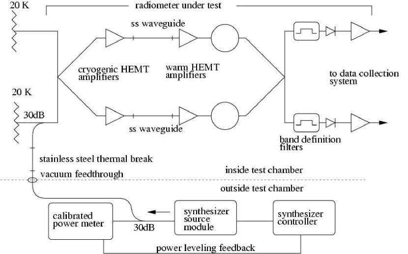
Figure 9: Test setup used to measure the radiometer’s bandpasses. The calibrated power meter and synthesizer are configured to provide a constant power at the output of the room temperature 30 dB coupler. The parameters of this coupler, and all the fixturing waveguide used to route the signal to the cold hybrid tee at the radiometer’s input were characterized with the VNA, and corresponding corrections applied to the measured bandpass data.

Measurements of the radiometers’ bandpasses are necessary for the analysis of in-flight data. Unlike the radiometric gains and offset, which are calibrated in flight, bandpass measurements must be made before launch. Measurements were made by injecting a small signal into the one port of the cold hybrid tee and recording the radiometric response. The level of the signal was set to yield a readily measurable radiometric response, but not so large as to cause non-linear effects. Figure 9 shows the test configuration used for these measurements. The VNA was used to make precise measurements of the frequency dependent transmission characteristics of all the components between the leveled source and radiometer’s input at the cold hybrid tee. The swept signal source was calibrated to produce a frequency independent power level at the output of the through port of the room temperature 30 dB coupler. The bandpass was measured by stepping the synthesized source through 201 frequencies, $\nu_{i}$, and recording the output of the radiometer at each frequency with the RF output of the synthesizer enabled and disabled. Differences between the data taken with the synthesizer on and off then yielded the radiometer’s response to the applied signal. Corrections were applied to these data to account for the frequency dependence of couplers and waveguide. Measurements were made at different power levels to ensure that non-linear effects arising from the large signal levels were not present.

The procedure resulted in a bandpass measurement relating the response from each detector to the input microwave power, referenced to the input port of the cold hybrid tee, so it does not include possible frequency dependences of the feed horn, OMT and waveguides connecting the OMT to the cold hybrid tees. The transmission coefficients of the OMT and waveguide sections were measured with the VNA and small ($<0.3$ dB) corrections applied to the measured responses, resulting in corrected responses, $r_{l}(\nu_{i})$ and $r_{r}(\nu_{i})$, for each detector.

Absolute calibration of the radiometers is performed in flight using observations of the CMB dipole. The demodulated digitized output of each detector, $y_{j}$, can be expressed as

$$y_{j}=y_{\mathrm{off},\,j}+y_{0,\,j}\sum_{i}r_{j}(\nu_{i})w_{A-B}(\nu_{i})$$ (36)

where $j=l,\,r$ designates the detector of the radiometer, $y_{\mathrm{off},\,j}$ is the radiometric offset, $y_{0,\,j}$, is the overall gain of the radiometer and data collection system, and $w_{A-B}(\nu_{i})$, is the power per unit bandwidth at frequency $\nu_{i}$ of the differential signal coupled to the radiometer’s input. Calibration is performed by comparing the change in each detector’s output signal, $\Delta y_{j}$, to the corresponding change in the input differential power signal arising from the CMB dipole :

$$\Delta y_{j} = y_{0,\,j}\left(\sum_{i}r_{j}(\nu_{i})w^{\prime}(\nu_{i})\right)\Delta(T_{A}-T_{B})$$ (37)

$$w(\nu) = \frac{h\nu}{e^{x}-1}$$ (38)

$$x = \frac{h\nu}{k_{B}T}$$ (39)

$$w^{\prime}(\nu) \equiv \left.\frac{1}{k_{B}}\frac{dw(\nu)}{dT}\right|_{T=T_{\mathrm{CMB}}}=\frac{x^{2}e^{x}}{(e^{x}-1)^{2}}.$$ (40)

Here $w(\nu)$ is the power per unit bandwidth delivered to a single mode by a blackbody at temperature $T_{CMB}=2.725$ K, $h$ is Planck’s constant, and $\Delta(T_{A}-T_{B})$ is the change in the differential thermodynamic temperature of the observed CMB dipole calculated from the orientation of the satellite. The calibration constants, $\widehat{r}_{j}$, are defined so that digitized data from each detector may be converted into measured thermodynamic temperature differences, $\Delta\widehat{T}_{\mathrm{\mathrm{th}},\,j}$, by

$$\Delta\widehat{T}_{\mathrm{\mathrm{th}},\,j}=\widehat{r}_{j}\Delta y_{j}.$$ (41)

The calibration constants are measured using the relation

$$\widehat{r_{j}}^{-1} = \left<\frac{\Delta y_{j}}{\Delta(T_{A}-T_{B})}\right>$$ (42)

$$= y_{0,\,j}\sum_{i}r_{l}(\nu_{i})k_{B}w^{\prime}(\nu_{i})$$ (43)

where the brackets indicate an average over many observations. The calibrated data of the two detectors are combined with a simple average to yield the calibrated radiometer output,

$$\Delta\widehat{T}_{\mathrm{th},\,\mathrm{avg}}=\frac{1}{2}(\widehat{r}_{l}\Delta y_{l}+\widehat{r}_{r}\Delta y_{r}).$$ (44)

The frequency response of this combined signal is an average of the two detector frequency responses

$$r_{\mathrm{avg}}(\nu_{i})=\frac{1}{2}\left(\frac{r_{l}(\nu_{i})}{\sum r_{l}(\nu_{i})w^{\prime}(\nu_{i})}+\frac{r_{r}(\nu_{i})}{\sum r_{r}(\nu_{i})w^{\prime}(\nu_{i})}\right).$$ (45)

Combined responses of representative radiometers in each of MAP’s frequency bands are presented in Figure 8.

Figure 8: Combined responses, $r_{\mathrm{avg}}(\nu)$, of representative radiometers in each of MAP’s five frequency bands. Note that the frequency ranges of the Ka and Q band radiometers overlap slightly.

The response of a radiometer to a signal with an arbitrary spectrum is obtained by integrating the product of $r_{\mathrm{avg}}(\nu)$ and the power spectrum over the passband of the radiometer. The factors used to convert thermodynamic temperature differences to Rayleigh-Jeans temperature differences for the calibrated radiometer output were calculated using the relation

$$\frac{d(\Delta\widehat{T}_{\mathrm{th},\,\mathrm{avg}})}{dT_{\mathrm{RJ}}}=\frac{\sum r_{\mathrm{avg}}(\nu_{i})}{\sum r_{\mathrm{avg}}(\nu_{i})w^{\prime}(\nu_{i})}$$ (46)

and are listed in Table 11. The numerator on the right hand side of equation 46 is uniformly weighted with frequency since the power per unit bandwidth in Rayleigh-Jeans units is independent of frequency. The thermal center frequency for each radiometer, $\nu_{\mathrm{th}}$, is the frequency at which the Rayleigh-Jeans to thermodynamic conversion equals that calculated for the radiometer,

$$\frac{d(\Delta\widehat{T}_{\mathrm{th},\,\mathrm{avg}})}{dT_{\mathrm{RJ}}}=\frac{1}{w^{\prime}(\nu_{\mathrm{th}})}$$ (47)

and are also given in Table 11. The factors need to convert an observed Rayleigh-Jeans temperature difference to a Rayleigh-Jeans temperature difference at another frequency, $\nu_{0}$, for objects with antenna temperature scaling as $T_{A}\propto\nu^{\beta}$ were calculated from the relation

$$\frac{dT_{\mathrm{RJ}}}{dT_{\mathrm{RJ}}(\nu_{0})}(\beta)=\frac{\sum r_{\mathrm{avg}}(\nu_{i})(\frac{\nu_{i}}{\nu_{0}})^{\beta}}{\sum r_{\mathrm{avg}}(\nu_{i})}.$$ (48)

In these units a source with a constant Rayleigh-Jeans temperature has $\beta=0.$ The resulting coefficients were fit to a function of the form

$$\frac{dT_{\mathrm{RJ}}}{dT_{\mathrm{RJ}}(\nu_{0})}(\beta)=\left(\frac{\nu_{\mathrm{avg}}}{\nu_{0}}\right)^{\beta}(1+c_{1}\beta+c_{2}\beta^{2})$$ (49)

for $-3<\beta<1$ and the resultant parameters, $\nu_{\mathrm{avg}}$, $c_{1}$ and $c_{2}$ are given in Table 11.

These quantities apply to diffuse sources that completely fill the beams of the instrument. For resolved sources additional terms resulting from the frequency dependent beam sizes must be included (Page, 2003). Tabulated bandpass measurements will be made available as part of the MAP data release.

Table 11: MAP Radiometer Bandpass Parameters

Radiometer	$\nu_{\mathrm{avg}}\ (\mbox{$\textrm{GHz}$})$	$c_{1}$	$c_{2}$	$\Delta\nu_{eff}\ (\mbox{$\textrm{GHz}$})$	$\nu_{\mathrm{th}}(\mbox{$\textrm{GHz}$})$	$dT_{\mathrm{th}}/dT_{\mathrm{RJ}}$
K11	22.29	-2.43E-03	2.78E-03	5.26	22.36	1.013
K12	23.12	-2.35E-03	2.83E-03	4.09	23.18	1.014
Ka11	32.78	-1.58E-03	1.75E-03	6.75	32.84	1.028
Ka12	33.12	-1.85E-03	2.06E-03	7.04	33.19	1.029
Q11	40.71	-1.85E-03	2.10E-03	8.62	40.79	1.044
Q12	40.81	-1.48E-03	1.70E-03	7.66	40.88	1.044
Q21	40.16	-1.58E-03	1.78E-03	7.55	40.23	1.043
Q22	40.92	-1.53E-03	1.78E-03	7.68	40.99	1.044
V11	59.20	-2.13E-03	2.20E-03	8.37	59.32	1.095
V12	61.10	-2.00E-03	2.23E-03	12.53	61.22	1.101
V21	61.61	-1.95E-03	2.22E-03	12.81	61.72	1.103
V22	60.63	-2.12E-03	2.35E-03	11.66	60.75	1.099
W11	93.60	-2.02E-03	2.20E-03	20.81	93.71	1.249
W12	93.18	-1.69E-03	1.82E-03	18.30	93.27	1.247
W21	93.49	-1.47E-03	1.57E-03	16.54	93.58	1.248
W22	94.27	-1.37E-03	1.48E-03	16.54	94.35	1.253
W31	92.36	-1.35E-03	1.44E-03	16.70	92.44	1.242
W32	93.32	-1.30E-03	1.37E-03	16.15	93.39	1.247
W41	94.24	-1.67E-03	1.83E-03	18.76	94.33	1.253
W42	93.09	-1.58E-03	1.68E-03	17.73	93.18	1.246

8 Summary

The design, assembly, and test procedures for the 20 differential microwave radiometers comprising MAP have been described. Through the use of rapid phase switching and instantaneous differencing radiometer instabilities arising from the HEMT amplifiers’ gain fluctuations have been dramatically reduced. Ground characterization tests indicate that the MAP radiometers and support electronics will meet MAP’s sensitivity and systematic error goals when operating in flight.

9 Acknowledgments

The MAP radiometers are the result of countless hours of work by many dedicated individuals. N. Bailey, T. Boyd, R. Harris, W. Lakatosh, D. Thacker, J.Webber , and B. Wireman at NRAO produced the remarkable HEMT amplifiers which are the heart of this project. The National Radio Astronomy Observatory is a facility of the National Science Foundation operated under cooperative agreement by Associated Universities, Inc. A. Hislop of Pacific Millimeter Projects and H. Arain of Microwave Resources Inc. worked closely with MAP to produce the phase switches and filters. D. Bergman, D. Brigham, J. Caldwell, and C. Kellenbenz of NASA/GSFC were responsible for the radiometer support electronics. M. Jones and M. Delmont of NASA/GSFC provided essential quality assurance oversight to Princeton, NRAO and numerous component vendors. C. Jackson was invaluable as instrument system engineer in coordinating the efforts of the different groups. At Princeton technical support was provided by R. Bitzer, W. Groom, R. Sorenson, and C. Sule. G. Atkinson, W. Dix, J. Mellodge and L. Varga in the Princeton machine shop worked on both the radiometer test facilities and the flight hardware. Administrative and purchasing services at Princeton were provided by S. Dawson, H. Murray, A. Qualls, and K. Warren. This research was supported by the MAP project under the NASA Office of Space Science and Princeton University.

Appendix A Detector Noise Covariance

Consider the situation where two uncorrelated voltage noise sources, $u_{1}$ and $u_{2}$, are connected to the inputs of a hybrid tee, and two square law detectors are connected to the output as shown in Figure 10. The voltage noise at the input to the two detectors becomes

$$\frac{u_{1}+u_{2}}{\sqrt{2}}\ \textrm{and}\ \frac{u_{1}-u_{2}}{\sqrt{2}}.$$ (A1)

The output voltages of the two square law detectors are proportional to the squares of these quantities, with proportionality constants $s_{l}$ and $s_{r}$ for the two detectors. The covariance between the two detector outputs is

$$\overline{(V_{l}-\overline{V_{l}})(V_{r}-\overline{V_{r}})} = \left(\overline{(V_{l}V_{r})}-\overline{V_{l}}\ \overline{V_{r}}\right)$$ (A2)

$$= \frac{s_{l}s_{r}}{4}\left(\overline{(u_{1}+u_{2})^{2}(u_{1}-u_{2})^{2}}-\overline{(u_{1}^{2}+u_{2}^{2})}^{2}\right)$$ (A3)

$$= \frac{s_{l}s_{r}}{4}\left((\overline{u_{1}^{4}}+\overline{u_{2}^{4}}-2\overline{u_{1}^{2}u_{2}^{2}}-(\overline{u_{1}^{2}}+\overline{u_{2}^{2}})^{2}\right).$$ (A4)

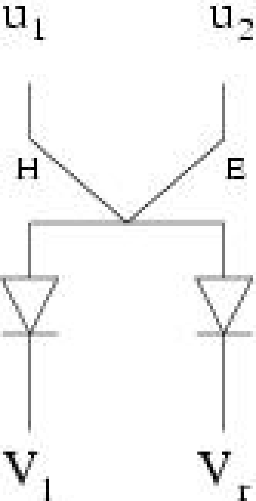
Figure 10: Noise sources and detectors attached to a hybrid tee. E and H are labels for the arms of the hybrid tee.

For a normally distributed variable, such as $u_{i}^{2}$, we have $\overline{u_{i}^{4}}=3\overline{u_{i}^{2}}^{2}$, so

$$.\overline{(V_{l}-\overline{V_{l}})(V_{r}-\overline{V_{r}})}=\frac{s_{l}s_{r}}{4}2(\overline{u_{1}^{2}}^{2}+\overline{u_{2}^{2}}^{2}-2\overline{u_{1}^{2}u_{2}^{2}})=\frac{s_{l}s_{r}}{2}\left(\overline{u_{1}^{2}}-\overline{u_{2}^{2}}\right)^{2}$$ (A5)

References

- Barnes (2002) Barnes et al. 2002, ApJS, 143, 567
- Bennett et al. (2003) Bennett et al. 2003, ApJ, 583, in press
- Dicke (1946) Dicke, R.H. 1946, Rev. Sci. Instrum., 17, 268
- Jarosik (1996) Jarosik, N.C., IEEE Transactions on Microwave Theory and Techniques 1996, 44, 193
- Kogut et al. (1996) Kogut et al. 1996, ApJ, 470, 653
- Kraus (1986) Kraus, J.D. 1986, Radio Astronomy 2nd Ed., Powell, Ohio, Cygnus-Quasar Books
- Page (2003) Page et al. 2003 ApJ, 585, in press
- Pospieszalski (2000) Pospieszalski, M. P., Wollack, E.J., Bailey, N., Thacker, D., Webber, J. 2000, IEEE MTT-S International Microwave Symposium Digest, Boston, MA, 1, 25
- Predmore (1985) Predmore, C.R. et al. 1985, IEEE Transactions on Microwave Theory and Techniques, 33, 356
- Wedge (1992) Wedge, S.W. & Rutledge, D.B. 1992, IEEE Transactions on Microwave Theory and Techniques, 40
- Wollack (1998) Wollack, E.W. & Pospieszalski, M.W., Proc. 1998 IEEE MTT-S Int. Microwave Symp. Digest, Baltimore, MD, p 669