Disk-Bulge-Halo Models for the Andromeda Galaxy

Abstract

We present a suite of semi-analytic disk-bulge-halo models for the Andromeda galaxy (M31) which satisfy three fundamental conditions: (1) internal self-consistency; (2) consistency with observational data; and (3) stability of the disk against the formation of a central bar. The models are chosen from a set first constructed by Kuijken and Dubinski. We develop an algorithm to search the parameter space for this set in order to best match observations of the M31 rotation curve, inner velocity dispersion profile, and surface brightness profile. Models are obtained for a large range of bulge and disk masses; we find that the disk mass must be $\lesssim 8\times 10^{10}\,M_{\odot}$ and that the preferred value for the bulge mass is $2.5\times 10^{10}\,M_{\odot}$. N-body simulations are carried out to test the stability of our models against the formation of a bar within the disk. We also calculate the baryon fraction and halo concentration parameter for a subset of our models and show that the results are consistent with the predictions from cosmological theories of structure formation. In addition, we describe how gravitational microlensing surveys and dynamical studies of globular clusters and satellites can further constrain the models.

1 Introduction

Owing to its size, proximity (distance $\sim 770$ kpc), and long history of observation, the Andromeda galaxy (M31) offers a unique opportunity to study in detail the components of a large spiral (Sb) galaxy. The aim of this paper is to present new disk-bulge-halo models for M31 that are (1) internally self-consistent; (2) consistent with published observations within $30\,{\rm kpc}$; and (3) stable against the rapid growth of bar-like modes in the disk. Our models are drawn from a general class of three-component models constructed by Kuijken & Dubinski (1995, hereafter KD), chosen to fit available observations of the M31 rotation curve, surface brightness, and bulge velocity profiles. The models span a parameter space defined by the disk and bulge masses, flattening parameter and tidal radius of the galactic halo.

One advantage of the KD models is that they provide the full phase-space distribution function (DF) for each of the components. The DFs are simple functions of three integrals of motion: the energy, the angular momentum, and an approximate integral which describes the vertical motions of particles in the disk. This feature insures that the models are (very nearly) in dynamical equilibrium. The KD models are each specified by 15 parameters. Of these, 10 have a direct effect on the rotation curve, velocity dispersion, and surface brightness profile of the model galaxy. A search of this parameter space yields a set of models that fit the observational data to within quoted uncertainties.

The data considered in this paper constrain the inner $\sim 30\,{\rm kpc}$ of M31 but say little about the mass distribution at larger radii. For this, one must turn to dynamical tracers such as dwarf satellites (Mateo, 1998; Evans et al., 2002) and globular clusters (Perrett et al., 2002). Recently Evans & Wilkinson (2000) derived an estimate for the total mass of M31 based on observations of satellites and outer halo globular clusters. Their analysis assumed simple analytic forms for the gravitational potential of M31 and the DFs of the tracer populations. The models and methods presented in this paper may provide the basis for future investigations along similar lines and, in particular, a unified and self-consistent treatment of the full data set associated with M31.

Two gravitational microlensing surveys toward M31 are currently underway (Crotts et al., 2001; Crotts & Tomaney, 1996; Kerins et al., 2001; Calchi Novati et al., 2002). Similar surveys toward the Magellanic Clouds have so far yielded inconclusive results. Roughly 20 microlensing events have been observed toward the LMC and SMC (Alcock et al., 2000; Lasserre et al., 2000), but one cannot say whether the lenses responsible for these events are indeed MACHOs or simply stars within the Magellanic Clouds or Milky Way disk. The M31 microlensing experiments should be able to resolve this question. M31 is highly inclined and therefore lines of sight toward the far side of its disk pass through more of its halo than do lines of sight toward the near side. If the halo of M31 is composed (at least in part) of MACHOs, there will be more microlensing events occurring toward the far side of the galaxy (Crotts, 1992). Previous efforts to compute theoretical optical depth and event rate maps for M31 assumed ad hoc models for the disk, bulge, and halo. Our models represent a significant improvement over these models since they are both internally self-consistent and are consistent with published data on M31. We will describe how one can compute optical depth and event rate maps for the models constructed in this study.

This paper takes the following form. In Section 2 we review published observations of the rotation curve, velocity dispersion profile, and surface brightness profile of M31. Section 3 provides a summary of the main features of the KD models. In Section 4, we describe a method to search parameter space for models which best fit the observations. The results of this search are presented in Section 5. Promising models are found which span a wide range in disk mass and in halo tidal radius and shape. We compute various properties of these models such as the disk and bulge mass-to-light ratios and the baryon mass fraction. For a subset of the models, we calculate the mass distribution and line-of-sight velocity dispersion profiles. We also fit the density profile to the NFW profile (Navarro, Frenk & White, 1996) and thus obtain an estimate for the halo concentration parameter. In Section 6, we describe a technique to construct theoretical event rate maps and present one example. Our conclusions and a discussion of possible extensions of this work are presented in Section 7.

2 Observations

Our analysis utilizes published measurements of the galaxy’s rotation curve, average surface brightness profile, and bulge velocity profiles. There is a considerable amount of M31 observational data of dissimilar quality available from the literature. In this section, we briefly describe the data selected for use in fitting the KD models.

2.1 Rotation Curve

Rotation curves for the M31 disk have been obtained from optical and radio observations spanning various ranges in galactocentric radius (e.g., Rubin & Ford, 1970, 1971; Gottesman & Davies, 1970; Deharveng & Pellet, 1975; Kent, 1989; Braun, 1991). An optimal combination of such data sets requires a good understanding of any associated calibration errors and uncertainties. In this study, the composite rotation curve for the galaxy was obtained by combining velocity data from the studies of Kent (1989) and Braun (1991). Kent (1989) obtained velocities with estimated statistical errors of $\sim 6\,{\rm km\,s^{-1}}$ for 30 HII emission regions along the major axis of the galaxy, with galactocentric radii in the range of 6 – 25 kpc. The Braun (1991) measurements of neutral hydrogen within the gaseous disk of M31 yielded velocity measurements out to a radius of $r\sim 30$ kpc. Braun’s data within 2 kpc of the M31 center were neglected here due to possible distortions arising from the presence of a bar-like triaxial ellipsoidal bulge. Beyond $r\sim 20$ kpc, measurements were obtained for spiral arm segments on only one side of the galaxy, hence data in this region were also not incorporated into our fitting. Details of the rotation curve interpolation can be found in (Braun, 1991).

Both sets of rotation velocity measurements and their respective errorbars are shown in the upper panel of Figure 1. Kernel smoothing was used to form the composite disk rotation curve, which is shown with its RMS uncertainties in the lower panel of Figure 1.

In determining the rotation curve of the galaxy, Braun assumes circular gas motions within the disk. It should be noted that the presence of certain dynamical anomalies may lead to systematic errors in the rotation curve determination. Such anomalies will be discussed at the end of Section 3.

2.2 Surface Brightness Profile

Although there have been many optical photometric studies of M31 (see, for example, Table 4.1 of Walterbos & Kennicutt, 1987), the task of combining such data sets is not straightforward. Differences in filter bandpasses and resolution between the various studies yield systematic errors which are generally difficult to characterize. Discrepancies in the adopted galaxy inclination and isophote orientation also contribute to differences in the light profiles obtained by different authors. For these reasons, we opted to avoid combining different data sets and instead adopted the surface brightness profile from Walterbos & Kennicutt (1987). These authors produced a global light profile for M31 out to $r\sim 28$ kpc by averaging the distribution of galaxy light over elliptical rings, assuming an inclination of $77^{\circ}$. The inner parts of the galaxy are dominated by light from the bulge component, which itself has a significantly higher position angle (PA) than that of the disk: ${\rm PA}\sim 50^{\circ}$ versus $38^{\circ}$ (Hodge & Kennicutt, 1982).

There is a distinct variation in the position angle of elliptical isophotes fitted to the surface brightness of M31 as one looks out in galactocentric radius (Hodge & Kennicutt, 1982). Furthermore, there is a significant warp in the disk beyond $r\sim 22\,{\rm kpc}$ (Walterbos & Kennicutt, 1987). These structural features cannot be reproduced in the KD models and will thus contribute to fitting errors calculated for the surface brightness profiles.

2.3 Bulge Velocity Profiles

The dynamics of the bulge can be used to deduce the mass distribution in that component of the galaxy. We utilize the stellar rotation and velocity dispersion results of McElroy (1983) along the bulge major axis (${\rm PA}=45^{\circ}$) and minor axis (${\rm PA}=135^{\circ}$) in the fits to the KD models described later in Section 3. The bulge data were smoothed using the same kernel averaging technique mentioned above; the rotation and dispersion results are shown in Figures 2 and 3, respectively.

McElroy (1983) noted several asymmetries in the rotation curves along various position angles of the bulge for $|R|<10^{\prime}$, although the cause of these asymmetries was unclear. The KD models are unable to reproduce such asymmetries within the bulge; we will return to this point later in the next section.

3 Self-Consistent Disk-Bulge-Halo Models

Kuijken & Dubinski (1995) constructed a set of semi-analytic models for the phase-space DFs of disk galaxies. Their models have three components: a thin disk, a centrally concentrated bulge, and an extended halo. In this section we summarize the essential features of these models.

The halo DF is taken to be a lowered Evans model (Kuijken & Dubinski, 1994). Evans models (Evans, 1993) are exact, two-integral distribution functions for the flattened logarithmic potential, $\Psi\propto\log{\left(x^{2}+y^{2}+z^{2}/q^{2}\right)}$ where $q$ is the flattening parameter. As with the isothermal sphere, Evans models are infinite in extent. In analogy with the lowered isothermal sphere or King model (King, 1966), lowered Evans models introduce a truncation in energy such that the system that results has finite mass. The halo DF

$$f_{\rm halo}\left(E,\,L_{z}\right)=\left\{\begin{array}[]{ll}\left[\left(AL_{z}^{2}+B\right)\exp{\left(-E/\sigma_{0}^{2}\right)}+C\right]\left(\exp\left(-E/\sigma_{0}^{2}\right)-1\right)&\mbox{if $E<0$}\\ 0&\mbox{otherwise}\end{array}\right.$$ (1)

has five free parameters: $A,\,B,\,C,\,\sigma_{0},\,$ and $\Psi_{0}$, the central potential for the system. Following KD, the first three parameters are replaced by $q$, a characteristic halo radius $R_{a}$, and a core radius $R_{c}$. In practice, the latter is described in terms of a core smoothing parameter $\left(R_{c}/R_{K}\right)^{2}$, which specifies the ratio of the core radius to the derived King radius for the halo. The DF is independent of the sign of $L_{z}$ and may therefore be written as the sum of two components, one with positive $L_{z}$ and the other with negative $L_{z}$. Rotation can be incorporated into the model by varying the relative “weight” of these two parts as specified through the streaming fraction $S_{h}~{}(=1/2~{}{\rm for~{}no~{}rotation})$.

The bulge DF is given by the lowered isothermal sphere or King model (King, 1966; Binney & Tremaine, 1987), and takes the form

$$f_{\rm bulge}\left(E\right)=\left\{\begin{array}[]{ll}\rho_{b}\left(2\pi\sigma_{b}^{2}\right)^{-3/2}\exp{\left[\left(\Psi_{0}-\Psi_{c}\right)/\sigma_{b}^{2}\right]}\left(-\exp{\left[\left(E-\Psi_{c}\right)/\sigma_{b}^{2}\right]}-1\right)&\mbox{if $E<\Psi_{c}$}\\ 0&\mbox{otherwise}\end{array}\right.$$ (2)

where $\rho_{b}$ and $\sigma_{b}$ govern the central density and velocity dispersion of the bulge. The cut-off potential, $\Psi_{c}$, controls the extent of the bulge. As with the halo, there is an additional parameter, the bulge streaming fraction $S_{b}$, which controls the rotation of the bulge.

The disk DF depends on three integrals of motion: $E$, $L_{z}$, and an approximate third integral corresponding to the energy associated with vertical oscillations of stars in the disk. The disk DF can be chosen to yield a density field with the desired characteristics. In the KD models, the density falls off approximately as an exponential in the radial direction and as ${\rm sech}^{2}$ in the vertical direction. Five parameters are used to characterize the disk: its mass $M_{d}$, the radial scale length $R_{d}$, the scale height $h_{d}$, the disk truncation radius $R_{o}$, and the parameter $\delta R_{o}$ which governs the sharpness of the truncation.

In a given potential, the DF for each component implies a unique density field. For self-consistency, the density-potential pair must satisfy the Poisson equation. This is accomplished by an iterative scheme as described by Kuijken & Dubinski (1995). The essential point is that the properties of the density fields of the bulge and halo are implicit rather than explicit functions of the input parameters. In particular, the masses of the bulge and halo ($M_{b}$ and $M_{h}$, respectively) and the halo tidal radius ($R_{t}$) are determined a posteriori. Likewise, the shapes of the bulge and halo are determined via the Poisson-solving algorithm. In particular, the bulge is flattened due to the contribution to the potential from the disk.

By design, the KD models are axisymmetric and therein lies the main limitation to the development of a truly realistic model for M31. Observational studies indicate that M31 cannot be described adequately by an axisymmetric model. Dynamical anomalies for M31 include factors such as the presence of a triaxial bulge (Stark, 1977; Gerhard, 1986), perturbations caused by its companions M32 and NGC 205 (Byrd, 1978; Sato & Sawa, 1986), the effects of significant variations in the inclination of the galactic plane as a function of radius (Hodge & Kennicutt, 1982), areas of infall motion towards the galaxy center (Cram, Roberts & Whitehurst, 1980), and local anomalies attributable to fine structure and shocks within the spiral arms of the galaxy (Braun, 1991). Small local perturbations in spectra obtained through dust lanes in the central regions of the galaxy may also be a factor. These dust patches would have the effect of slightly increasing the local radial velocity measurements, thereby inducing local errors in the rotation curve of the bulge (McElroy, 1983). Furthermore, the bulge dispersion may be affected by residual rotation caused by disk contamination along its minor axis.

4 Fitting KD Models to the Observations

The KD models are specified by 15 parameters: four for the bulge, five for the disk and six for the halo. Our goal is to determine the parameter set that yields a model which best fits the observations. This is accomplished by minimizing the composite $\chi^{2}$ statistic that is calculated by comparing the model rotation curve, surface brightness profile, and bulge velocity profiles with the data sets as described in Section 2.

4.1 Minimization Strategy

Unfortunately, the data considered in this paper are not sufficient to determine a global minimum in the full 15-dimensional parameter space. We therefore adopt a strategy in which a best-fit model is found for targeted values of the disk and bulge masses, flattening parameter, and in some cases, tidal radius. In addition, we do not attempt to minimize over the disk thickness, disk truncation radius, or halo streaming fraction (i.e., the parameters $R_{o}$, $\delta R_{o}$, $h_{d}$, or $S_{h}$). Our analysis proceeds as follows:

1. The surface brightness profile at radii where the disk dominates is very nearly exponential. In the R-band, the scale radius of the disk is $5.4\,{\rm kpc}$. We therefore fix $R_{d}$ to this value at the outset.

2. Since the data used in our analysis have little to say about the parameters $R_{o}$, $\delta R_{o}$ and $h_{d}$, we set them to be typical values for M31 of $40\,{\rm kpc}$, $1\,{\rm kpc}$, and $300\,{\rm pc}$, respectively. In addition, we assume that the halo does not rotate, i.e., $S_{h}=0.5$.

3. We consider models with disk and bulge masses in the following ranges:

   $$3\times 10^{10}\,M_{\odot}\leq M_{d}\leq 16\times 10^{10}\,M_{\odot}$$

   $$1\times 10^{10}\,M_{\odot}\leq M_{b}\leq 4\times 10^{10}\,M_{\odot}~{}.$$

   $M_{d}$ is an input parameter but $M_{b}$ is a complicated function of $\rho_{b}$, $\sigma_{b}$, $\Psi_{c}$ and, to a lesser extent, the other parameters. Therefore, to force the minimization routine to select a model with the desired $M_{b}$, we minimize a “pseudo-$\chi^{2}$ statistic” that includes the term $\left(M_{b}\left({\rm desired}\right)-M_{b}\left({\rm model}\right)\right)^{2}/\sigma_{M_{b}}^{2}$. The user-specified parameter $\sigma_{M_{b}}$ controls the accuracy with which $M_{b}$ is fit to the desired value. Of course, the physically relevant quantity is the $\chi^{2}$ statistic associated with the fits to the observational data, and this is the one quoted herein.

4. As with $M_{b}$, the tidal radius of the halo is an implicit function of the other input parameters. Therefore, for those cases where we wish to specify the tidal radius, an additional term $\left(R_{t}\left({\rm desired}\right)-R_{t}\left({\rm model}\right)\right)^{2}/\sigma_{R_{t}}^{2}$ is included as part of the pseudo-$\chi^{2}$ statistic in order to drive $R_{t}$ to the desired value. Again, the user specifies the value of $\sigma_{R_{t}}^{2}$.

5. The flattening parameter $q$ governs the shape of the halo potential and is specified explicitly. The shape of the mass distribution of the halo is determined implicitly through the Poisson-solving algorithm.

A given model is constructed by minimizing the pseudo-$\chi^{2}$ statistic for the fit. This minimization procedure is described in the next section.

4.2 Multidimensional Minimization Technique

Minimization of the pseudo-$\chi^{2}$ statistic over the multidimensional KD parameter space is performed by employing the downhill simplex algorithm (see, for example, Press et al., 1986). An N-dimensional simplex is a geometrical object consisting of $N+1$ points or vertices and all of the line segments that connect them. Thus, a simplex encloses a finite volume in an N-dimensional space. For the case at hand, the space is defined by the 10 free parameters as described above. An initial guess at the values of these parameters fixes one vertex of the initial simplex. The remaining vertices of the initial simplex are constructed by stepping in each direction of parameter space by some appropriate distance, which is typically set to 10% of the parameter value.

The downhill simplex algorithm proceeds through a series of iterations as follows. The pseudo-$\chi^{2}$ statistic is calculated at each vertex of the simplex. The algorithm then reflects the vertex with the highest value of pseudo-$\chi^{2}$ through the opposite face of the simplex to search for a lower function value. If a lower value is found at this new location, the algorithm proceeds by testing the point twice as far along this line. The vertex in the original simplex with the highest pseudo-$\chi^{2}$ is then replaced by the reflected position with the lower function value. If a lower value is not found at the reflected position, the simplex is contracted about its vertex with the lowest function value. In this manner, the simplex steps through parameter space and gradually contracts around the point with the minimum pseudo-$\chi^{2}$, thereby honing in on the best fit to the observed data and the targeted values for the component masses and/or tidal radius.

The downhill simplex method has a number of advantages over minimization procedures that are based on gradients of the function (e.g., the method of steepest descent; see Press et al. (1986) and references therein). Gradient methods appear to be more susceptible to the presence of local minima in the complicated $\chi^{2}$ surface. In addition, the simplex method is computationally efficient, requiring relatively few function evaluations. Between 10 and 100 iterations are needed in order to locate a position in parameter space with the minimum value of pseudo-$\chi^{2}$. An iteration requires between 1 and 10 function evaluations, each of which takes a minute or so of CPU time. Therefore, a model can typically be generated within $1-2$ CPU-hours using a standard 1 GHz desktop computer.

5 The Models

We begin with a survey of models in the $M_{d}-M_{b}$ plane focusing on the quality of the fits to the observational data, the stability of the disk, and the mass-to-light ratios of the disk and bulge components. We next consider constraints on the mass distribution beyond $30\,{\rm kpc}$ from dynamical studies of satellite galaxies, globular clusters, and planetary nebulae. We also check whether our preferred models are consistent with predictions from the baryonic Tully-Fisher relation and cosmological constraints such as the baryon fraction. Toward this end we construct a series of models with tidal radii between $80\,{\rm kpc}$ and $160\,{\rm kpc}$ and also explore the implications of replacing the lowered Evans halo of a KD galaxy, which has a sharp cut-off in density at the tidal radius, with an NFW halo. Finally, we investigate models with flattened halos, such that $q<1$.

5.1 The Disk and Bulge Mass Models

We have constructed and analysed over twenty M31 models in the $M_{b}-M_{d}$ plane with $q=1$ and $R_{t}$ unconstrained. Table 1 summarizes the results for a select subset of these models. In addition to the disk and bulge masses, Table 1 provides the composite $\chi^{2}$ statistic for the fits to the observational data (column 4), the R-band mass-to-light ratios for the disk and bulge (columns 5 and 6), the mass interior to a sphere 30 kpc in radius (column 7), the mass of the halo (column 8) and the tidal radius (column 9).

Our analysis indicates that there is a trough in $\chi^{2}$ running roughly parallel to the $M_{d}$-axis and centered on $M_{b}\simeq 2.5\times 10^{10}\,M_{\odot}$. Both Models A and D lie near the minimum of this trough while Models A, B, and C trace out the cross section of the trough at $M_{d}=7\times 10^{10}\,M_{\odot}$. Models along the minimum of the trough have low values of $\chi^{2}$ (typically $\chi^{2}\simeq 0.6-1$) indicating an excellent overall fit to the observations. This point is illustrated in Figures 4 and 5 where we compare the theoretical predictions for Models A and D with the observational data. The agreement is particularly good for the gas rotation curve and inner velocity dispersion profiles along the galaxy’s major and minor axes. Furthermore, the exponential disk does an excellent job of fitting the surface brightness profile beyond $5\,{\rm kpc}$ though the fit is not as good in the transition zone between bulge and disk dominated regions of the galaxy ($2\,{\rm kpc}\lesssim r\lesssim 4\,{\rm kpc}$). Moreover, the inner rotation curve for the model appears to have the wrong shape: the model curves are relatively flat while the data suggest a rotation curve that is rising slowly. These two discrepancies may, in part, reflect the fact that our models assume an axisymmetric bulge whereas the actual bulge of M31 is triaxial. We note that the mass distribution in the bulge component of the model is flattened — but still axisymmetric — due to its interaction with the gravitational potential of the disk. The major-to-minor axis ratio is found to be $\sim 0.8$, in good agreement with the value found by Kent (1989).

Figures 4 and 5 help to explain the existence of the trough in $\chi^{2}$. The contributions to the outer rotation curve ($r\gtrsim 5\,{\rm kpc}$) from the halo and disk are both rather broad in radius and therefore one can be played off the other.

Figure 5 shows that the disk dominates the rotation curve of Model D for $4\,{\rm kpc}\lesssim r\lesssim 30\,{\rm kpc}$. This feature, common to all high-$M_{d}$ models reveals a fundamental problem with these models, namely a susceptibility to the bar instability. A dynamically cold, self-gravitating disk is unstable to bar formation (Hohl, 1971) and since a strong bar instability completely disrupts the disk, any model in which one is present is unacceptable.

In general, bar instabilities can be suppressed by an extended halo, a bulge that dominates the dynamics of the inner part of the galaxy, significant vertical velocities among the disk stars, or a combination thereof (Ostriker & Peebles, 1973; Sellwood, 1985). We have performed a series of N-body experiments to test the stability of our models. We use the algorithm of Dehnen (2002), which has the advantage over tree and mesh codes in that the computation time scales as the number of simulation particles, $N$, rather than $N\ln{(N)}$. The simulations were performed with $2\times 10^{5}$ particles for each of the three components of the model and were run for 8 dynamical times as measured at one scale radius. Model D develops a bar within a few dynamical times as expected given that the disk dominates the gravitational potential within a radius of $r\sim 30\,{\rm kpc}$ (see Figure 5). Model A, in which the inner rotation curve is dominated by the bulge and the outer rotation curve is dominated by the halo (Figure 4), appears to be stable. These results are illustrated in Figure 6 where we show face-on and Milky-Way observer views of the evolved disk-particle distribution for Models A and D. Further simulations suggest that the demarcation between stable and unstable models occurs in the neighborhood of $M_{d}\simeq 8\times 10^{10}\,{\rm M}_{\odot}$. Models with a disk in this mass range show signs of weak spiral and bar-like structures (Stark, 1977). The presence of spiral structure in the disk of M31 as well as a triaxial bar-like bulge suggests that weak instabilities operate in this galaxy. Thus, $M_{d}=8\times 10^{10}\,{\rm M}_{\odot}$ should not be interpreted as a strict upper bound on the disk mass of M31 but rather as an interesting region of parameter space in which dynamical evolution may give rise to non-axisymmetric structures similar to what is observed in M31. What we can say for sure is that models like D and K1 are violently unstable and therefore ruled out. Conversely, Model K2 may be so stable that the mechanisms which drive spiral structure are suppressed (Sellwood, 1985).

Model K1 assumes values for $M_{d}$ and $M_{b}$ from the popular small-bulge model of Kent (1989). This model does a reasonable job of fitting the surface brightness profile as well as the rotation curve beyond $6\,{\rm kpc}$ (Figure 7). However, Model K1 predicts a velocity dispersion in the bulge region that is too large. This discrepancy is common among all models with $M_{b}\simeq 4\times 10^{10}\,M_{\odot}$ (e.g., Models C and K2). It is already evident in Figure 3 of Kent (1989) if one focuses on the McElroy (1983) data at $1-2\,{\rm kpc}$. The discrepancy is worse for the self-consistent models considered here. Kent assumed a constant density halo: when compared with a realistic model halo (i.e., one in which the density is monotonically falling with radius) the contribution to the rotation curve from a constant density halo is relatively low at small radii. For a fixed halo contribution to $v_{\rm circ}^{2}$ at $30\,{\rm kpc}$, Kent’s model underestimates the halo contribution in the region of the bulge as compared with more realistic models.

Model K2 assumes values for $M_{d}$ and $M_{b}$ used in the pixel-lensing study from Kerins et al. (2001). This model provides an excellent fit to the surface brightness profile, matching almost perfectly the data through the transition zone between bulge and disk dominated regions of the galaxy (Figure 8). However the model rotation curve appears to have the wrong shape between $7$ and $12\,{\rm kpc}$ and perhaps also beyond $20\,{\rm kpc}$. In addition, the model velocity dispersion profile is systematically high, as discussed above. (Note that in Kerins et al. (2001), where the density profile of the halo is taken to be that of a cored isothermal sphere, the model rotation curve provides a good fit to the data.)

5.2 Mass-to-Light Ratios

We now consider the disk and bulge mass-to-light ratio for the models in Table 1 (see columns 5 and 6). The $(M/L_{R})$ values for Model K1 are in excellent agreement with the results obtained by Kent (1989), who found $\left(M/L_{r}\right)_{d}=10$ and $\left(M/L_{r}\right)_{b}=5$. This agreement serves as a consistency check of our method though it is worth noting that Kent uses the r-band filter of the Thuan & Gunn system which differs slightly from the R-band filter of the standard UBVRI system used by Walterbos & Kennicutt (1987) (see Table 2.1 of Binney & Merrifield (1998) for a comparison of the different filter characteristics).

As expected, the disk and bulge $M/L$ values for the other models in Table 1 scale roughly with the mass of the corresponding component. In particular, the $M/L$ values for Model A are approximately a factor of two smaller than those for Model K1. The values for Model A compare well with the predictions from stellar synthesis studies. Bell & de Jong (2001) presented a correlation between the stellar mass-to-light ratios and the optical colors of integrated stellar populations for spiral galaxies. Based on the relationships they obtained under different assumptions of initial mass function combined with typical M31 disk and bulge colors from Table 1 of Walterbos & Kennicutt (1988), one expects $M/L_{R}\sim 2-5$ within the different regions of M31.

Despite this general agreement between the model mass-to-light ratios and the predictions from stellar population studies, the question arises as to why, for all of the models of Table 1 except K2, $\left(M/L_{R}\right)_{d}$ is significantly greater than $\left(M/L_{R}\right)_{b}$. In general, one expects the mass-to-light ratio of the bulge to be comparable to, if not greater than, that of the disk (although see Héraudeau & Simien, 1997). We propose two explanations for this apparent difficulty. First, the quoted $M/L_{R}$ values presented in this paper do not incorporate corrections for foreground extinction. Since the effects of obscuration by dust are likely to be more severe in M31’s disk than in its bulge (Walterbos & Kennicutt, 1988), this correction would drive down the $M/L$ of the disk relative to that of the bulge and bring the two values more into line (Kent, 1989). Moreover, for typical Sb spirals like M31, gas contributes between 2 and 20% of the mass of the disk (see Figure 8.20 of Binney & Merrifield, 1998) and therefore boosts, by the same fraction, the $M/L$ value relative to the value for the stellar population. We therefore conclude that the values for $\left(M/L\right)_{d}$ and $\left(M/L\right)_{b}$ are quite reasonable.

It is nevertheless instructive to consider a second possibility, namely that the $M/L$ values obtained for Model A reflect a genuine problem that is perhaps be connected with the poor fit to the surface brightness profile in the disk-bulge transition region (Figure 4). Deviations of the structure of M31’s bulge from a simple oblate spheroid may also have resulted in an underestimate of its effective radius in the fitting procedure, causing the bulge to get somewhat short-changed in mass. One might then argue that Model K2 provides a superior fit to M31. However, the gains in the surface brightness profile and the in mass-to-light ratios made by employing Model K2 come at the cost of the quality of the rotation curve fit. Model K2 also has the unusual feature that the bulge mass is greater than the disk mass, contrary to what is commonly found for bright Sb galaxies.

5.3 Mass Distribution

The total mass interior to a sphere $30\,{\rm kpc}$ in radius, $M_{30}$, is provided in column 7 of Table 1. These values were obtained by generating an N-body realization of each model and tabulating the mass interior to the prescribed sphere. $M_{30}$ is constrained almost entirely by the outer rotation curve: a circular rotation speed at $30\,{\rm kpc}$ of $v_{r}\simeq 215\,{\rm km\,s^{-1}}$ (an average of the outer 4 points in Figure 1) corresponds to a mass estimate $v_{r}^{2}r/G=32\times 10^{10}\,M_{\odot}$. This is in good agreement with the values obtained for most of our models. The most prominent outlier is Model K2, where the model rotation curve rises to $v_{r}\simeq 265\,{\rm km\,s^{-1}}$ ($v_{r}^{2}r/G\simeq 50\times 10^{10}\,M_{\odot}$), in conflict with the observations.

Columns 8 and 9 of Table 1 provide the halo mass and tidal radius, respectively. Since the data considered in this paper probe only the inner $30\,{\rm kpc}$ of M31, it is not surprising that $M_{h}$ and $R_{t}$ vary considerably. Dynamical tracers such as globular clusters and dwarf galaxy satellites have been used to constrain the mass distribution of M31 beyond $r=30\,{\rm kpc}$. To better understand how this type of data might help constrain the models, we construct a sequence of models with $80\,{\rm kpc}\lesssim R_{t}\lesssim 160\,{\rm kpc}$, $q=1$, and $M_{d}$ and $M_{b}$ fixed to the values from Model A. The results for Model A ($R_{t}\simeq 80\,{\rm kpc}$) and Model E ($R_{t}\simeq 160\,{\rm kpc}$) are given in Table 2 for comparison. In addition to $\chi^{2}$, $R_{t}$, and $M_{h}$, we record the baryon fraction, $f_{B}$ (column 5). We also provide four quantities derived by substituting an NFW halo for the lowered Evans model. These quantities, to be discussed in Section 5.4, are the halo concentration parameter $c$ (column 6), the virial radius $R_{200}$ and mass $M_{200}$ (columns 7 and 8), and an alternate estimate for the baryon fraction based on the NFW halo, $f_{B,NFW}$ (column 9).

The value of $\chi^{2}$ is found to rise rapidly with increasing $R_{t}$. The main source of the discrepancy is with the rotation curve fits, as illustrated in Figure 9. Models with $R_{t}>160\,{\rm kpc}$ lead to even larger discrepancies between the predicted and observed rotation curves and thus provide completely unacceptable fits to the data.

Dynamical studies of globular clusters as well as planetary nebulae are especially useful for obtaining mass estimates at intermediate radii. Federici et al. (1993) analyzed spectroscopic observations for several dozen globular clusters in M31 between $10-30\,{\rm kpc}$, and derived a range for $M_{30}$ of $(50-80)\times 10^{10}\,M_{\odot}$. Using the projected mass estimator of Bahcall & Tremaine (1981) and Heisler, Tremaine & Bahcall (1985), Perrett et al. (2002) obtained a mass estimate of $\sim 40\times 10^{10}\,M_{\odot}$ based on data from 319 globular clusters out to $r\simeq 27\,{\rm kpc}$ and under the assumption of isotropic orbits. As with most mass estimates that are based on dynamical tracers, the uncertainty is due largely to our ignorance of the true orbit distribution for the globular cluster system.

Evans & Wilkinson (2000) considered a sample of M31 globular cluster candidates and planetary nebulae at large galactocentric radii and employed a more sophisticated method for estimating the mass of the galaxy. They assumed simple analytic forms for the globular cluster DF and for the halo-density-profile/gravitational-potential pair. Two parameters characterize their model potential and these were determined by performing a maximum likelihood analysis over the data. Evans & Wilkinson (2000) obtained a mass estimate at $r=40\,{\rm kpc}$ of $47\times 10^{10}\,M_{\odot}$ for the globular cluster data, while for the planetary nebulae data they found $M_{30}\simeq 28\times 10^{10}\,M_{\odot}$.

At present, virtually all of the information available for the outer halo of M31 comes from dynamical studies of its satellite galaxies. Courteau & van den Bergh (1999) used radial velocity data for Local Group members to calculate a dynamical mass of the Andromeda subgroup of $(133\pm 18)\times 10^{10}\,M_{\odot}$. Using data from high-resolution échelle spectroscopy from the Keck Telescope, Côté et al. (2000) applied the projected mass estimator to derive an M31 mass of $\sim 79\times 10^{10}\,M_{\odot}$ under the assumption of isotropic satellite orbits. In the cases of circular and radial orbits, the estimated enclosed masses change to $\sim 37\times 10^{10}\,M_{\odot}$ and $\sim 215\times 10^{10}\,M_{\odot}$, respectively. Based on the dynamical modelling of a similar set of data, Evans et al. (2000) obtained an M31 mass in the range of $(70-100)\times 10^{10}\,M_{\odot}$. For comparison, Evans & Wilkinson (2000) derived an estimate for the total mass of M31 within $\sim 550\,{\rm kpc}$ of $123^{+180}_{-60}\times 10^{10}\,M_{\odot}$. This result was obtained by applying the maximum likelihood DF method described above to the combined globular cluster, planetary nebula, and satellite data set.

In Figure 10 we plot the total mass distribution as a function of radius for the models listed in Table 2. The dynamical mass estimates described above are included for comparison. Based on these results, it would appear that both Models A and E provide adequate descriptions of the outer halo, with Model E coming closest to the estimates.

In a forthcoming publication, we will study in detail the constraints on our models from observations of dynamical tracers. Typically, for each member of the tracer population, one knows its angular position and line-of-sight velocity. As an illustration of how one might use such data, we show, in Figure 11, the line-of-sight velocity dispersion as a function of projected radius for Models A and E. The velocity dispersion along a particular line of sight as a function of the projected position vector ${\bf s}$, is given by

$$\sigma_{\rm LOS}^{2}\left({\bf s}\right)=\frac{1}{\Sigma\left({\bf s}\right)}\int_{l_{0}}^{\infty}dl\,\rho\left(l,{\bf s}\right)\langle v_{l}^{2}\left(l,{\bf s}\right)\rangle$$ (3)

where $l_{0}$ corresponds to the position of the observer and $\Sigma\left({\bf s}\right)=\int_{l_{0}}^{\infty}dl\rho\left(l,{\bf s}\right)$ is the surface density along the line of sight. The density $\rho\left(l,{\bf s}\right)$ and velocity dispersion $\langle v_{l}^{2}\left(l,{\bf s}\right)\rangle$ are calculated from the DF in the usual way:

$$\rho\left(l,{\bf s}\right)=\int d^{3}v\,f\left(l,{\bf s}\right)$$ (4)

and

$$\rho\left(l,{\bf s}\right)\langle v_{l}^{2}\left(l,{\bf s}\right)\rangle=\int d^{3}v\,v_{l}^{2}\,f\left(l,{\bf s}\right).$$ (5)

Here $v_{l}$ is the component of the velocity along the line of sight.

KD provide a simple algorithm that allows one to generate an N-body representation for any of their models. An N-body representation can be used to perform a Monte Carlo evaluation of the integrals in Eqs. 3, 4, and 5. The DF is written as a sum over the particles:

$$f\left({\bf x},\,{\bf v}\right)=m_{i}\sum_{i}\delta^{3}\left({\bf x}-{\bf x}_{i}\right)\delta^{3}\left({\bf v}-{\bf v}_{i}\right)$$ (6)

where $m_{i}$, ${\bf x}_{i}$, and ${\bf v}_{i}$ are the mass, position, and velocity of the $i^{\rm th}$ particle. The surface density is given by

$$\Sigma\left({\bf s}\right)=\sum_{i\in{\cal V}}m_{i}$$ (7)

where ${\cal V}$ is a volume corresponding to a thin tube centered on the line of sight. Likewise,

$$\sigma_{\rm LOS}^{2}\left({\bf s}\right)=\frac{1}{\Sigma\left({\bf s}\right)}\sum_{i\in{\cal V}}m_{i}v_{s,i}^{2}~{}.$$ (8)

The curves in 11 represent an average over position angle: differences between the line-of-sight dispersion profiles along the major and minor axes were found to be insignificant. Our results may be compared with those from the analytic halo-only model of Evans et al. (2000, see their Figure 3). More to the point, the model prediction for the line-of-sight velocity dispersion profile together with data for dynamical tracers can be incorporated into an improved version of our model-finding algorithm.

As a final consistency check, we turn to the Tully-Fisher relation (Tully & Fisher, 1977) which, in its original form, describes a tight correlation between the total luminosity of a spiral galaxy and $v_{\rm flat}$, the circular rotation speed in the flat part of the rotation curve. For our purposes, a variant known as the baryonic Tully Fisher relation (see McGaugh et al., 2000), which described a correlation between $v_{\rm flat}$ and the total baryonic mass in gas and stars, $M_{\rm baryons}$ is more useful. The baryonic Tully-Fisher relation takes the form

$$M_{\rm baryons}=A\,v_{\rm flat}^{b}$$ (9)

where $A$ and $b$ are constants. McGaugh et al. (2000) find that $b$ is statistically indistinguishable from $4$ (however, see (Bell & de Jong, 2001)) and that if it is fixed to this value, the normalization is $A\simeq 35\,h_{75}^{-2}M_{\odot}{\rm km^{-4}s^{4}}$ with large uncertianties (see for example, McGaugh (2001) where the acceptable range for $A$ is given as $34-85$ in units of $M_{\odot}{\rm km^{-4}s^{4}}$). For M31, $v_{\rm(30\,kpc)}\approx 230$ km s^-1 which implies, for a $A\simeq 35\,M_{\odot}{\rm km^{-4}s^{4}}$ baryonic mass of $9.8\times 10^{10}M_{\odot}$ in good agreement with the total baryon mass (taken to be $M_{d}+M_{b}$) in Model A. Note that somewhat higher values of $M_{d}$ can be tolerated without introducing too strong a bar instability. Thus, one would be able to find a consistent model even if a higher value of $A$ is assumed.

5.4 Connection with Cosmology

The baryon fraction can be used to constrain models of M31. In general, we expect the baryon fraction of a spiral galaxy such as M31 to be comparable to the baryon fraction of the Universe. Under the assumption that dark matter makes a negligible contribution to the mass of the disk and bulge, we have $f_{B}\leq\left(M_{d}+M_{b}\right)/\left(M_{d}+M_{b}+M_{h}\right)$ where $f_{B}$ is the baryon fraction of the galaxy as a whole. The inequality incorporates the possibility that some baryons may reside in the halo. Values for $f_{B}$ are given in column 8 of Table 2 and can be compared with estimates from cosmology and astrophysics. Based on Big Bang nucleosynthesis constraints, Burles, Nollett, & Turner (2001) derived an estimate of $\Omega_{B}h^{2}=0.020\pm 0.002$ where $\Omega_{B}$ is the density of baryons in units of the critical density and $h$ is the Hubble constant in units of $100\,{\rm km\,s^{-1}\,Mpc^{-1}}$. Similar results have been obtained from analyses of microwave background anisotropy measurements. For example, de Bernardis et al. (2002) found $\Omega_{B}h^{2}=0.022^{+0.004}_{-0.003}$ for data from the BOOMERANG experiment. With values of $h=0.7\pm 0.07$ and $\Omega_{\rm matter}=0.31\pm 0.13$ (the latter is also from de Bernardis et al. (2002)) one finds $f_{B}=0.13\pm 0.06$, the baryon fraction of the Universe. This result is consistent with estimates of the gas fraction in X-ray clusters (Armaud & Evrard, 1999).

Figures 9 and 10 and the results for the baryon fraction in Models A and E point to a potential problem with using lowered Evans models for the halo of M31. The baryon fraction for Model A ($f_{B}=0.23$) is too high. Moreover, the total mass of M31 in Model A falls in the lower range of acceptable values based on the dynamics of satellites and globular clusters. Model E does better on both counts but its rotation curve provides a poor fit to the data.

These difficulties no doubt arise from the fact that the lowered Evans models employed in the current implementation of the KD algorithm incorporate a sharp cut-off in density at the tidal radius. A natural alternative is to use a model halo whose density profile falls off more gradually with radius. Such a substitution is consistent with our current understanding of structure formation. In the hierarchical clustering scenario, each halo is a subsystem of a larger halo and in this sense, the lowered Evans models are unphysical.

N-body simulations based on the cold dark matter model of structure formation suggest that the density profiles of dark matter halos have a simple universal shape. This result was first noticed by (Navarro, Frenk & White, 1996, hereafter NFW) who found that the spherically averaged density profiles of halos in their simulations, which spanned four orders of magnitude in mass, could be fitted by a function of the form

$$\rho_{\rm NFW}(r)=\frac{\rho_{s}}{r/r_{s}\left(1+r/r_{s}\right)^{2}}.$$ (10)

Here $r_{s}$ and $\rho_{s}$ are free parameters which characterize the radius and density in the transition region between the $r^{-1}$ central cusp and the $r^{-3}$ outer halo. While there has been some debate over the slope of the density profile at small radii, there is widespread agreement that the NFW profile captures the general features of dark matter halos in cosmological simulations.

It is common practice to define the virial radius as $R_{200}$, the radius within which the mean density is $200$ times the background density. The concentration parameter, $c$, is defined as the ratio of the virial radius to $r_{s}$: $c\equiv R_{200}/r_{s}$. Navarro, Frenk & White (1996) (see also Bullock et al. (2001)) have found that there is a tight correlation between $M_{200}$ (the mass interior to $R_{200}$) and $c$, the implication being that the density profiles of simulated halos are characterized by a single parameter.

In order to make contact with the results from cosmological simulations, we determine the NFW profile that most closely matches the halo profile of a particular KD model. To be precise, we vary $r_{s}$ and $\rho_{s}$ in Eq. 10 so as to minimize the RMS deviation between the halo contribution to the rotation curve for the KD model and the rotation curve derived from NFW (Eq. 10). Since our models were designed to fit rotation curve and velocity dispersion data for $1\,{\rm kpc}<r<30\,{\rm kpc}$, only this range in $r$ is used to determine the “best-fit” NFW model.

We have carried out this exercise for Models A and E. The values obtained for $c$, $R_{200}$, and $M_{200}$ are given in columns 5-7 of Table 2. The density, mass distribution, and rotation curve profiles are shown in Figure 12. We see that for the range in radius probed by the data considered in this paper, the rotation curve of an NFW model can be matched closely to the halo contribution to the rotation curve for our models. Moreover, the values obtained for $c$ are consistent with what is predicted by the cosmological simulations (Navarro, Frenk & White, 1996; Bullock et al., 2001).

Not surprisingly, the halo profiles for the KD models differ significantly from the NFW profile at small and large radii. The lowered Evans models have a constant density core whereas the NFW models have an $r^{-1}$ cusp. The halos in the self-consistent models develop a weak cusp but the slope is closer to $0$ than to $-1$. However, the discrepancy in mass at small radii between the two models is actually quite small: at $r=1\,{\rm kpc}$, the cumulative mass for the NFW model exceeds that of the KD model by an amount $\lesssim 10^{8}\,M_{\odot}$.

The discrepancy at large radii is more interesting. The lowered Evans models have a sharp cut-off in density whereas the NFW profile falls off as $r^{-3}$. The discrepancy at large radii is especially apparent in Model A where $R_{200}$ is nearly a factor of $3$ larger than $R_{t}$ and $M_{200}$ is a factor of $4$ larger than $M_{h}$.

Figure 12 suggests a resolution to the baryon fraction problem discussed above, namely to replace the halo in Model A with an NFW profile selected to match the rotation curve within $30\,{\rm kpc}$. The excellent overall fit to the data is retained and the baryon fraction is brought down to a value comfortably within the range predicted by cosmology. At this stage, a cautionary remark is in order. The KD models, by design, describe dynamically self-consistent systems and one cannot simply substitute a different halo with an NFW profile without spoiling the self-consistency. Several authors have derived DFs for NFW models (e.g., Zhao, 1997; Widrow, 2000; Lokas & Mamon, 2000) which, with some modification, could be incorporated into future implementations of the KD algorithm.

5.5 Halo Shape

Our final set of models explores variations in the shape of the dark halo. Results for two of these models are provided in Table 3. For Model Q1, we set $q=0.85$ and leave $R_{t}$ unconstrained, whereas for Model Q2 the target value of $R_{t}$ is set to be $60\,{\rm kpc}$. The results are summarized in Table 2 where as before we present $\chi^{2}$ (column 3), $R_{t}$ (column 4), and $M_{h}$ (column 5). We also provide $q_{h}$, an effective flattening parameter for the mass distribution (column 6). The value of $q_{h}$ is calculated by taking the ratio of the mass moments along the short and long axes. It differs from $q$ for two reasons. First, the halo “responds” to the disk through the Poisson-solving algorithm of KD. Thus, even for $q=1$, the mass distribution is flattened slightly and $q_{h}<1$. Second, $q_{h}$ reflects the mass distribution which tends to be more aspherical than the gravitational potential. Therefore, $q_{h}<q$ for models Q1 and Q2.

Flattened models appear to favor smaller tidal radii. Model Q1, for example, provides an excellent fit to the data but assumes a tidal radius that is very small. This model is probably inconsistent with observations of satellites beyond $30\,{\rm kpc}$. Model Q2 has a somewhat larger tidal radius but, as with Model E, the fit to the rotation curve is significantly degraded (Figure 13).

6 Gravitational Microlensing

Gravitational microlensing is an attractive means by which to detect MACHOs in the halo of our galaxy and the halos of our nearest neighbors. Results from the 5.7-year LMC data set of the MACHO collaboration suggest that a significant new component of the Galaxy — namely one composed of MACHOs — has been discovered (Alcock et al., 2000). The MACHO collaboration detected 13-17 microlensing events, a number too large to be accounted for by known populations. Within the context of a specific halo model, a maximum likelihood analysis yields an estimate for the MACHO halo fraction of $20\%$ with the most likely MACHO mass to be between $0.15$ and $0.9\,M_{\odot}$. This result is puzzling since it requires rather extreme assumptions about star formation and galaxy formation. Moreover, the result is in conflict with the upper limits on the halo mass fraction found by the EROS collaboration (Lasserre et al., 2000). One possibility is that the lenses responsible for the observed microlensing events are in the Magellanic clouds or in the Galactic disk rather than the Galactic halo.

Microlensing surveys toward M31 have the potential to resolve this question. The main advantage of looking to M31 is that one can probe a variety of lines of sight across the M31 disk and bulge and through its halo. In particular, a massive spherical halo of MACHOs will yield more events toward the far side of the disk than toward the near side. This front-back asymmetry is an unambiguous signature of a MACHO halo (Crotts, 1992).

A number of authors have computed theoretical event rate maps (Gyuk & Crotts, 2000; Kerins et al., 2001; Baltz, Gyuk & Crotts, 2002) assuming an ad hoc model for the disk, bulge, and halo of M31. Only cursory attempts were made to insure that the models are dynamically self-consistent. In this regard, our models represent an improvement over the models considered in the aforementioned papers.

Following Gyuk & Crotts (2000) we consider the quantity $d\tau/dA$, the number of concurrent events per area on the sky. This quantity is roughly the product of the optical depth (number of concurrent events per source star) and the surface density of sources, and is more closely aligned with what the experiments measure than the optical depth. As with the line-of-sight velocity dispersion, the N-body representation of the KD models allows one to calculate theoretical optical depth and event rate maps quickly and efficiently. The quantity $d\tau/dA$ is evaluated by performing a double integral over source and lens distributions:

$$\frac{d\tau}{dA}=\int_{0}^{\infty}dLn_{\rm source}(L)\int_{0}^{L}dl\,\frac{\rho_{\rm lens}(l)}{M_{\rm lens}}\,\frac{4GM_{\rm lens}}{c^{2}}\,\frac{L-l}{L}$$ (11)

where $n_{\rm source}$ is the number density of sources a distance $L$ from the observer, $\rho_{\rm lens}$ is the mass density in lenses a distance $l$ from the observer, and $M_{\rm lens}$ is the mass of the lens. Given an N-body representation of a galaxy, this integral may be evaluated by performing the double sum:

$$\frac{d\tau}{dA}=\sum_{i\in\rm source}~{}\sum_{j\in\rm lens}\,\frac{4GM_{\rm lens}}{c^{2}}\,\frac{L_{i}-l_{j}}{L_{i}}$$ (12)

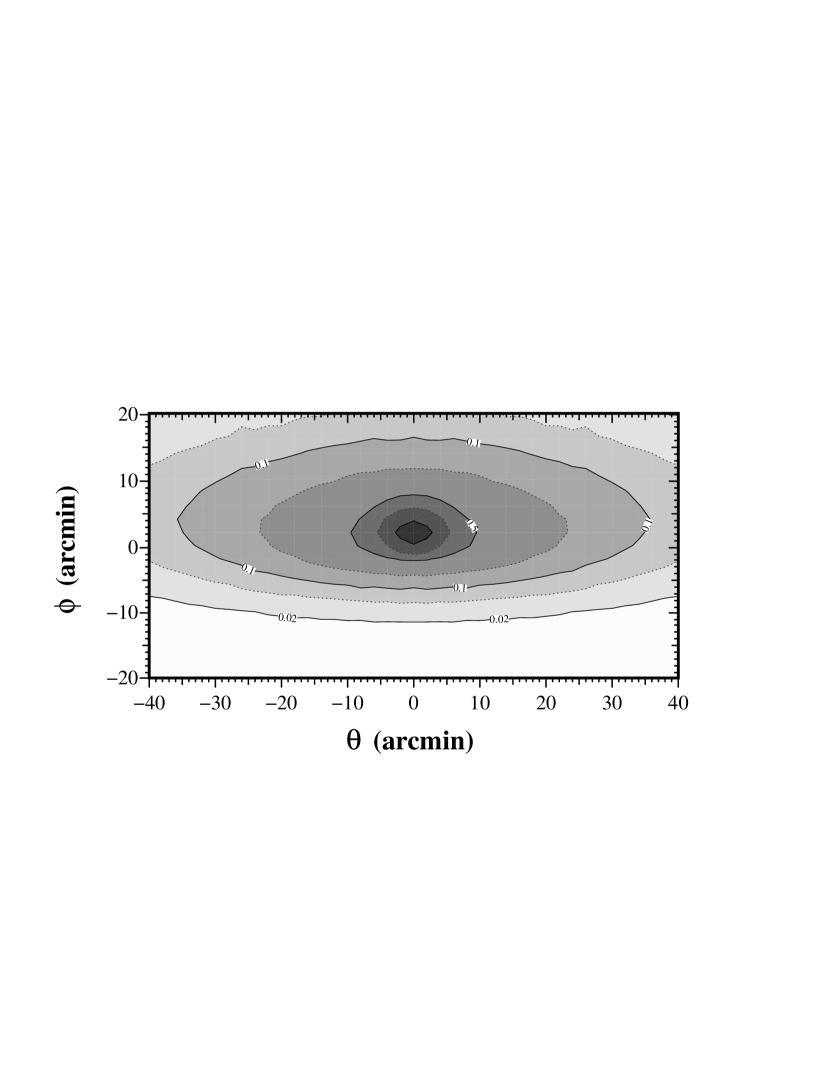
Figure 14: Contours of concurrent microlensing events per arcmin² for Model A assuming an all MACHO halo. Contours are, from the outside in, 0.02, 0.05, .1, .2, .5 1.0, 2.0.

The map of the number of concurrent events per arcmin² for Model A is shown in Figure 14.

The differential event rate (number of events per unit time as a function of duration and position across the M31 disk) may be calculated in a similar manner. A semi-analytic calculation, on the other hand, involves multidimensional integrals which may be prohibitively complicated depending on the functional form of the DFs.

7 Summary and Conclusions

The models for M31 presented in this paper are dynamically self-consistent, consistent with published observations, and stable against the rapid growth of bar-like modes in the disk. To the best of our knowledge, no other model of a disk galaxy satisfies these three criteria to the extent considered in this paper. Although KD constructed models for the Milky-Way that are dynamically self-consistent, stable, and have roughly the correct rotation curve, they did not attempt to fit their model to other types of data such as the surface brightness profile.

Our models span a wide range in halo size and shape. The most successful models assume a bulge mass that is nearly a factor of two smaller than the oft-quoted value from Kent (1989). Our galaxy model with $M_{b}=2.5\times 10^{10}\,M_{\odot}$ and $M_{d}=7\times 10^{10}\,M_{\odot}$ provides a good overall fit to observational data, yields mass-to-light ratios that are quite acceptable, and appears to be stable against bar formation. This disruptive bar instability becomes more apparent in the models with more massive disks, such as the model proposed by Kent (1989). At the other extreme lies the model of Kerins et al. (2001), having $M_{b}=4\times 10^{10}\,M_{\odot}$ and $M_{d}=3\times 10^{10}\,M_{\odot}$. Although their model is extremely stable against bar formation and reproduces the surface brightness profile nicely within the disk-bulge transition zone, the M31 rotation curve and inner velocity dispersion profile it provides do not fit the data at all well.

The favored model in our study is found to yield a poor match of the estimated baryon fraction with cosmological predictions, and it falls somewhat short of the total galaxy mass at large radii as determined from observations of dynamical tracers. Forcing a larger tidal radius ($R_{t}\sim 160$ kpc) improves these at the cost of the rotation curve fit. We attribute this failure to the form of the lowered Evans halo DF utilized in the KD algorithm, and propose the use of a halo DF that falls off more gradually with radius. A preliminary analysis suggests that if the halo of Model A is replaced by an appropriate NFW profile, the cosmological constraints are satisfied while the quality of the fit to the observational data is maintained.

Several improvements in the models are possible. For example, one can incorporate additional components of the galaxy such as a central black hole, thick disk, and stellar halo. The most serious drawback of the models is that they are axisymmetric and therefore cannot capture important aspects of M31 such as spiral structure and triaxiality of the bulge. Our models can serve as a starting point for investigations of these phenomena. In particular, models with $M_{d}\simeq 7\times 10^{10}\,{\rm M_{\odot}}$ will be studies using numerical simulations to see if we can produce spiral structure and a barlike bulge similar to what is observed in M31.

The methods described in this paper are completely general. When additional data become available, the algorithm can be rerun to determine a new suite of best-fit models. One extension that is soon to be implemented is the inclusion of a distribution of test-particles that are designed to represent a population of dynamical tracers such as globular clusters or satellite galaxies. In principle, the additional information from observations of these populations can constrain the extent and shape of the halo.

Appendix A KD model parameters

The input parameters for the KD algorithm are provided in Table 4 for the models presented in this paper. The parameters are as discussed in the text. The unit of length is $1\,{\rm kpc}$ and the unit of velocity is $100\,{\rm km\,s^{-1}}$. We set $G_{\rm newt}=1$, as is the convention in N-body simulations. This implies of unit of mass of $2.325\times 10^{-9}\,M_{\odot}$.

Table 1: Models with $q=1$ and $R_{t}$ unconstrained

Model	$M_{d}$	$M_{b}$	$\chi^{2}$	$\left(M/L_{R}\right)_{d}$	$\left(M/L_{R}\right)_{b}$	$M_{30}$	$M_{h}$	$R_{t}$
	($10^{10}\,M_{\odot}$)	($10^{10}\,M_{\odot}$)				($10^{10}\,M_{\odot}$)	($10^{10}\,M_{\odot}$)	(kpc)
A	7	2.5	0.70	4.4	2.7	36	32	80
B	7	1	2.29	4.5	1.3	38	27	38
C	7	4	1.55	4.4	4.1	29	33	129
D	14	2	0.63	8.6	2.4	32	32	201
K1	16	4	1.75	9.9	4.8	28	6.5	137
K2	3	4	1.28	2.0	3.2	50	120	155

Table 2: Models with $M_{d}=7\times 10^{10}\,M_{\odot}$, $M_{b}=2.5\times 10^{10}\,M_{\odot}$, and $q=1$

Model	$R_{t}$	$\chi^{2}$	$M_{h}$	$c$	$R_{200}$	$M_{200}$	$f_{B}$	$f_{B,NFW}$
	(kpc)		($10^{10}\,M_{\odot}$)		(kpc)	($10^{10}\,M_{\odot}$)
A	80	0.70	32	11.5	224	130	0.23	0.07
E	160	1.30	67	7.9	193	81	0.13	0.10

Table 3: Models with $M_{d}=7\times 10^{10}\,M_{\odot}$, $M_{b}=2.5\times 10^{10}\,M_{\odot}$, and $R_{t}$ unconstrained

Model	$q$	$\chi^{2}$	$R_{t}$ (kpc)	$M_{h}$ ($10^{10}\,M_{\odot}$)	$q_{h}$
A	1.00	0.70	80	32	0.93
Q1	0.85	0.63	37	17	0.59
Q2	0.85	1.08	58	23	0.61

Table 4: Input KD parameters for models in Tables 1, 2, and 3.

Model	$\Psi_{0}$	$\sigma_{0}$	$q$	$(\frac{r_{c}}{r_{K}})^{2}$	$R_{a}$	$m_{disk}$	$\rho_{b}$	$\Psi_{c}$	$\sigma_{b}$	$S_{b}$
A	-28.87	4.20	1.00	0.43	4.77	30.11	6.68	-16.26	2.24	0.80
B	-24.52	4.27	1.00	0.41	4.73	30.11	7.07	-18.55	2.24	0.85
C	-32.29	4.34	1.00	0.40	5.14	30.11	6.52	-14.79	2.41	0.81
D	-29.77	3.37	1.00	0.42	4.50	60.22	6.87	-17.96	2.05	0.77
E	-28.98	3.68	1.00	0.40	6.03	30.11	7.35	-16.68	2.26	0.81
K1	-34.86	3.58	1.00	0.43	4.30	68.82	6.38	-16.03	2.44	0.75
K2	-35.21	3.62	1.00	0.15	5.26	12.90	4.94	-17.90	1.62	0.82
Q1	-26.57	4.05	0.85	0.42	3.63	30.11	9.70	-13.81	2.57	0.80
Q2	-26.23	3.79	0.85	0.44	4.27	30.11	10.18	-13.74	2.55	0.80

Figure 1: The disk rotation curve. The rotation measurements of Kent (1989, “K89”) and Braun (1991, “B91”) are shown in the upper panel, and the smoothed rotation profile used in the model fitting is provided in the lower panel.

Figure 2: Bulge rotation velocity as a function of radius. The upper panel shows the bulge rotation measurements of McElroy (1983) for the north-east (NE) and southwest (SW) sides of the minor axis along an axis with a position angle of $45^{\circ}$. The smoothed bulge rotation curve data and errors used in the model fitting are shown in the lower panel.

Figure 3: Velocity dispersion measurements of McElroy (1983) along the major axis (upper-left panel) and minor axis (upper-right panel) of the bulge. The corresponding smoothed profiles used in the model fitting are shown in the lower panels. The four outer points in the minor axis data were neglected due to their large uncertainties.

Figure 4: Comparison of theoretical fits with observational data for Model A from Table 1. The upper left-hand panel shows the net rotation curve for the galaxy (solid line), along with the profiles for the individual components: bulge (dotted line), disk (dashed line) and halo (long-dashed line). The data points and error bars are those of the smoothed rotation profile given in Figure 1. The lower left-hand panel shows the surface brightness profile measurements with the model fits of the bulge (dotted line), disk (dashed line) and total light (solid line). The upper-right panel provides the bulge velocity profile data and model fit. The middle- and lower-right panels show the inner velocity dispersion data and resulting fits along the galaxy’s major and minor axes, respectively.

Figure 5: Comparison of theoretical fits with observational data for Model D (see Table 1). The plots and line types are as described previously in Figure 4.

Figure 6: Results of N-body simulations for Models A and D after several dynamical times. Upper panels provide face-on views of the disk for Model A (left) and Model D (right). Lower panels show the corresponding “observer’s view” with the disk tilted to an inclination angle $77^{\circ}$.

Figure 7: Comparison of theoretical fits with observational data for Model K1 (Kent, 1989, see Table 1). The plots and line types are as described previously in Figure 4.

Figure 8: Comparison of theoretical fits with observational data for Model K2 (Values for $M_{b}$ and $M_{d}$ from Kerins et al. (2001). See Table  1). The plots and line types are as described previously in Figure 4.

Figure 9: Comparison of the rotation curves for Models A and E (see Table 2).

Figure 10: Mass distribution for models of Table 2. Plotted is the total mass interior to the radius $r$ for Model A (solid line), Model E (dotted line), and modified Model A with an NFW halo (dashed line). Also shown are published mass estimates from studies of dynamical tracers: globular cluster data from Perrett et al. (2002, open triangle), Evans & Wilkinson (2000, open circle), and Federici et al. (1993, open square); satellite data from Côté et al. (2000, filled triangle), Evans et al. (2000, filled pentagon), Evans & Wilkinson (2000, filled circle), and Courteau & van den Bergh (1999, filled square); planetary nebula data from Evans & Wilkinson (2000, cross).

Figure 11: Line-of-sight velocity dispersion as a function of projected radius $s$. Solid line refers to Model A; Dotted line refers to Model E.

Figure 12: Comparison of the halo used in Model A with a closely matched NFW halo. Top panel - density profile; Middle panel - mass distribution; Bottom panel - halo contribution to the rotation curve. Solid lines refer to Model A; dashed lines refer to the NFW halo.

Figure 13: Comparison of the rotation curves for Models A, Q1 and Q2 (see Table 3).

References

- Alcock et al. (2000) Alcock, C., et al. 2000, ApJ, 542, 281
- Armaud & Evrard (1999) Armaud, M., & Evrard, A. E. 1999, MNRAS, 305, 631
- Bahcall & Tremaine (1981) Bahcall, J. N., & Tremaine, S. 1981, ApJ, 244, 805
- Baltz, Gyuk & Crotts (2002) Baltz, E. A., Gyuk, G., & Crotts, A. 2002, astro-ph/0201054
- Barnes & Efstathiou (1987) Barnes, J., & Efstathiou, G. 1987, ApJ, 319, 575
- Bell & de Jong (2001) Bell, E. F., & de Jong, R. S. 2001, ApJ, 550, 212
- Binney & Merrifield (1998) Binney, J., & Merrifield, M. 1998, Galactic Astronomy, Princeton Univ. Press, Princeton
- Binney & Tremaine (1987) Binney, J., & Tremaine, S. 1987, Galactic Dynamics, Princeton Univ. Press, Princeton
- Braun (1991) Braun, R. 1991, ApJ, 372, 54
- Bullock et al. (2001) Bullock, J. S., Kolatt, T. S., Sigad, Y., Somerville, R. S., Kravtsov, A. V., Klypin, A. A., Primack, J. R., & Dekel, A. 2001, MNRAS, 321, 559
- Burles, Nollett, & Turner (2001) Burles, S., Nollett, K. N., & Turner, M. S. 2001, ApJ, 552, L1
- Byrd (1978) Byrd, G. G. 1978, ApJ, 226, 70
- Calchi Novati et al. (2002) Calchi Novati, S., et al. 2002, A&A, 381, 848
- Côté et al. (2000) Côté, P., Mateo, M., Sargent, W. L. W., & Olszewski, E. W. 2000, ApJ, 537, L91
- Courteau & van den Bergh (1999) Courteau, S., & van den Bergh, S. 1999, AJ, 118, 337
- Cram, Roberts & Whitehurst (1980) Cram, T. R., Roberts, M. S., & Whitehurst, R. N. 1980, A&AS, 40, 215
- Crotts (1992) Crotts, A. P. S. 1992, ApJ, 399, L43
- Crotts & Tomaney (1996) Crotts, A., & Tomaney, A. 1996, ApJ, 473, L87
- Crotts et al. (2001) Crotts, A., Uglesich, R., Gould, A., Gyuk, G., Sackett, P., Kuijken, K., Sutherland, W., & Widrow, L. 2000 in Microlensing 2000: A New Era of Microlensing Astrophysics, ASP Conf. Proc. 239, ed. J. W. Menzies & P. D. Sackett
- de Bernardis et al. (2002) de Bernardis, P., et al. 2002, ApJ, 564, 559
- Deharveng & Pellet (1975) Deharveng, J. M., & Pellet, A. 1975, A&A, 38, 15
- Dehnen (2002) Dehnen, W. 2002, J. Comp. Phys., 179, 27
- Dubinski (1994) Dubinski, J. 1994, ApJ, 431, 617
- Evans (1993) Evans, N. W. 1993, MNRAS, 260, 191
- Evans & Wilkinson (2000) Evans, N. W., & Wilkinson, M. I. 2000, MNRAS, 316, 929
- Evans et al. (2000) Evans, N. W., Wilkinson, M. I., Guhathakurta, P., Grebel, E. K., & Vogt, S. S. 2000, ApJ, 540, L9
- Evans et al. (2002) Evans, N. W., Wilkinson, M. I., Perrett, K. M., & Bridges, T. J. 2002, ApJ, in press
- Federici et al. (1993) Federici, L., Bònoli, F., Ciotti, L., Fusi-Pecci, F., Marano, B., Lipovetsky, V. A., Niezvestny, S. I., & Spassova, N. 1993, A&A, 274, 87
- Gerhard (1986) Gerhard, O. E. 1986, MNRAS, 219, 373
- Gottesman & Davies (1970) Gottesman, S. T., & Davies, R. D. 1970, MNRAS, 149, 263
- Gyuk & Crotts (2000) Gyuk, G., & Crotts, A. 2000, ApJ, 535, 621
- Heisler, Tremaine & Bahcall (1985) Heisler, J., Tremaine, S., & Bahcall, J. N. 1985, ApJ, 298, 8
- Héraudeau & Simien (1997) Héraudeau, P., & Simien, F. 1997, A&A, 326, 897
- Hodge & Kennicutt (1982) Hodge, P. W., & Kennicutt, R. C. 1982, AJ, 87, 264
- Hohl (1971) Hohl, F. 1971, ApJ, 168, 343
- Kent (1989) Kent, S. 1989, PASP, 101, 489
- Kerins et al. (2001) Kerins, E., et al. 2001, MNRAS, 323, 13
- King (1966) King, I. R. 1966, AJ, 71, 64
- Kuijken & Dubinski (1994) Kuijken, K., & Dubinski, J. 1994, MNRAS, 269, 13
- Kuijken & Dubinski (1995) Kuijken, K., & Dubinski, J. 1995, MNRAS, 277, 1341 (KD)
- Lokas & Mamon (2000) Lokas, E. L., & Mamon, G. A. 2000, MNRAS, 321, 155
- Lasserre et al. (2000) Lasserre, T. et al. (2000), A&A, 355, L39
- Mateo (1998) Mateo, M. 1998, ARA&A, 36, 435
- McElroy (1983) McElroy, D. B. 1983, ApJ, 270, 485
- McGaugh (2001) McGaugh, S. 2001, astro-ph/0112357
- McGaugh et al. (2000) McGaugh, S. S., Schombert, J. M., Bothun, G. D., & de Blok, W. J. G. 2000, ApJ, 533, L99
- Navarro, Frenk & White (1996) Navarro, J. F., Frenk, C. S., & White, S. D. M. 1996, ApJ, 462, 563
- Nolthenius & Ford (1987) Nolthenius, R., & Ford, H. C., 1987, ApJ, 317, 62
- Ostriker & Peebles (1973) Ostriker, J. P., & Peebles, P. J. E. 1973, ApJ, 186, 467
- Perrett et al. (2002) Perrett, K. M., Bridges, T. J., Hanes, D. A., Irwin, M. J., Brodie, J. P., Carter, D., Huchra, J. P., & Watson, F. G. 2002, AJ, 123, 2490
- Press et al. (1986) Press, W. H., Flannery, B. P., Teukolksy, S. A., & Vetterling, W. T. 1986, Numerical Recipes, (Cambridge: Cambridge University Press)
- Rubin & Ford (1970) Rubin, V. C., & Ford, W. K. 1970, ApJ, 159, 379
- Rubin & Ford (1971) Rubin, V. C., & Ford, W. K. 1971, ApJ, 170, 25
- Sato & Sawa (1986) Sato, N. R., & Sawa, T. 1986, PASJ, 38, 63
- Sellwood (1985) Sellwood, J. A. 1985, MNRAS, 217, 127
- Stark (1977) Stark, A. A. 1977, ApJ, 213, 368.
- Tully & Fisher (1977) Tully, R. B. & Fisher, J. R. 1977, A&A, 54, 661
- Walterbos & Kennicutt (1987) Walterbos, R. A. M., & Kennicutt, R. C. 1987, A&AS, 69, 311
- Walterbos & Kennicutt (1988) Walterbos, R. A. M., & Kennicutt, R. C. 1988, A&A, 198, 61
- Warren et al. (1992) Warren, M. S., Quinn, P. J., Salmon, J. K., & Zurek, W. H. 1992, ApJ, 399, 405
- Widrow (2000) Widrow, L. M. 2000, ApJS, 131, 39
- Zhao (1997) Zhao, H. 1997, 287, 525