On Tripolar Magnetic Reconnection and Coronal Heating

Abstract

Using recent data for the photosphere-chromosphere region of the solar atmosphere the magnetic reconnection in tripolar geometry has been investigated through the procedure of Sturrock (1999). Particular attention has been given to the width of the reconnecting region, wave number of the rapidly growing tearing mode, island length scales, frequency of MHD fluctuations, tearing mode growth rate, energy dissipation rate and minimum magnetic field strength required to heat chromospheric plasma to coronal temperatures. It is found that small length scales are formed in the upper chromosphere. The maximum growth rate of tearing mode instability coincides with the peak in the energy dissipation rate both of which occur in the upper chromosphere at the same height. It is realized that the distribution of magnetic field with height is essential for a better understanding of the coronal heating problem.

Subject headings: Sun: chromosphere - Sun: corona - Sun: magnetic field

1 INTRODUCTION

Recently (Aschwanden, 2001) has used Yohkoh, Solar Heliospheric Observatory (SOHO) and Transition Region And Coronal Explorer (TRACE) observations in the evaluation of coronal heating models for active regions. He focusses on three main results obtained from aforesaid spacecrafts, namely, the overdensity of coronal loops, chromospheric upflows of heated plasma and the localization of heating in the lower corona. He examines various A.C. and D.C. models on the basis of above criteria. In D.C. models he considers bipolar, tripolar and quadrupolar magnetic reconnection and favours tripolar magnetic reconnection where magnetic reconnection between two polarities of a closed and the unipolar footpoint of an open field line may take place. Such a situation may arise due the emergence of a new dipole in an open field region or by the collision of the footpoint of an open field line with an adjacent dipole. In this case the open field line can carry hot plasma upward into the upper corona, regardless of the size of the interacting dipole. Thus tripolar reconnection is highly relevant for the coronal heating especially for open field regions such as coronal holes.

(Chae et al., 2000) have studied transient network brightenings (blinkers) and explosive events in the solar transition region, recorded by the Coronal Diagnostic Spectrometer (CDS) in the line O V $\lambda$ 630 and Solar Ultraviolet Measurements of Emitted Radiation (SUMER) instrument in the line Si IV $\lambda$ 1402 together with the photospheric magnetograms taken by the Big Bear Solar Observatory videomagnetograph. They find that the explosive events (which are features with very broad UV line profile) tend to keep away from the centres of network brightenings. CDS blinkers contain many small-scale short-lived SUMER ‘unit brightening events’ having size of a few arc seconds and a lifetime of a few minutes. Each of these unit brightening events is characterized by a UV line profile which is not as broad as those of explosive events. Thus blinkers (transient network brightenings) and explosive events both may be due to magnetic reconnection with different geometries.

The explosive events are considered to occur as a result of the collision of a network flux thread (which is part of a very large loop) and an intranetwork flux thread which is part of a very small loop ( Chae et al. (1999), Chae et al. (2000) ). This interaction has therefore the potential for conveying hot plasma into large- scale loops and is a very suitable mechanism for explaining the observed footpoint heating, upflows and overdensity in EUV loops. Further, the relaxation of the newly formed open field line may accelerate acoustic waves or shock waves and heat plasma along its passage. Thus the process of tripolar magnetic reconnection has a better connectivity to the upper corona and to the solar wind via the open field line than bipolar and quadrupolar reconnection geometries (Aschwanden, 2001).

When two open magnetic field lines of opposite polarity reconnect, the newly configured polarities relax into two bipolar field lines. The lower one connects the two magnetically conjugate photospheric footpoints whereas the upper ends of the disconnected field lines in the upper corona combine and finally move into interplanetary space. Thus there is a high-density closed loop downward and a low-density segment moving upward (see, e.g., Shimizu et al. (1992); (Krucker & Benz, 2000); (Parnell & Jupp, 2000); Aschwanden et al. (2000) ). This type of heating process is applicable to big or small flares (including micro- and nano-flares) ((Parker, 1991); (Brown et al., 2000)). Bipolar magnetic reconnection has been investigated, in some way or other, by (Litvinenko, 1999) , (Longcope & Kankelborg, 1999) , (Furusawa & Sakai, 2000) , Sakai et al. (2000) , (Sakai, Takahata,& Sokolov, 2001) also.

Quadrupolar magnetic reconnection has been observed and modeled in solar flares ( Uchida et al. (1994); (Uralov, 1996); (Hanaoka, 1996) ; Nishio et al. (1997); Aschwanden et al. (1999)). Here the exchange of connectivity between positive and negative polarities in a system with two closed field lines takes place by pushing them into physical contact such that the new configuration is in a lower energy state.

Chromospheric quadrupolar magnetic reconnection between two contiguous flux tubes of opposite polarity has been considered by (Sturrock, 1999) in connection with its possible relationship to coronal heating. His basic idea has been that reconnection occurs preferentially where the growth rate of the relevant instability is greatest. He arrives at the conclusion that quadrupolar magnetic reconnection can lead to coronal heating by Joule dissipation and by the generation and subsequent dissipation of high frequency Alfvén and magnetoacoustic waves. The heating of solar wind particles may take place when high frequency Alfvén waves, produced during reconnection, are absorbed by cyclotron damping.

In view of above it seems quite worthwhile to study magnetic reconnection in tripolar geometry such as that given in Fig. 1. In §2 we present the relevant theoretical details. The data used and the results obtained, exhibited in §3, are discussed in §4 alongwith our conclusions.

Throughout cgs system of units is used. Wherever necessary, the heights are expressed in km.

2 THEORETICAL DETAILS

We adopt the formalism of (Sturrock, 1999). As shown in Fig. 1 there is a network flux thread (part of a very large loop) which collides with an intranetwork flux thread which is a part of very small loop. It is assumed that magnetic reconnection would occur preferentially where the growth rate of resistive tearing mode instability is greatest. The medium under consideration is a partially ionized hydrogen plasma so that the role of helium and other elements may be ignored.

The tearing mode growth rate depends on the wave number of the mode. The wave number of the most rapidly growing mode is given by (Sturrock, 1994)

$$k_{M}=1.4R_{m}^{-0.25}l^{-1},$$ (1)

where $l$ is the width of the reconnecting region and $R_{m}$, the transverse magnetic Reynolds number, is given by

$$R_{m}=t_{D}/t_{A},$$ (2)

with

$$t_{D}=4{\pi}l^{2}/{\eta}c^{2},$$ (3)

and

$$t_{A}=l/v_{A}.$$ (4)

Here $t_{D}$ is the resistive diffusion time, $t_{A}$ the Alfvén transit time, $v_{A}$ the Alfvén velocity, c the speed of light in vacuum and $\eta$, the Coulomb resistivity of the hydrogenic plasma, is given by (Spitzer, 1962)

$$\eta=1.510^{-7}T^{-1.5}s$$ (5)

In equation (5), T is the temperature of the hydrogenic plasma. The Alfvén velocity $v_{A}$ is estimated through the following equation

$$v_{A}=B/(4\pi\rho)^{0.5},$$ (6)

where the mass density $\rho$ may be obtained from

$$\rho=(n_{p}+n_{H})m_{p}.$$ (7)

In the above B is the magnetic field strength before reconnection, $n_{p}$ and $n_{H}$ are the number densities of proton and neutral hydrogen, respectively.

The growth time $t_{g}$, which is the inverse of the growth rate, is given by

$$t_{g}=1.585R_{m}^{-0.5}t_{D}.$$ (8)

The growth rate of instability depends sensitively upon the assumed width $l$ of the current sheet between two flux tubes and it may be related to the pressure scale height H by

$$l={\epsilon}H.$$ (9)

Here $\epsilon$ is a dimensionless parameter and the scale height $H$ is given by

$$H=10^{3.48}Tm_{p}/m_{av},$$ (10)

with

$$m_{av}=(n_{p}+n_{H})m_{p}/(n_{e}+n_{p}+n_{H}),$$ (11)

where $m_{p}$ is the proton mass and $n_{e}$ the number density of electrons.

The tearing mode instability leads to the formation of small islands which allow for the rapid diffusion of the magnetic field. For the most rapidly growing mode the island length scale $x_{TM}$ is given by

$$x_{TM}=1.51R_{m}^{-0.25}l.$$ (12)

If the tearing region is in a dynamic state and the inhomogeneities move at the Alfvén speed then they will lead to fluctuations having frequency $\nu_{TM}$ given by

$$\nu_{TM}=v_{A}/x_{TM}.$$ (13)

Such fluctuations may play a role in providing additional thermal energy to the corona.

The average energy dissipation rate in the reconnection region may be obtained from(Tandberg-Hanssen & Emslie 1988)

$$U_{t}=B^{2}V/8{\pi}t_{R},$$ (14)

where $V$ is the volume of the reconnecting region(s) and $t_{R}$, the reconnection time scale, is given by (Spicer, 1977)

$$t_{R}=t_{A}^{0.4}t_{D}^{0.6}.$$ (15)

In the case of multiple reconnecting regions, as in the tearing mode, the volume of reconnecting region may be taken to be $V=L^{2}l$, where L is the longitudinal length scale and $l$ is the width. As an approximation L may be taken to be the diameter of the flux tube.

It is possible to estimate the minimum strength of the magnetic field required to heat the reconnecting region to coronal temperature ($10^{6}$K) by using the following relation

$$1.5nk_{B}T=B_{min}^{2}/8{\pi},$$ (16)

where $k_{B}$ is the Boltzmann constant and n is given by

$$n=n_{e}+n_{p}+n_{H}.$$ (17)

Such an estimate can be made at each height where magnetic reconnection can occur.

3 THE DATA AND RESULTS

For the sake of completeness the data taken from Cox (2000) have been exhibited in Figures 2 and 3. In particular, Fig. 2 shows variation of temperature with height in the photosphere-chromosphere region whereas Fig. 3 exhibits $n_{e}$, $n_{p}$ and $n_{H}$ as a function of height h in km.

The data of Fig. 2 and equation (5) have been used to obtain resistivity $\eta$ as a function of height and is displayed in Fig. 4. Since the resistivity is inversely proportional to $T^{1.5}$ it has maximum value in the temperature minimum region.

The data of Figures 2 and 3 together with equations (10) and ( 11) lead to the results displayed in Fig. 5 where the scale height H is shown to vary with height in the lower solar atmosphere. The lowest value of scale height falls in the temperature minimum region.

In order to estimate the width $l$ of the reconnecting region we require the value of parameter $\epsilon$. This can be done by estimating the length over which the magnetic field will diffuse over a time scale characteristic of changes in the photosphere, e.g., the mean lifetime of photospheric granules which is 10 minutes ((Cox, 2000)). This procedure alongwith equations (3), (5), (9) and the data of Fig. 2 give $\epsilon=0.0114$ corresponding to $l=1.48$ km and $T=4400K$ at 520 km. Now equation (9) alongwith the results of Fig. 5 may be used to obtain the width $l$ of the reconnecting region as a function of height which is displayed in Fig. 6.

The nature of variation of width with height is similar to that of scale height vs height curve, as expected.

The evaluation of Alfvén transit time $t_{A}$ requires the values of Alfvén velocity $v_{A}$ and the width $l$. In order to determine $v_{A}$ we require the magnetic field strength as a function of height (which is not known) and the mass density $\rho$. Assuming a constant mean value $B=100$ G, the data of Fig. 3 and equation (7), the Alfvén velocity has been determined and is displayed in Fig. 7 as a function of height.

As expected $v_{A}$ increases with height because $\rho$ decreases with height. Using the values of $l$ and $v_{A}$ the Alfvén transit time becomes known through equation (4).

With the width $l$ and the resistivity $\eta$ known it is possible to determine resistive diffusion time $t_{D}$ by using equation (3). This enables us to find transverse magnetic Reynolds number $R_{m}$ through equation (2). The Reynolds magnetic number has been displayed in Fig. 8 as a function of height. The resulting curve shows a minimum near 100 km and increases upwards monotonically. The resistive diffusion time $t_{D}$ is displayed in Fig. 9 as a function of height.

Using equation (1), the values of $R_{m}$ and width $l$ it is possible to evaluate the wave number $k_{M}$ of the most rapidly growing mode. This wave number as a function of height is displayed in Fig. 10. It shows a broad maximum in the 0 - 700 km region.

The growth time (which is the inverse of growth rate) has been obtained through Equation (8) and the already known values of the magnetic Reynolds number (Fig. 8) and the resistive diffusion time (Fig. 9). The growth time $t_{g}$ and the growth rate are displayed in Figures 11 and 12, respectively.

The growth rate curve shows a maximum at 1800 km and the growth time curve shows a minimum at the same height, as it should.

Using Equation (15), the resistive diffusion time t_D and the Alfvén transit time t_A we obtained reconnection time t_R which is exhibited as a function of height in Fig. 13. It exhibits a broad minimum in the range 1200 - 1900 km. It appears that the reconnection is slower in the temperature region and faster in the upper chromosphere.

Fig. 14 exhibits island length scales $x_{TM}$ as a function of height. These values have been obtained from Equation (12), the magnetic Reynolds number (Fig. 8) and the width $l$ of the reconnecting region (Fig. 6).

The shortest length scales are obtained around 1900 km in the upper chromosphere which is a desirable feature for all coronal heating mechanisms (Aschwanden, 2001).
The frequencies of MHD waves generated as a result of fluctuations in the reconnecting region are displayed in Fig. 15. These frequencies increase from temperature minimum region to upper chromosphere, similar to (Sturrock, 1999), monotonically.

Using Equation (14), $B=100$ G, $L=10^{8}$ cm, the width $l$ (Fig. 6) of reconnecting region and reconnection time $t_{R}$ (Fig. 13) we estimate the average energy dissipation rate as a function of height. This result is displayed in Fig. 16 which shows that the energy dissipation rate increases with height upto 1800 km and falls upwards. . The peak in dissipation rate agrees with the peak in the growth rate of the tearing mode instability. The height of peak dissipation rate finds favour with the observation made by (Aschwanden, 2001).

In Fig. 17 we display the minimum magnetic field strength $B_{min}$ required to heat the reconnecting site to coronal temperatue $10^{6}K$ as a function of height. It is clear from this curve that at a height of 1600 km the required minimum magnetic field is about 100 G whereas at a height of 500 km it is about 6000 G. Such a possibility is consistent with the evidence for direct heating of chromospheric gas to coronal temperatures (Krucker & Benz, 1998).

4 DISCUSSION AND CONCLUSIONS

The data, namely, temperature $T$, electron, proton and hydrogen number densities $n_{e},n_{p},n_{H}$ and mean lifetime of granules, used by us are of quite recent origin and seem to be reliable. The temperature minimum occurs near 500 km (Fig. 1). At each height the number density of neutral hydrogen is greater than the number densities of electrons and protons (Fig. 3).

The classical Coulomb resistivity $\eta$ is inversely proportional to $T^{1.5}$ consequently it has largest value at that height at which the temperature is minimum. Similar trend is noticeable at other heights (Fig. 4).

The scale height $H$ and width $l$ of the reconnecting region vary with height in the same way. Both of them have their minimum values near 500 km. Essentially, the nature of curves of temperature, scale height, width, resistivity is quite similar, as expected.

Because of decreasing mass density $\rho$ the Alfvén velocity increases with height, monotonically as the magnetic field strength $B$ before reconnection has been given a fixed value of 100 G. For the better understanding of the coronal heating problem the distribution of magnetic field with height is quite essential.

The magnetic Reynolds number determines to what extent the field is frozen into the plasma. Higher values of $R_{m}$ means better frozen-in-field approximation. In the region under consideration $R_{m}$ varies from about $3\times 10^{3}$ to $3\times 10^{7}$, i.e. the frozen-in-field approximation is quite good to describe photospheric-chromospheric region (Fig. 8).

The resistive diffusion time $t_{D}$ varies with height (Fig.9) in the same way as the temperature. It has minimum value near 500 km and lies in the range $6\times 10^{2}s<t_{D}<6\times 10^{4}s$ for the solar atmospheric region under consideration.

The wave number of the rapidly growing mode shows a broad peak in the region 0 - 700 km (Fig. 10). This is because $k_{M}$ is inversely proportional to the width of reconnecting region which has minimum value in the aforesaid region.

The growth time of instability decreases monotonically with height upto 1900 km and increases upwards (Fig.11). Since the growth rate is the inverse of growth time hence growth rate exhibits opposite nature (Fig. 12). The growth rate is maximum at 1800 km consequently heating is expected to occur near this height. In fact, the energy dissipation rate is maximum at 1800 km (Fig. 16). Thus the growth rate seems to be a better indicator of heating. Further the magnetic reconnection time $t_{R}$ has minimum value in the 1200 - 1900 km region (Fig.13) but the width of the reconnecting region is larger in this region. Since the energy dissipation rate varies directly with width and inversely with reconnection time hence the above- mentioned behaviour of dissipation rate is quite expected.

It is clear from Fig. 14 that the island length scale has its lowest value at 1900 km. Since smaller length scales are more efficient in energy dissipation than larger length scales hence the above heating rate is in agreement with this well-known result.

The energy dissipation rate (Fig. 16) gets support from the minimum magnetic field strength vs height curve (Fig. 17) because at 1900 km the required minimum magnetic field strength $B_{min}$ to heat the chromospheric plasma to coronal temperature is about 100 G. It is this value which has been used to obtain Alfvén velocity $v_{A}$, Alfvén transit time $t_{A}$ etc. .

The frequency of MHD waves, generated due to magnetic reconnection, increases with height (Fig. 15). Since the higher frequency waves may dissipate more readily than the lower frequency waves hence the heating wil be enhanced by the high frequency waves higher up in the atmosphere. Similar conclusion has already been forwarded by (Sturrock, 1999).

In tripolar geometry (Fig. 1) a network flux thread which is a part of a very large loop collides with an intranetwork flux thread which is part of a very small loop. At the intersection point the two flux threads are antiparallel, forming a relative angle that is greater than 90 degree. Consequently the reconnection at the intersection point could produce strong bidirectional outflows (Fig. 1a). This explains explosive events showing high velocity motions in their line profiles.

The open field line may carry hot plasm upward into the upper corona, regardless of the size of the interacting dipole. The open field line may also act as a waveguide to send MHD fluctuations into the corona and interplanetary space.

Thus tripolar reconnection is a very suitable mechanism for heating open field regions (coronal holes) in particular and the solar corona in general. It may also accelerate the solar wind particles.

We are grateful to Professor J.V. Narlikar, Director for his kind hopitality, encouragement and all possible help during our stay at IUCAA, Pune. One of us (U.N.) is grateful to Meerut College authorities for granting duty leave during the course of this work. The help of Dr. Sudhanshu in computation and related problems is thankfully acknowledged. Thanks are due to Dr. Nagendra Kumar for carefully reading the manuscript.

Figure 1: Variation of temperature with height

Figure 2: Variation of electron, proton and hydrogen density with height

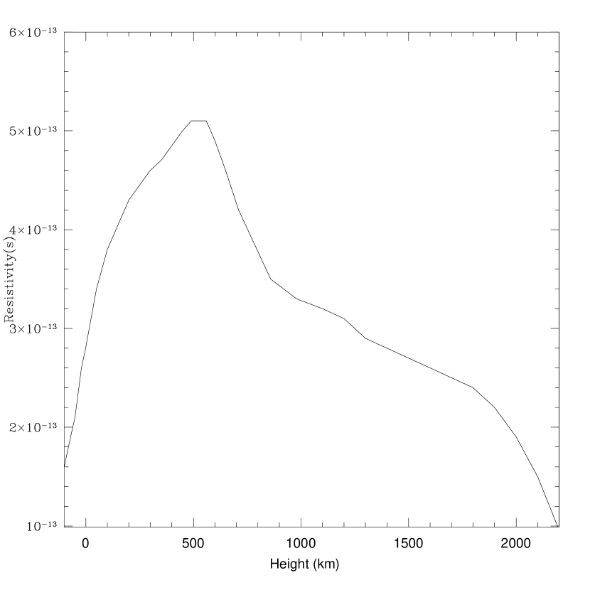
Figure 3: Variation of resistivity $\eta$ with height

Figure 4: Variation of temperature scale height H with height h

Figure 5: Variation of width of reconnecting region with height

Figure 6: Variation of Alfvén velocity with height

Figure 7: Variation of magnetic Reynolds number with height

Figure 8: Variation of resistive diffusion time with height

Figure 9: Variation of wave number of the most rapidly growing mode with height

Figure 10: Variation of tearing mode growth time with height

Figure 11: Variation of growth rate of the tearing mode with height

Figure 12: Variation of magnetic reconnection time with height

Figure 13: Variation of tearing mode scale length with height

Figure 14: Variation of fluctuation frequency with height

Figure 15: Variation of energy dissipation rate with height

Figure 16: Variation of required minimum magnetic field strength with height

References

- Aschwanden (2001) Aschwanden, M.J. 2001, ApJ, 560, 1035
- Aschwanden et al. (2000) Aschwanden, M.J., Tarbell, T., Nightingale, R.,Schrijver,C.J., Title, A., Kankelborg, C.C., Martens, P.C.H., & Warren, H.P. 2000, ApJ, 535, 1047
- Aschwanden et al. (1999) Aschwanden, M.J., Kosugi, T., Hanaoka, Y., Nishio, M., & Melrose, D.B. 1999, ApJ, 526, 1026
- Brown et al. (2000) Brown, J.C., Krucker, S., Guedel, M., & Benz, A.O. 2000, A&A, 359, 1185
- Chae et al. (2000) Chae, J.,Wang, H., Goode, P.R., Fludra, A., & Schuehle, U. 2000, ApJ, 528, L119
- Chae et al. (1999) Chae, J., Qiu, J., Wang, H., & Goode, P. 1999, ApJ, 513, L75
- Cox (2000) Cox, A.N. (ed.) 2000, Allen’s Astrophysical Quantities (Los Alamos: AIP Press), Chap. 14
- Furusawa & Sakai (2000) Furusawa, K.,& Sakai, J.I. 2000, ApJ, 540, 1156
- Hanaoka (1996) Hanaoka, Y. 1996, Sol. Phys., 165, 275
- Krucker & Benz (2000) Krucker, S. & Benz, A.O. 2000, Sol. Phys., 191, 341
- Krucker & Benz (1998) Krucker, S. & Benz, A.O. 1998, ApJ, 501, L213
- Litvinenko (1999) Litvinenko, Y.E. 1999, ApJ, 515, 435
- Longcope & Kankelborg (1999) Longcope, D.W., & Kankelborg, C.C. 1999, ApJ, 524, 483
- Nishio et al. (1997) Nishio, M., Yaji, K., Kosugi, T., Nakajima, H. & Sakurai, T. 1997, ApJ, 489, 976
- Parker (1991) Parker, E.N. 1991, in Mechanisms of Chromospheric and Coronal Heating, (ed.) P. Ulmschneider, E.R. Priest & R. Rosner (Berlin: Springer), 615
- Parnell & Jupp (2000) Parnell, C.E., & Jupp, P.E. 2000, ApJ, 529,554
- Sakai et al. (2000) Sakai, J.I, Kawata, T., Yoshida, K., Furusawa, K.,& Kramer, N.F. 2000, ApJ, 537, 1063
- Sakai, Takahata,& Sokolov (2001) Sakai, J.I., Takahata, A., & Sokolov, I.V. 2001, ApJ, 556, 905
- Shimizu et al. (1992) Shimizu, T., Tsuneta, S., Acton, L.W., Lemen, J.R., & Uchida, Y. 1992, PASJ, 44, L147
- Spicer (1977) Spicer, D.S. 1977, Sol. Phys., 53, 305
- Spitzer (1962) Spitzer, L. Physics of Fully Ionized Gases (New York: Interscience),
- Sturrock (1999) Sturrock, P.A. 1999, ApJ, 521, 451
- Sturrock (1994) Sturrock, P.A. 1994, Plasma Physics (New York:Cambridge Univ. Press), Chap. 17
- Tandberg-Hanssen & Emslie (1988) Tandberg-Hanssen, E. & Emslie, A.G. 1988, The Physics of Solar Flares (New York: Cambridge Univ. Press), Chap. 7
- Uchida et al. (1994) Uchida, Y., McAllister, A., Khan, J., Sakurai, T., & Jockers, K. 1994, in X-ray Solar Physics from Yohkoh, ed. Y. Uchida, T. Watanabe, K. Shibata & H.S. Hudson (Tokyo: Universal Academy Press), 161
- Uralov (1996) Uralov, A.M. 1996, Sol. Phys., 168, 311