A Fourier-Based Algorithm for Modelling Aberrations in HETE-2’s Imaging System

Abstract

The High-Energy Transient Explorer (HETE-2), launched in October 2000, is a satellite experiment dedicated to the study of $\gamma$-ray bursts in a very wide energy range from soft X-ray to $\gamma$-ray wavelengths. The intermediate X-ray range (2-30 keV) is covered by the Wide-field X-ray Monitor WXM, a coded aperture imager. In this article, an algorithm for reconstructing the positions of $\gamma$-ray bursts is described, which is capable of correcting systematic aberrations to approximately $1^{\prime}$ throughout the field of view. Functionality and performance of this algorithm have been validated using data from Monte Carlo simulations as well as from astrometric observations of the X-ray source Scorpius X-1.

,

Introduction

Although the number of detected $\gamma$-ray bursts has increased tremendously due to the BATSE instrument on board the Compton $\gamma$-Ray Observatory [1], unique identifications and quick follow-up observations of the celestial object that harbours the burst site are rare. This issue has been successfully addressed by the BeppoSAX satellite, that monitors a large fraction of the sky ($\sim 1\mbox{ sr}$) in the intermediate X-ray range [2, 3] and is able to derive burst localisations with an accuracy of $\sim 1^{\prime}$. With such improved localisations, the Beppo-SAX team has succeeded in detecting X-ray afterglows [4], by which valuable insight into the emission mechanism was gained. Finding $\gamma$-ray burst counterparts and performing spectroscopy at wavelengths other than the $\gamma$-ray band during the active phase of a burst as well as providing good localisations for follow-up observations is the basic scientific motivation of the HETE-2 mission.

This publication is structured as follows: After a brief description of HETE-2’s instrumentation in section 1, the position reconstruction algorithm is outlined in section 2. The performance of the algorithm on Monte Carlo generated events as well as on data taken in astrometric observations of the X-ray source Scorpius X-1 is presented in section 3. In section 4 findings on the point spread function are shown. A summary in section 5 concludes the paper.

1 HETE-2 Mission

The High Energy Transient Explorer (HETE-2) is a dedicated mission for the localisation and spectroscopy of $\gamma$-ray bursts. Details of the instrumentation of HETE-2 and the mission are given in [5]. Its scientific payload consists of three experiments: FREGATE, a scintillation crystal experiment, that is expected to provide triggers because of its high sensitivity and large sky coverage, SXC, a coded-mask imager based on a X-ray CCD chip design, which is able to localise $\gamma$-ray bursts with very high spatial resolution, and the core experiment WXM.

The Wide Field X-ray Monitor WXM consists of two perpendicularly oriented 1-dimensional coded mask cameras, in which photons are detected by position sensitive proportional counters. The detectors, one pair for each of the two orthogonal systems, are filled with xenon gas at a pressure of $1.4\mbox{ bar}$ with an admixture of $3\%$ carbon dioxide as a quenching gas. Each detector contains three carbon wire anodes in which the position of an absorbed photon is inferred by comparing the accumulated charges at both ends of a wire. WXM achieves a position resolution of $1\mbox{ mm}$ (FWHM) at $6\mbox{ keV}$. A veto system below the counting wires reduces the background due to charged particles. WXM is sensitive to photons with energies $E$ in the range $2\mbox{ keV}\leq E\leq 30\mbox{ keV}$ with an relative energy resolution of $\Delta E/E=8\%$ at $E=8\mbox{ keV}$.

The mask pattern, identical for the $x$- and $y$-system, is placed $d=187\mbox{ mm}$ above the detectors and is composed of 103 elements, each $2\mbox{ mm}$ in width. On third of the elements are open and randomly distributed. The parameters have been optimised with respect to source localisation accuracy for the expected levels of signal and background photon count rates [6]. The combined $x$- and $y$-systems are monitoring a field of view of approximately $60^{\circ}\times 60^{\circ}$. Figure 1 shows the actual mask pattern of a WXM camera. Further details of the WXM cameras can be found in [yuji].

Figure 1: The coded mask of HETE-2’s wide-field X-ray monitor WXM

In order to provide other experiments with precise localisations of $\gamma$-ray burst sites within seconds after burst onset, an array of twelve burst alert stations has been installed below HETE-2’s flight path. Once received, the information is relayed to the GRB Coordinate Network (GCN), from where it may be obtained by interested observers.

2 Position Reconstruction Algorithm

For the sake of readability, the algorithm is described for determining the angle of incidence $\theta_{x}$ in the $x$-detector, completely analogous formulae apply to the $y$-system. Figure 2 provides the definition of all quantities involved.

Figure 2: The definition of geometrical quantities in the WXM coordinate system.

2.1 Correlation

The task of localising a single point source is performed by computing the correlation function $\left[f\otimes m\right](x)$ of the mask pattern $m(x)$ and the recorded intensity distribution $f(x)$; the asterisk denoting complex conjugation:

$$\left[f\otimes m\right](x)=\int m(\lambda)\cdot f^{*}(\lambda+x)d\lambda\mbox{.}$$ (1)

The correlation function $[f\otimes m](x)$ will peak at a value $x_{0}$, indicating the distance $f(x)$ is shifted with respect to $m(x)$. This yields the angle of incidence $\theta_{x}$ by $\tan\theta_{x}=x_{0}/d$, where $d=187\mbox{ mm}$ is the distance between mask and detector. In $m(x)$, open elements of the mask pattern have been assigned a value of $1$, whereas closed elements correspond to a value of $\tau/(\tau-1)=-1/2$, where $\tau=1/3$ is the open fraction of HETE-2’s imaging system. This method is known as balanced correlation and removes the correlation background.

There exist more sophisticated correlation schemes such as unbiased balanced correlation (e.g. [9], [10]), that do take into account partial shadowing of the mask onto the detector by bursts in the periphery of the field of view and increased coding noise caused by steady strong off-axis sources. For HETE-2’s flight algorithm we rely on basic balanced correlation for three reasons: The width of the mask is almost twice as large as the active area of the detector and only bursts at angles $\geq 25^{\circ}$ off the optical axis are affected by partial shadowing. Furthermore, the running average of the mask’s transparency is close to constant with deviations being very small, so that the modulation of the pattern is insensitive to angle of incidence. Thirdly, in HETE-2’s nominal survey mode, the satellite is rotated in such a way that strong X-ray sources are avoided and the assumption of isotropically incidenting background radiation is valid.

2.2 Imaging Aberrations

In reality the correlation is complicated by imperfections of the detector: The photons travel a finite path before interacting and the loci of photons interacting in the detector are measured with finite position resolution (in the case of WXM to $1\mbox{ mm}$, subtending an angle of $18^{\prime}$). Whereas the finite position resolution simply results in a blurring of the image, the penetration of energetic photons effectively induces an additional shift in the image, if the event is happening at nonzero angles of incidence, and causes the angles of incidence to be overestimated. This effect increases in a complex fashion with distance from the center of the field of view and is of the order of $12^{\prime}$ at $30^{\circ}$ from the optical axis for a photon distribution following a power law spectrum with a spectral index of $\Gamma=1.1$.

In contrast to a time consuming Monte Carlo simulation, in which one determines the image of the mask pattern under estimated angles of incidence, the algorithm presented in this article aims at modelling all effects involved in the delapidation of the mask pattern, enabling a much faster localisation of the $\gamma$-ray burst site.

2.3 Convolutions

Imaging aberrations may be described by applying suitable changes to the mask pattern $m(x)$ prior to the calculation of the correlation function. This can be archieved by convolving the mask pattern $m(x)$ with integration kernels $p(x)$ and $r(x)$, that describe the penetration of highly energetic photons and the detector resolution, respectively,

$$\left[p\odot m\right](x)=\int m(\lambda)\cdot p(x-\lambda)d\lambda\mbox{.}$$ (2)

The convolution kernel $p(x)$ that is used for describing the penetration of photons is given by equation 3:

$$p(x)=\frac{1}{a_{\|}(\theta_{x},\theta_{y})}\exp\left(-\frac{x}{a_{\|}(\theta_{x},\theta_{y})}\right)\cdot\Theta\left(\mbox{\em sgn}\left[\theta_{x}\right]\cdot x\right)\mbox{,}$$ (3)

where $\Theta$ is the Heaviside function and sgn the signum function The convolution yields an altered mask pattern $m^{\prime}(x)=[p\odot m](x)$, in which the penetration of photons is incorporated. The length scale $a_{\|}$ of the exponential decay, given by equation 4, is equal to the spectrally averaged attenuation length $a$ of photons inside the detector, corrected by a projection factor:

$$a_{\|}(\theta_{x},\theta_{y})=a\cdot\frac{\tan\theta_{x}}{\sqrt{1+\tan^{2}\theta_{x}+\tan^{2}\theta_{y}}}\mbox{.}$$ (4)

Estimates for the angles of incidence $\theta_{x}$ and $\theta_{y}$ follow from a source localisation with the unmodified mask pattern $m(x)$ in a first step. The finite spatial resolution of the position sensitive proportional counter is described by convolution with a Gaussian integration kernel as in equation 5:

$$r(x)=\frac{1}{\sqrt{2\pi}c}\exp\left(-\frac{x^{2}}{2c^{2}}\right)\mbox{ with }c=1/\sqrt{8\cdot\ln 2}\mbox{ mm.}$$ (5)

The standard deviation corresponds to a value for full width half maximum of $1\mbox{ mm}$. In contrast to $a$, $c$ depends only very weakly on the spectral distribution of the incident photons and is considered to be constant. After convolution with $r(x)$, the mask pattern has been modified to $m^{\prime\prime}(x)=[r\odot m^{\prime}](x)$. $m^{\prime\prime}(x)$ is the image of the mask pattern under ideal statistics and the source reconstruction with $m^{\prime\prime}(x)$ should not display any deviation from the ideal behaviour. The correlation $[f\otimes m^{\prime\prime}](x)$ yields a corrected value $\theta_{x}^{\prime}$ for the angle of incidence.

2.4 Correlation in Fourier Space

Due to their high numerical complexity it is favourable to perform both the convolutions and the image localisation by correlation in the Fourier domain. The nomenclature is such that lower case letters denote functions in real space and the corresponding upper case letters their Fourier transforms:

$$M(k)=\mathcal{F}\left[m(x)\right]=\frac{1}{2\pi}\int m(x)\exp(-ikx)dx\mbox{.}$$ (6)

Convolutions and correlations reduce by virtue of equation 7 to mere multiplications in Fourier space. The asterisk denotes complex conjugation:

$$\begin{array}[]{lcl}\left[p\odot m\right](x)&=&\mathcal{F}^{-1}\left[P(k)M(k)\right]\mbox{,}\\ \left[f\otimes m^{\prime\prime}\right](x)&=&\mathcal{F}^{-1}\left[F(k)^{*}M^{\prime\prime}(k)\right]\mbox{.}\end{array}$$ (7)

Diagram 8 summarises all steps. Starting from the Fourier-transform of the mask pattern $M(k)=\mathcal{F}[m(x)]$, both convolutions and the correlation are carried out in Fourier-space by determining the product $C(k)=F(k)^{*}R(k)P(k)M(k)$. Inverse transformation yields the correlation function $c(x)=\mathcal{F}^{-1}[C(k)]$, from which the corrected angle of incidence $\theta_{x}^{\prime}$ is derived:

$$\lx@ams@matrix@{name=CD,datameaning=commutative-diagram}m(x)@>{\odot p(x)}>{}>m^{\prime}(x)@>{\odot r(x)}>{}>m^{\prime\prime}(x)@>{\otimes f(x)}>{}>c(x)\\ @V{\mathcal{F}}V{}V@A{}A{\mathcal{F}^{-1}}A\\ M(k)@>{}>{\cdot P(k)}>M^{\prime}(k)@>{}>{\cdot R(k)}>M^{\prime\prime}(k)@>{}>{\cdot F(k)^{*}}>C(k)\mbox{.}$$ (8)

In comparision to the WFC camera on board the BeppoSAX satellite, the penetration effect is noticably more pronounced in the case of HETE-2. Evaluating the average attenuation length for a photon at the corner of the field of view projected onto the detector plane determines the angular deviation in the worst case. This value for WFC is $\sim 7$ times smaller compared to WXM, because of the narrower field of view, the higher gas pressure, which results in a shorter average attenuation length and the larger distance between the mask and detector. Furthermore, being a genuine 2-dimensional camera, the aberration vector field of WFC is radial and does not have the complex angular dependence described by equation 4.

3 Results

3.1 Monte Carlo Simulations

3.1.1 Simulated Data

In order to investigate to which extend the algorithm is capable of correcting systematic deviations, a set of $2^{14}$ Monte Carlo images containing a large number of photons ($n_{\gamma}=3000$) was generated, so that the statistical scatter in the source reconstruction is small. The simulated burst positions were randomly distributed, the angles of incidence ranging from $-30^{\circ}$ to $+30^{\circ}$. The number of incident photons was corrected with a factor of $\sqrt{1+\tan^{2}\theta_{x}+\tan^{2}\theta_{y}}$ for the purpose of coping for the decreasing projected area of the detector at increasing angles of incidence. The spectral distribution of photons followed a power law with spectral index of $\Gamma=1.1$, which is considered to be shallow, but not untypical for $\gamma$-ray bursts [11]. Because of the flatness of the spectrum, the aberration effect due to penetrating photons is distinctive and easy to study. Localisation of photons by the proportional counter was modelled by employing detector response data taken prior to the launch.

3.1.2 Imaging Aberrations

Figure 3 shows the deviation $\theta_{x}-\theta_{x}^{\scriptsize{(source)}}$ of the uncorrected reconstructed burst position from the nominal burst position as a function of angle of incidence $\theta_{x}^{\scriptsize{(source)}}$. The aberration increases with increasing distance $\theta_{x}^{\scriptsize{(source)}}$ from the center of the field of view. Each point corresponds to the localisation derived from a Monte Carlo image.

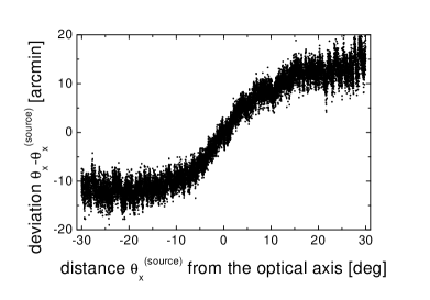
Figure 3: Deviation of the reconstructed event position $\theta_{x}$ from the nominal position $\theta_{x}^{\scriptsize{(source)}}$ as a function of the distance $\theta_{x}^{\scriptsize{(source)}}$ from the center of the field of view following from a correlation of Monte Carlo generated images with the unmodified mask pattern.

Furthermore, one observes a widening of the scatter of $\theta_{x}-\theta_{x}^{\scriptsize{(source)}}$ with increasing distance from the optical axis. This is due to the fact that the aberration, being proportional to the function $a_{\|}(\theta_{x},\theta_{y})$ to first order, is concave for $\theta_{x}>0$ and convex for $\theta_{x}<0$. The magnitude of this curvature increases with increasing distance from the origin.

3.1.3 Performance of the Algorithm

In order to disentangle the contributions from statistical scatter in the reconstruction from residual systematics, the dataset has been split into $N=20$ intervals in $\theta_{x}^{\scriptsize(source)}$. For each interval $i$ the mean value $\delta_{i}$ of $\theta_{x}^{\prime}-\theta_{x}^{\scriptsize(source)}$ as well as the standard deviation $\sigma_{i}$ has been derived. Because the intervals are chosen such that they cover an angular range of just $3^{\circ}$, the scatter $\sigma_{i}$ can be assumed to be dominated by statistics. An increase in photon number $n_{\gamma}$ per image would have reduced the statistical scatter, according to $\sigma_{i}\sim 1/\sqrt{n_{\gamma}}$.
From the values $\delta_{i}$ we derive the quantity $\delta=1/N\cdot\sqrt{\sum_{i}{\delta_{i}^{2}}}$, which is the mean quadratic deviation from zero. Further on, from $\sigma_{i}$ we determine the average statistical scatter $\sigma=1/N\cdot\sum_{i}\sigma_{i}$. From those two quantities, we define the spot size $\omega=\sqrt{\sigma^{2}+\delta^{2}}$.
Figure 4 illustrates the performance of the applied corrections: The mean quadratic deviation $\delta_{i}$ as well as the statistical error $\sigma_{i}$ is plotted against the angle of incidence $\theta_{x}^{\scriptsize(source)}$. As the flatness indicates, $\delta_{i}$ is consistent with zero, i.e. the imaging aberrations have been properly corrected. Moreover, $\sigma_{i}$ has become independent from the angle of incidence $\theta_{x}^{\scriptsize(source)}$, which indicates that the second order influence of $\theta_{y}^{\scriptsize(source)}$ on the reconstruction has been properly accounted for. Residual deviations are caused by detector nonlinearities, especially in the charge division method by which the position of an absorbed photon is determined.

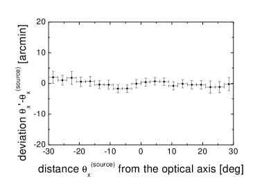
Figure 4: Deviation of the corrected event position $\theta_{x}^{\prime}$ from the nominal source position $\theta_{x}^{\scriptsize{(source)}}$ as a function of angle of incidence $\theta_{x}^{\scriptsize{(source)}}$ for the Monte Carlo generated dataset.

The mean statistical scatter has been determined to $\sigma=1.53^{\prime}\pm 0.29^{\prime}$ and the mean systematic deviation from zero to $\delta=1.00^{\prime}\pm 1.72^{\prime}$. The algorithm thus fulfills the design requirements. Figure 5 shows the result of combining the reconstructions in $x$- and $y$-direction. The scatter plot is circularly symmetric and the width of the spot corresponds to $\omega=1.83^{\prime}\pm 0.97^{\prime}$.

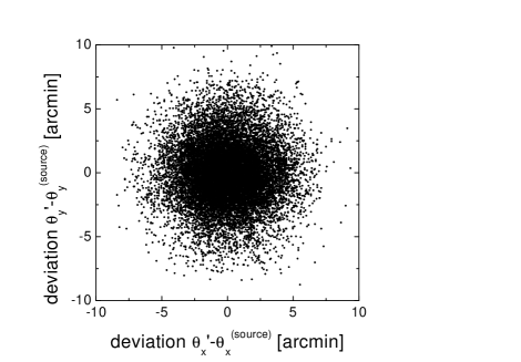
Figure 5: Scatter plot of all localisations $(\theta_{x}^{\prime}-\theta_{x}^{\scriptsize{(source)}},\theta_{y}^{\prime}-\theta_{y}^{\scriptsize{(source)}})$ for the Monte Carlo set of images.

In the above analysis, the value for the average attenuation length $a$ has been optimised is such a way that $\delta$ assumed a minimal value. The smallest deviations resulted in the choice $a=3.7\mbox{ mm}$, which is in agreement with the theoretical value $a=4.0\mbox{ mm}$. The theoretical value was derived by determining the flux weighted average of tabulated values for the photon attenuation length in xenon, where the photon spectrum has been altered by the spectral photon absorption probability.

3.2 Astrometric Observation of Scorpius X-1

3.2.1 Scorpius X-1 Data

Data from the X-ray source Scorpius X-1 has been taken for calibration purposes. Due to HETE-2’s antisolar pointing, any source will drift through the field of view at ecliptic rate, i.e. $\sim 1^{\circ}/\mbox{day}$. The orientation of the satellite was such that the WXM coordinate system was rotated $\sim 10^{\circ}$ relative to the celestial $(\alpha,\delta)$ frame. Scorpius X-1 was viewed at angles of incidence ranging from $\theta_{x}=-5^{\circ}$ to $\theta_{x}=+25^{\circ}$ and at $\theta_{y}=+5^{\circ}$ fixed. The spacecraft attitude was known to an accuracy surpassing $1^{\prime}$.

As pointed out in [12], the spectrum of Scorpius X-1, being a low-mass X-ray binary, can be described by a multicolour blackbody spectrum. Due to the integration time of $\Delta t=2\mbox{ sec}$, short term spectral changes like quasi-periodic oscillations average out. Long term variabilities either happen on significantly longer time scales compared to the data taking, or they affect energies outside HETE-2’s sensitivity interval. Determining the average attenuation length by a photon flux weighted integral with tabulated values for the attenuation length yielded $a=2.5\mbox{ mm}$. Thus, the spectrum of Scorpius X-1 is much softer compared to the previous case. The background subtracted images oconsisted roughly of $n_{\gamma}=3000$ photons.

3.2.2 Performance of the Algorithm

The analysis 3.1.3 is repeated for the Scorpius X-1 dataset. For each pointing $\delta_{i}$ and $\sigma_{i}$ have been derived. Figure 6 illustrates the accuracy of the source localisation algorithm. Again, the values $\delta_{i}$ with their errors $\sigma_{i}$ are shown as a function of angle of incidence $\theta_{x}^{\scriptsize(source)}$.

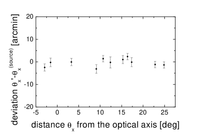
Figure 6: Deviation of the corrected event position $\theta_{x}^{\prime}$ from the nominal source position $\theta_{x}^{\scriptsize{(source)}}$ as a function of angle of incidence $\theta_{x}^{\scriptsize{(source)}}$ in the WXM-coordinate frame for the observation of Scorpius X-1.

The average quadratic deviation from zero has been determined to $\delta=1.59^{\prime}\pm 1.65^{\prime}$ which is slightly larger than in the previous case, but reflects inaccuracies in the satellite pointing. Furthermore, this value is probably underestimated because of the incomplete sampling of the field of view. The statistical error is marginally smaller due to larger photon numbers and has been derived to be $\sigma=1.31^{\prime}\pm 0.51^{\prime}$.

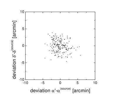
Figure 7: Scatter plot of all localisations $(\alpha^{\prime}-\alpha^{\scriptsize{(source)}},\delta^{\prime}-\delta^{\scriptsize{(source)}})$ in celestial coordinates. Scorpius X-1 is located at the origin.

Figure 7 shows the combined localisation in $x$- and $y$-direction, converted into the celestial coordinate frame. The radius of the spot is $\omega=2.06^{\prime}\pm 1.31^{\prime}$. The average attenuation length $a$ has been varied to yield the minimum value for $\delta$. In the case of Scorpius X-1, we find the optimum value to be $a=2.2\mbox{ mm}$, which corresponds well to the theoretically expected value $a=2.5\mbox{ mm}$.

4 Point Spread Function

4.1 Autocorrelation Function

In order to assess the extend to which angular resolving power is affected by the source localisation algorithm, the point spread function of the imaging system has been derived. For a coded mask camera like WXM, the point spread function is equal to the autocorrelation $s(x)$ of the mask pattern $m^{\prime\prime}(x)$, i.e. $s(x)=[m^{\prime\prime}\otimes m^{\prime\prime}](x)$. To be exact, $s(x)$ describes the isotropised point spread function. Anisotropies provoke asymmetries in the central correlation peak of the function $[m^{\prime\prime}\otimes m](x)$. Again, the determination of $s(x)$ is carried out in Fourier-space. Diagram 9 illustrates the derivation of $s(x)=\mathcal{F}^{-1}\left[|M^{\prime\prime}(k)|^{2}\right]$:

$$\lx@ams@matrix@{name=CD,datameaning=commutative-diagram}m(x)@>{\odot p(x)}>{}>m^{\prime}(x)@>{\odot r(x)}>{}>m^{\prime\prime}(x)@>{\otimes m^{\prime\prime}(x)}>{}>s(x)\\ @V{\mathcal{F}}V{}V@A{}A{\mathcal{F}^{-1}}A\\ M(k)@>{}>{\cdot P(k)}>M^{\prime}(k)@>{}>{\cdot R(k)}>M^{\prime\prime}(k)@>{}>{|\quad|^{2}}>S(k)\mbox{.}$$ (9)

4.2 Variations in Angular Resolving Power

The width $w_{x}$ of the autocorrelation function $s(x)$ has been determined by fitting a Gaussian to the central peak. The average width $w$ of the point spread function has been defined as the geometric mean of its extend in $x$- and $y$-direction ($w^{2}=w_{x}\cdot w_{y}$), because the quantity of interest is the size of the spot a source is imaged onto. The value of $s(x)$ at the origin corresponds to the correlation strength $v_{x}$. Accordingly, the average correlation strength $v$ has been defined to be equal to the arithmetic mean of $v_{x}$ and $v_{y}$ because of its analogy to brightness.

The angles of incidence have been restricted to $\left|\theta^{\scriptsize{(source)}}\right|=\sqrt{\theta_{x}^{2}+\theta_{y}^{2}}<20^{\circ}$, in order to ensure that the mask pattern is fully imaged onto the detector. The source positions were arranged on a square lattice with mesh size of $0.5^{\circ}$. The average attenuation length $a$ has been set to $3.7$ mm, corresponding to a power law spectrum with spectral index $\Gamma=1.1$.

The left plot in Figure 8 illustrates, that the width $w$ of the autocorrelation function increases and how the correlation strength decreases correspondingly at larger distances from the optical axis. At increasingly larger distance from the optical axis, the functions $p(x)$ and $p(y)$ disperse the correlation peak. Because the area underneath the peak has to be conserved, the correlation strength $v$ drops accordingly. Thus, the angular resolution power has decreased thus by $20\%$ for a burst at $\left|\theta^{\scriptsize(source)}\right|=20^{\circ}$ compared to a burst on the optical axis.

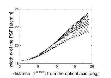
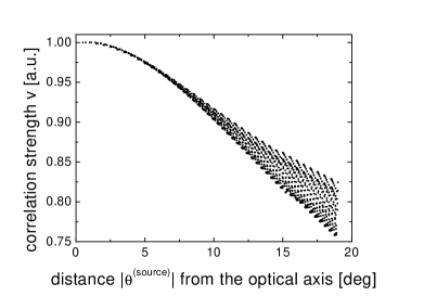
Figure 8: Average width $w$ in terms of FWHM (left) and correlation strength $v$ in arbitrary units (right) of the point spread function as a function of distance $\left|\theta^{\scriptsize(source)}\right|$ from the optical axis.

The scatter in Figure 8 is explained by the fact, that at fixed distance from the optical axis one obtains larger values of $w$ for a point situated on a diagonal than for a location on one of the axes, because in the latter case only one term is affected by the convolution with the functions $p(x)$ and $p(y)$ (formula 3). An analogous argument applies to the dependence of $v$ on the angles of incidence. This effect is of the order of $8\%$ at $\left|\theta^{\scriptsize(source)}\right|=20^{\circ}$.

5 Summary

This article describes an alternative correlation algorithm for $\gamma$-ray burst localisation with the WXM-device on board the HETE-2 satellite. The performance regarding source localisation accuracy has been validated using Monte Carlo simulated data and astrometric observations of the X-ray source Scorpius X-1.

• The algorithm corrects systematic deviations in the imaging process by convolving the mask pattern with suitable kernels. The convolution and the source reconstruction are both carried out in Fourier space, which is favourable with respect to time demand. Currently, the on board reconstruction algorithm relies on a library of Monte Carlo generated images.

• The Fourier algorithm is able to correct the systematic deviation caused by photons penetrating into the depth of the detector with high accuracy throughout the field of view (compare Table 1). The residual mean quadratic deviation is most likely due to nonlinearities in the detector response.

• The influence of the convolutions on angular resolving power have been investigated by determining the point spread function. One observes a widening of the correlation peak by $\sim 30\%$ together with a drop in correlation strength with increasing distance from the optical axis.

• The algorithm requires but a single, physically meaningful parameter: The average attenuation length $a$. Optimised values for $a$ correspond to theoretically expected values for a source with given spectral properties within $12\%$ (compare Table 2). Theoretical values follow from formula 10:

  $$a=\frac{\int\!\int\Phi(E)p(E,\vec{\theta})a(E)d^{2}\theta dE}{\int\!\int\Phi(E)p(E,\vec{\theta})d^{2}\theta dE}\mbox{,}$$ (10)

  where $\Phi(E)$ is the photon spectrum, $p(E,\vec{\theta})$ the probability of detecting a photon and $a(E)$ the attenuation length of a photon of energy $E$. Because of the spectral diversity of $\gamma$-ray bursts, it is necessary to compute $a$ for each event separately. In an on board application the weighted sum over a parameterisation of the function $a(E)$ would replace integral 10.

	Monte Carlo data		Scorpius X-1 data
	SD	FWHM	SD	FWHM
spot size $\omega$	$1.83^{\prime}\pm 0.97^{\prime}$	$4.31^{\prime}\pm 2.28^{\prime}$	$2.06^{\prime}\pm 1.31^{\prime}$	$4.85^{\prime}\pm 3.08^{\prime}$
systematic error $\delta$	$1.00^{\prime}\pm 1.72^{\prime}$	$2.35^{\prime}\pm 4.05^{\prime}$	$1.59^{\prime}\pm 1.65^{\prime}$	$3.74^{\prime}\pm 3.88^{\prime}$
statistical error $\sigma$	$1.53^{\prime}\pm 0.29^{\prime}$	$3.60^{\prime}\pm 0.68^{\prime}$	$1.31^{\prime}\pm 0.51^{\prime}$	$3.08^{\prime}\pm 1.20^{\prime}$

Table 1: Summary of the localisation performance of the algorithm, stated in standard deviation (SD) and full width half maximum (FWHM), for both the Monte Carlo simulation (left column) and the astrometric observation of Scorpius X-1 (right column).

	Monte Carlo data	Scorpius X-1 data
theoretical	$a=4.0\mbox{ mm}$	$a=2.5\mbox{ mm}$
experimental	$a=3.7\mbox{ mm}$	$a=2.2\mbox{ mm}$

Table 2: Comparison of theoretically expected with optimised values for the spectrally averaged attenuation length $a$ for different photon distributions. $a$ governs the correction for the imaging aberration due to photons penetrating into the depth of the detector.

References

- [1] W. S. Paciesas at al., preprint astro-ph/9903205
- [2] R. Jager et al., preprint astro-ph/9706065
- [3] L. Piro et al, Astron. Astrophys. 329, 906-910 (1998)
- [4] E. Costa et al., preprint astro-ph/9796965
- [5] N. Kawai et al., Astron. Astrophys. Suppl. Ser. 138, 563-564 (1999)
- [6] J.J.M. in’t Zand et al., Proceedings of ’Imaging in High-Energy Astronomy’, Capri (1994) yuji
- [7] Y. Shirasaki et al., Adv. Space Res. Vol. 25, No. 3/4, 893-896 (2000)
- [8] Y. Shirasaki et al., Proceedings of SPIE, Vol. 4012 (2000)
- [9] T.J. Ponman et al., NIM A262 (1987) 419-429
- [10] A. Hammersley et al., NIM A311 (1992) 585-594
- [11] T. E. Strohmayer et al., ApJ 500: 873-877 (1998)
- [12] K. Mitsuda et al., PASJ 36, 741-759 (1984)