$UBVRI$ Night sky brightness during sunspot maximum at ESO-Paranal

In this paper we present and discuss for the first time a large data set of $UBVRI$ night sky brightness measurements collected at ESO-Paranal from April 2000 to September 2001. A total of about 3900 images obtained on 174 different nights with FORS1 were analysed using an automatic algorithm specifically designed for this purpose. This led to the construction of an unprecedented database that allowed us to study in detail a number of effects such as differential zodiacal light contamination, airmass dependency, daily solar activity and moonlight contribution. Particular care was devoted to the investigation of short time scale variations and micro-auroral events. The typical dark time night sky brightness values found for Paranal are similar to those reported for other astronomical dark sites at a similar solar cycle phase. The zenith-corrected values averaged over the whole period are 22.3, 22.6, 21.6 20.9 and 19.7 mag arcsec^-2 in $U,B,V,R$ and $I$ respectively. In particular, there is no evidence of light pollution either in the broadband photometry or in the high-airmass spectra we have analysed. Finally, possible applications for the exposure time calculators are discussed.

1 Introduction

The night sky brightness, together with number of clear nights, seeing, transparency, photometric stability and humidity, are some of the most important parameters that qualify a site for front-line ground–based astronomy. While there is almost no way to control the other characteristics of an astronomical site, the sky brightness can be kept at its natural level by preventing light pollution in the observatory areas. This can be achieved by means of extensive monitoring programmes aimed at detecting any possible effects of human activity on the measured sky brightness.

For this purpose, we have started an automatic survey of the $UBVRI$ night sky brightness at Paranal with the aim of both getting for the first time values for this site and building a large database. The latter is a fundamental step for the long term trend which, given the possible growth of human activities around the observatory, will allow us to check the health of Paranal’s sky in the years to come.

The ESO-Paranal Observatory is located on the top of Cerro Paranal in the Atacama Desert in the northern part of Chile, one of the driest areas on Earth. Cerro Paranal (2635 m, 24^∘ 40^′ S, 70^∘ 25^′ W) is at about 108 km S of Antofagasta (225,000 inhabitants; azimuth 0^∘. 2), 280 km SW from Calama (121,000 inhabitants; azimuth 32^∘. 3), 152 km WSW from La Escondida (azimuth 32^∘. 9), 23 km NNW from a small mining plant (Yumbes, azimuth 157^∘. 7) and 12 km inland from the Pacific Coast. This ensures that the astronomical observations to be carried out there are not disturbed by adverse human activities like dust and light from cities and roads. Nevertheless, a systematic monitoring of the sky conditions is mandatory in order to preserve the high site quality and to take appropriate action, if the conditions are proven to deteriorate. Besides this, it will also set the stage for the study of natural sky brightness oscillations, both on short and long time scales, such as micro-auroral activity, seasonal and sunspot cycle effects.

The night sky radiation has been studied by several authors, starting with the pioneering work by Lord Rayleigh in the 1920s. For thorough reviews on this subject the reader is referred to the classical textbook by Roach & Gordon (roachgordon (1973)) and the recent extensive work by Leinert et al. (leinert98 (1998)), which explore a large number of aspects connected with the study of the night sky emission. In the following, we will give a short introduction to the subject, concentrating on the optical wavelengths only.

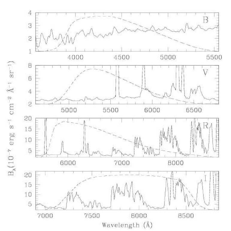
Figure 1: Night sky spectrum obtained at Paranal on February 25, 2001 02:38UT in the spectral region covered by $B$, $V$, $R$ and $I$ passbands (from top to bottom). The original FORS1 1800 seconds frame was taken at 1.42 airmasses with a long slit of 1^′′ and grism 150I, which provide a resolution of about 22 Å (FWHM). The dashed lines indicate the passband response curves. Flux calibration was achieved using the spectrophotometric standard star Feige 56 (Hamuy et al. 1992) observed during the same night. The absence of an order sorting filter probably causes some second order overlap at wavelengths redder than 6600 Å.

The night sky light as seen from ground is generated by several sources, some of which are of extra-terrestrial nature (e.g. unresolved stars/galaxies, diffuse galactic background, zodiacal light) and others are due to atmospheric phenomena (airglow and auroral activity in the upper Earth’s atmosphere). In addition to these natural components, human activity has added an extra source, namely the artificial light scattered by the troposphere, mostly in the form of Hg-Na emission lines in the blue-visible part of the optical spectrum (vapour lamps) and a weak continuum (incandescent lamps). While the extra-terrestrial components vary only with the position on the sky and are therefore predictable, the terrestrial ones are known to depend on a large number of parameters (season, geographical position, solar cycle and so on) which interact in a largely unpredictable way. In fact, airglow contributes with a significant fraction to the optical global night sky emission and hence its variations have a strong effect on the overall brightness.

To illustrate the various processes which contribute to the airglow at different wavelengths, in Figure 1 we have plotted a high signal-to-noise, flux calibrated night sky spectrum obtained at Paranal on a moonless night (2001, Feb 25) at a zenith distance of 45^∘ , about two hours after the end of evening astronomical twilight. In the $B$ band the spectrum is rather featureless and it is characterised by the so called airglow pseudo-continuum, which arises in layers at a height of about 90-100 km (mesopause). This actually extends from 4000Å to 7000Å and its intensity is of the order of 3$\times$10^-7 erg s^-1 cm^-2 Å^-1 sr^-1 at 4500Å. All visible emission features, which become particularly marked below 4000Å and largely dominate the $U$ passband (not included in the plots), are due to Herzberg and Chamberlain O₂ bands (Broadfoot & Kendall 1968). In light polluted sites, this spectral region is characterised by the presence of Hg I (3650, 3663, 4047, 4078, 4358 and 5461Å) and NaI (4978, 4983, 5149 and 5153Å) lines (see for example Osterbrock & Martel, 1992) which are, if any, very weak in the spectrum of Figure 1 (see Sec. 9 for a discussion on light pollution at Paranal). Some of these lines are clearly visible in spectra taken, for example, at La Palma (Benn & Ellison 1998, Figure 1) and Calar Alto (Leinert et al. 1995, Figs. 7 and 8).

The $V$ passband is chiefly dominated by [OI]5577Å and to a lesser extent by NaI D and [OI]6300,6364Å doublet. In the spectrum of Figure 1 the relative contribution to the total flux of these three lines is 0.17, 0.03 and 0.02, respectively. Besides the aforementioned pseudo-continuum, several OH Meinel vibration-rotation bands are also present in this spectral window (Meinel 1950); in particular, OH(8-2) is clearly visible on the red wing of NaI D lines and OH(5-0), OH(9-3) on the blue wing of [OI]6300Å. All these features are known to be strongly variable and show independent behaviour (see for example the discussion in Benn & Ellison 1998), probably due to the fact that they are generated in different atmospheric layers (Leinert et al. 1998 and references therein). In fact, [OI]5577Å, which is generally the brightest emission line in the optical sky spectrum, arises in layers at an altitude of 90 km, while [OI]6300,6364Å is produced at 250-300 km. The OH bands are emitted by a layer at about 85 km, while the Na ID is generated at about 92 km, in the so called Sodium-layer which is used by laser guide star adaptive optic systems. In particular, [OI]6300,6364Å shows a marked and complex dependency on geomagnetic latitude which turns into different typical line intensities at different observatories (Roach & Gordon roachgordon (1973)). Moreover, this doublet undergoes abrupt intensity changes (Barbier 1957); an example of such an event is reported and discussed in Sec. 9.

In the $R$ passband, besides the contribution of NaI D and [OI]6300,6364Å, which account for 0.03 and 0.10 of the total flux in the spectrum of Figure 1, strong OH Meinel bands like OH(7-2), OH(8-3), OH(4-0), OH(9-4) and OH(5-1) begin to appear, while the pseudo-continuum remains constant at about 3$\times$10^-7 erg s^-1 cm^-2 Å^-1 sr^-1. Finally, the $I$ passband is dominated by the Meinel bands OH(8-3), OH(4-0), OH(9-4), OH(5-1) and OH(6-2); the broad feature visible at 8600-8700Å, and marginally contributing to the $I$ flux, is the blend of the R and P branches of O₂(0-1) (Broadfoot & Kendall 1968).

Several sky brightness surveys have been performed at a number of observatories in the world, most of the time in $B$ and $V$ passbands using small telescopes coupled to photo-multipliers. A comprehensive list of published data is given by Benn & Ellison (benn (1998)). All authors agree on the fact that the dark time sky brightness shows strong variations within the same night on the time scales of tens of minutes to hours. This variation is commonly attributed to airglow fluctuations. Moreover, as first pointed out by Rayleigh (rayleigh (1928)), the intensity of the [OI]5577Å line depends on the solar activity. Similar results were found for other emission lines (NaI D and OH) by Rosenberg & Zimmerman (rosenberg (1967)). Walker (1988b ) found that $B$ and $V$ sky brightness is well correlated with the 10.7 cm solar radio flux and reported a range of $\sim$ 0.5 mag in $B$ and $V$ during a full sunspot cycle. Similar values were found by Krisciunas (krisc90 (1990)), Leinert et al. (leinert95 (1995)) and Mattila et al. (attila (1996)), so that the effect of solar activity is commonly accepted (Leinert et al. 1998). For this reason, when comparing sky brightness measurements, one should also keep in mind the time when they were obtained with respect to the solar cycle, since the difference can be substantial. A matter of long debate has been the so-called Walker effect, named after Walker (1988b ), who reported a steady exponential decrease of $\sim$0.4 mag in the night sky brightness during the first six hours following the end of twilight. This finding has been questioned by several authors. We address this issue in detail later (Sec. 6 and Appendix D).

Here we present for the first time $UBVRI$ sky brightness measurements for Paranal, obtained on 174 nights from 2000 April 20 to 2001 September 23 which, to our knowledge, makes it the largest homogeneous data set available. Being produced by an automatic procedure, this data base is continuously growing and it will provide an unprecedented chance to investigate both the long term evolution of the night sky quality and to study in detail the short time scale fluctuations which are still under debate.

The paper is organized as follows. After giving some information on the basic data reduction procedure in Sec. 2, in Sec. 3 we discuss the photometric calibration and error estimates, while the general properties of our night sky brightness survey are described in Sec. 4. The results obtained during dark time are then presented in Sec. 5 and the short time-scale variations are analysed in Sec. 6. In Sec. 7 we compare our data obtained in bright time with the model by Krisciunas & Schaefer (krischae (1991)) for the effects of moonlight, while the dependency on solar activity is investigated in Sec. 8. In Sec. 9 we discuss the results and summarize our conclusions. Finally, detailed discussions about some of the topics are given in Appendices A–D.

2 Observations and basic data reduction

The data set discussed in this work has been obtained with the FOcal Reducer/low dispersion Spectrograph (hereafter FORS1), mounted at the Cassegrain focus of ESO–Antu/Melipal 8.2m telescopes (Szeifert 2002). The instrument is equipped with a 2048$\times$2048 pixels (px) TK2048EB4-1 backside thinned CCD and has two remotely exchangeable collimators, which give a projected scale of 0″. 2 and 0″. 1 per pixel (24$\mu$m $\times$ 24$\mu$m). According to the used collimator, the sky area covered by the detector is 6′. 8$\times$6′. 8 and 3′. 4$\times$3′. 4, respectively. Most of the observations discussed in this paper were performed with the lower resolution collimator, since the higher resolution is used only to exploit excellent seeing conditions (FWHM$\leq$0″. 4).

In the current operational scheme, FORS1 is offered roughly in equal fractions between visitor mode (VM) and service mode (SM). While VM data are immediately released to the visiting astronomers, the SM data are processed by the FORS-Pipeline and then undergo a series of quality control (QC) checks before being delivered to the users. In particular, the imaging frames are bias and flat-field corrected and the resulting products are analysed in order to assess the accuracy of the flat-fielding, the image quality and so on. The sky background measurement was experimentally introduced in the QC procedures starting with April 2000. Since then, each single imaging frame obtained during SM runs is used to measure the sky brightness. During the first eighteen months of sky brightness monitoring, more than 4500 frames taken with broad and narrow band filters have been analysed.

As already mentioned, all imaging frames are automatically bias and flat field corrected by the FORS pipeline. This is a fundamental step, since in the case of imaging, the FORS1 detector is readout using four amplifiers which have different gains. The bias and flat field correction remove the four-port structure to within $\sim$1 electron. This has to be compared with the RMS read-out noise (RON), which is 5.5 and 6.3 electrons in the high gain and low gain modes respectively. Moreover, due to the large collecting area of the telescope, FORS1 imaging frames become sky background dominated already after less than two minutes. The only significant exception is the $U$ passband, where background domination occurs after more than 10 minutes (see also Table 1). The dark current of FORS1 detector is $\sim$2.2 $\times$ 10^-3 e^- s^-1 px^-1 (Szeifert szeifert (2000)) and hence its contribution to the background can be safely neglected.

Table 1: Typical background count rates expected in FORS1 (SR) images during dark time and at zenith. The last column reports the time required to have a background photon shot noise three times larger than the maximum RON (6.3 $e^{-}$), which corresponds to a 5% contribution of RON to the global noise.

Passband	Count Rate	$t_{3}$
	(e- px-1 s-1)	(s)
U	0.5	714
B	3.8	94
V	15.8	23
R	26.7	13
I	32.1	11

Since the flat fielding is performed using twilight sky flats, some large scale gradients are randomly introduced by the flat fielding process; maximum peak-to-peak residual deviations are of the order of 6$\%$. Finally, small scale features are very well removed, the only exceptions being some non-linear pixels spread across the detector.

The next step in the process is the estimate of the sky background. Since the science frames produced by FORS1 are, of course, not necessarily taken in empty fields, the background measurement requires a careful treatment. For this purpose we have designed a specific algorithm, which is presented and discussed in Patat (patat (2002)). The reader is referred to that paper for a detailed description of the problem and the technique we have adopted to solve it.

3 Photometric calibration and global errors

Once the sky background $I_{sky}$ has been estimated, the flux per square arcsecond and per unit time is given by $f_{sky}=I_{sky}/(t_{exp}\;p^{2})$, where $p$ is the detector’s scale (arcsec pix^-1) and $t_{exp}$ is the exposure time (in seconds). The instrumental sky surface brightness is then defined as

$$m_{sky}=-1.086\;ln(I_{sky})+2.5\;log(p^{2}\;t_{exp})$$ (1)

with $m_{sky}$ expressed in mag arcsec^-2. Neglecting the errors on $p$ and $t_{exp}$, one can compute the error on the sky surface brightness as $\delta_{b_{sky}}\simeq\delta_{I_{sky}}/I_{sky}$. This means, for instance, that an error of 1% on $I_{sky}$ produces an uncertainty of 0.01 mag arcsec^-2 on the final instrumental surface brightness estimate. While in previous photoelectric sky brightness surveys the uncertainty on the diaphragm size contributes to the global error in a relevant way (see for example Walker 1988b), in our case the pixel scale is known with an accuracy of better than 0.03 % (Szeifert 2002) and the corresponding photometric error can therefore be safely neglected.

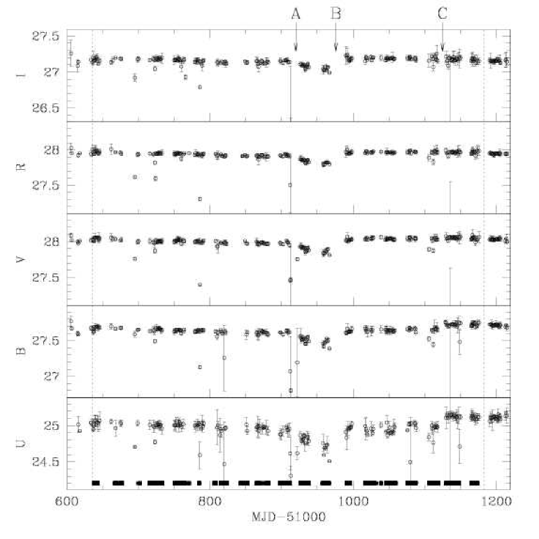
Figure 2: UBVRI photometric zeropoints for FORS1 during the time range covered by sky brightness measurements presented in this work (vertical dotted lines). The thick segments plotted on the lower diagram indicate the presence of sky brightness data, while the arrows in the upper part of the figure correspond to some relevant events. A: water condensation on main mirror of UT1-Antu. B: UT1-Antu main mirror re-aluminisation after the water condensation event. C: FORS1 moved from UT1-Antu to UT3-Melipal. Plotted zeropoints have been corrected for extinction and colour terms using average values (see Appendix A).

The next step one needs to perform to get the final sky surface brightness is to convert the instrumental magnitudes to the standard $UBVRI$ photometric system. Following the prescriptions by Pilachowski et al. (pila (1989)), the sky brightness is calibrated without correcting the measured flux by atmospheric extinction, since the effect is actually taking place mostly in the atmosphere itself. This is of course not true for the contribution coming from faint stars, galaxies and the zodiacal light, which however account for a minor fraction of the whole effect, airglow being the prominent source of night sky emission in dark astronomical sites. The reader is referred to Krisciunas (krisc90 (1990)) for a more detailed discussion of this point; here we add only that this practically corresponds to set to zero the airmass of the observed sky area in the calibration equation. Therefore, if $M_{sky}$, $m_{sky}$ are the calibrated and instrumental sky magnitudes, $M_{*}$, $m_{*}$ are the corresponding values for a photometric standard star observed at airmass $z_{*}$, and $\kappa$ is the extinction coefficient, we have that $M_{sky}=(m_{sky}-m_{*})+\kappa\;z_{*}+M_{*}+\gamma\;(C_{sky}-C_{*})$. This relation can be rewritten in a more general way as $M_{sky}=m_{0}+m_{sky}+\gamma\;C_{sky}$, where $m_{0}$ is the photometric zeropoint in a given passband and $\gamma$ is the colour term in that passband for the color $C_{sky}$. For example, in the case of B filter, this relation can be written as $B_{sky}=B_{0}+b_{sky}+\gamma^{B}_{B-V}\;(B-V)_{sky}$.

In the case of FORS1, observations of photometric standard fields (Landolt 1992) are regularly obtained as part of the calibration plan; typically one to three fields are observed during each service mode night. The photometric zeropoints were derived from these observations by means of a semi-automatic procedure, assuming constant extinction coefficients and colour terms. For a more detailed discussion on these parameters, the reader is referred to Appendix A, where we show that this is a reasonable assumption. Figure 2 shows that, with the exception of a few cases, Paranal is photometrically stable, being the RMS zeropoint fluctuation $\sigma_{m_{0}}$=0.03 mag in $U$ and $\sigma_{m_{0}}$=0.02 mag in all other passbands. Three clear jumps are visible in Figure 2, all basically due to physical changes in the main mirror of the telescope. Besides these sudden variations, we have detected a slow decrease in the efficiency which is clearly visible in the first 10 months and is most probably due to aluminium oxidation and dust deposition. The efficiency loss appears to be linear in time, with a rate steadily decreasing from blue to red passbands, being 0.13 mag yr^-1 in $U$ and 0.05 mag yr^-1 in $I$. To allow for a proper compensation of these effects, we have divided the whole time range in four different periods, in which we have used a linear least squares fit to the zero points obtained in each band during photometric nights only. This gives a handy description of the overall system efficiency which is easy to implement in an automatic calibration procedure.

Table 2: Typical night sky broad band colours measured at various observatories.

Site	Year	$U-B$	$B-V$	$V-R$	$V-I$	Reference
Cerro Tololo	1987-8	$-$0.7	+0.9	+0.9	+1.9	Walker (1987, 1988a)
La Silla	1978	-	+1.1	+0.9	+2.3	Mattila et al. (1996)
Calar Alto	1990	$-$0.5	+1.1	+0.9	+2.8	Leinert et al. (1995)
La Palma	1994-6	$-$0.7	+0.8	+0.9	+1.9	Benn & Ellison (1998)
Paranal	2000-1	$-$0.4	+1.0	+0.8	+1.9	this work

To derive the colour correction included in the calibration equation one needs to know the sky colours $C_{sky}$. In principle $C_{sky}$ can be computed from the instrumental magnitudes, provided that the data which correspond to the two passbands used for the given colour are taken closely in time. In fact, the sky brightness is known to have quite a strong time evolution even in moonless nights and far from twilight (Walker 1988b, Pilachowski et al. 1989, Krisciunas 1990, Leinert et al. 1998) and using magnitudes obtained in different conditions would lead to wrong colours. On the other hand, very often FORS1 images are taken in rather long sequences, which make use of the same filter; for this very reason it is quite rare to have close-in-time multi-band observations. Due to this fact and to allow for a general and uniform approach, we have decided to use constant sky colours for the colour correction. In fact, the colour terms are small, and even large errors on the colours produce small variations in the corresponding colour correction.

For this purpose we have used color-uncorrected sky brightness values obtained in dark time, at airmass $z\leq 1.3$ and at a time distance from the twilights $\Delta t_{twi}\geq 2.5$ hours and estimated the typical value as the average. The corresponding colours are shown in Table 2, where they are compared with those obtained at other observatories. As one can see, $B-V$ and $V-R$ show a small scatter between different observatories, while $U-B$ and $V-I$ are rather dispersed. In particular, $V-I$ spans almost a magnitude, the value reported for Calar Alto being the reddest. This is due to the fact that the Calar Alto sky in $I$ appears to be definitely brighter than in all other listed sites.

Now, given the color terms reported in Table 7, the color corrections $\gamma\times C_{sky}$ turn out to be $-$0.02$\pm$0.02, $-$0.09$\pm$0.02, +0.04$\pm 0.01$, +0.02$\pm$0.01 and $-$0.08$\pm$0.02 in $U$, $B$, $V$, $R$ and $I$ respectively. The uncertainties were estimated from the dispersion on the computed average colours, which is $\sigma_{C}\simeq$0.3 for all passbands. We emphasize that this rather large value is not due to measurement errors, but rather to the strong intrinsic variations shown by the sky brightness, which we will discuss in detail later on. We also warn the reader that the colour corrections computed assuming dark sky colours are not necessarily correct under other conditions, when the night sky emission is strongly influenced by other sources, like Sun and moon. At any rate, colour variations of 1 mag would produce a change in the calibrated magnitude of $\sim$0.1 mag in the worst case.

Due to the increased depth of the emitting layers, the sky becomes inherently brighter for growing zenith distances (see for example Garstang 1989, Leinert et al. 1998). In order to compare and/or combine together sky brightness estimates obtained at different airmasses, one needs to take into account this effect. The law we have adopted for the airmass compensation and its ability to reproduce the observed data are discussed in Appendix C (see Eq. 10). After including this correction in the calibration equation and neglecting the error on $X$, we have computed the global RMS error on the estimated sky brightness in the generic passband as follows:

$$\sigma_{M_{sky}}\simeq\sqrt{\delta^{2}_{m_{sky}}+\sigma^{2}_{m_{0}}+\gamma^{2}\;\sigma^{2}_{C}+C^{2}\;\sigma^{2}_{\gamma}+(X-1)^{2}\;\sigma^{2}_{\kappa}}$$ (2)

where $\sigma_{m_{0}}$, $\sigma_{C}$, $\sigma_{\gamma}$ and $\sigma_{K}$ are the uncertainties on the zero point, sky colour, colour term and extinction coefficient respectively. Using the proper numbers one can see that the typical expected global error is 0.03$\div$0.04 mag, with the measures in $V$ and $R$ slightly more accurate than in $U$, $B$ and $I$.

4 ESO-Paranal night sky brightness survey

The results we will discuss have been obtained between April 1 2000 and September 30 2001, corresponding to ESO Observing Periods 65, 66 and 67, and include data obtained on 174 different nights. During these eighteen months, 4439 images taken in the $UBVRI$ passbands and processed by the FORS pipeline were analysed and 3883 of them ($\sim$88%) were judged to be suitable for sky brightness measurements, according to the criteria we have discussed in Patat (patat (2002)). The numbers for the different passbands are shown in Table 3, where we have reported the total number $N_{t}$ of examined frames, the number $N_{s}$ of frames which passed the tests and the percentage of success $f_{s}$. As expected, this is particularly poor for the $U$ filter, where the sky background level is usually very low. In fact, we have shown that practically all frames with a sky background level lower than 400 electrons are rejected (Patat patat (2002), Sec. 5). Since to reach this level in the $U$ passband one needs to expose for more than 800 seconds (see Table 1), this explains the large fraction of unacceptable frames. We also note that the number of input frames in the various filters reflects the effective user’s requests. As one can see from Table 3, the percentage of filter usage $f_{t}$ steadily grows going from blue to red filters, with $R$ and $I$ used in almost 70% of the cases, while the $U$ filter is extremely rarely used.

Table 3: Number of sky brightness measurements obtained with FORS1 in $U,B,V,R,I$ passbands from April 1, 2000 to September 30, 2001.

Filter	$f_{t}$ (%)	$N_{t}$	$N_{s}$	$f_{s}$ (%)
U	1.8	204	68	33.3
B	11.3	479	434	90.6
V	17.3	845	673	79.6
R	27.1	1128	1055	93.5
I	42.5	1783	1653	92.7
		4439	3883	87.5

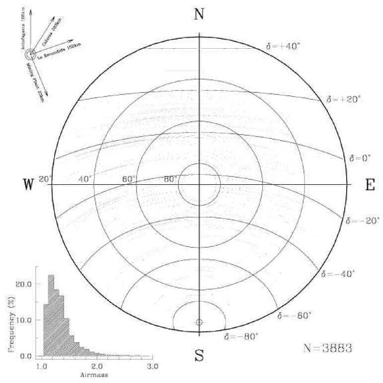
Figure 3: Distribution of telescope pointings in Alt-Az coordinates. The lower left insert shows the airmass distribution.

To allow for a thorough analysis of the data, the sky brightness measurements have been logged together with a large set of parameters, some of which are related to the target’s position and others to the ambient conditions. The first set has been computed using routines adapted from those coded by J. Thorstensen and it includes average airmass, azimuth, galactic longitude and latitude, ecliptic latitude and helio-ecliptic longitude, target-moon angular distance, moon elevation, fractional lunar illumination (FLI), target-Sun angular distance, Sun elevation and time distance between observation and closest twilight. Additionally we have implemented two routines to compute the expected moon brightness and zodiacal light contribution at target’s position. For the first task we have adopted the model by Krisciunas & Schaefer (krischae (1991)) and its generalisation to $UBVRI$ passbands (Schaefer 1998), while for the zodiacal light we have applied a bi-linear interpolation to the data presented by Levasseur-Regourd & Dumont (levasseur (1980)). The original data is converted from $S_{10}(V)$ to $cgs$ units and the $UBRI$ brightness is computed from the $V$ values reported by Levasseur-Regourd & Dumont assuming a solar spectrum, which is a good approximation in the wavelength range 0.2$-$2$\mu$m (Leinert et al. 1998). For this purpose we have adopted the Sun colours reported by Livingston (livingston (2000)), which turn into the following $U$, $B$, $R$ and $I$ zodiacal light intensities normalised to the $V$ passband: 0.52, 0.94, 0.77 and 0.50. For a derivation of the conversion factor from $S_{10}(V)$ to $cgs$ units, see Appendix B.

The ambient conditions were retrieved from the VLT Astronomical Site Monitor (ASM, Sandrock et al. 2000). For our purposes we have included air temperature, relative humidity, air pressure, wind speed and wind direction, averaging the ASM entries across the exposure time. Finally, to allow for further quality selections, for each sky brightness entry we have logged the number of sub-windows which passed the $\Delta$-test (see Patat patat (2002)) and the final number $n_{g}$ of selected sub-windows effectively used for the background estimate.

Throughout this paper the sky brightness is expressed in mag arcsec^-2, following common astronomical practice. However, when one is to correct for other effects (like zodiacal light or scattered moon light), it is more practical to use a linear unit. For this purpose, when required, we have adopted the $cgs$ system, where the sky brightness is expressed in erg s^-1 cm^-2 Å^-1 sr^-1. In these units the typical sky brightness varies in the range 10${}^{-9}-10^{-6}$ (see also Appendix B). It is natural to introduce a surface brightness unit (sbu) defined as 1 sbu$\equiv$10^-9 erg s^-1 cm^-2 Å^-1 sr^-1. In the rest of the paper we will use this unit to express the sky brightness in a linear scale.

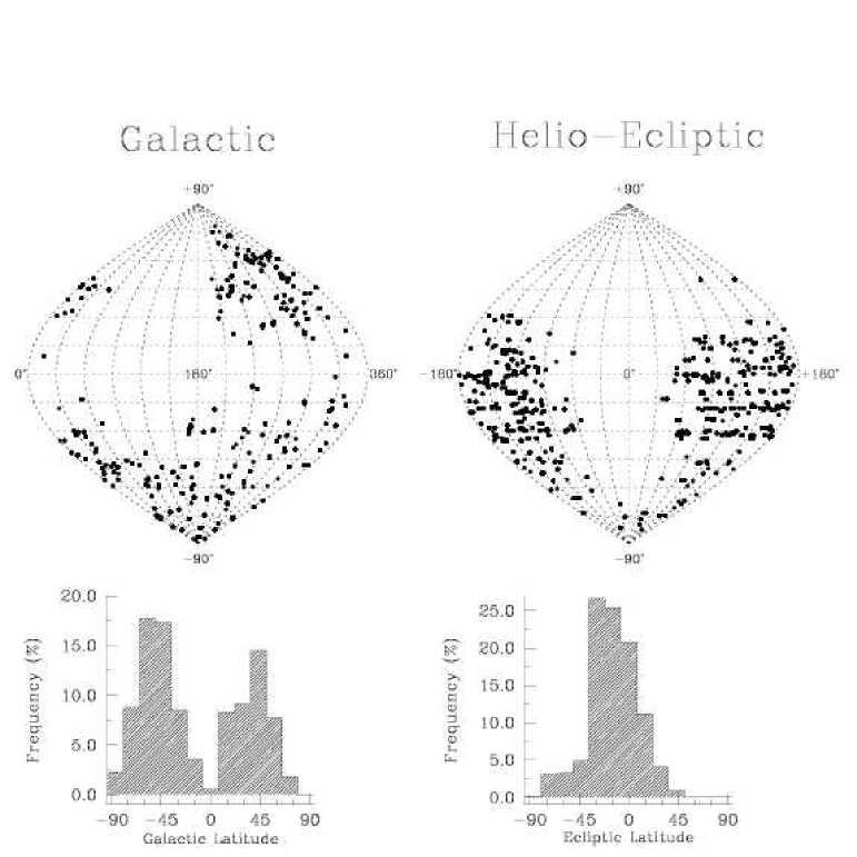
Figure 4: Distribution of telescope pointings in galactic (left panel) and helio-ecliptic (right panel) coordinates. The two histograms show the distribution of galactic and ecliptic latitudes.

Due to the large number of measurements, the data give a good coverage of many relevant parameters. This is fundamental, if one is to investigate possible dependencies. In the next sub-sections we describe the statistical properties of our data set with respect to these parameters, whereas their correlations are discussed in Secs. 5-8.

4.1 Coordinate distribution

The telescope pointings are well distributed in azimuth and elevation, as it is shown in Figure 3. In particular, they span a good range in airmass, with a few cases reaching zenith distances larger than 60^∘. Due to the Alt-Az mount of the VLT, the region close to zenith is not observable, while for safety reasons the telescope does not point at zenith distances larger than 70^∘. Apart from these two avoidance areas, the Alt-Az space is well sampled, at least down to zenith distances $Z$=50^∘. At higher airmasses the western side of the sky appears to be better sampled, due to the fact that the targets are sometimes followed well after the meridian, while the observations tend to start when they are on average at higher elevation.

Since sky brightness is expected to depend on the observed position with respect to the Galaxy and the Ecliptic (see Leinert et al. 1997 for an extensive review), it is interesting to see how our measurements are distributed in these two coordinate systems. Due to the kind of scientific programmes which are usually carried out with FORS1, we expect that most of the observations are performed far from the galactic plane. This is confirmed by the left panel of Figure 4, where we have plotted the galactic coordinates distribution of the 3883 pointing included in our data set. As one can see, the large majority of the points lie at $|b|>$10^∘, and therefore the region close to the galactic plane is not well enough sampled to allow for a good study of the sky brightness behaviour in that area.

The scenario is different if we consider the helio-ecliptic coordinate system (Figure 4, right panel). The observations are well distributed across the ecliptic plane for $|\lambda-\lambda_{\odot}|>$60^∘ and $\beta<$+30^∘, where the contribution of the zodiacal light to the global sky brightness can be significant. As a matter of fact, the large majority of the observations have been carried out in the range $-$30${}^{\circ}\leq\beta\leq+$30^∘, where the zodiacal light is rather important at all helio-ecliptic longitudes. This is clearly visible in the upper panel of Figure 5, where we have over imposed the telescope pointings on a contour plot of the zodiacal light $V$ brightness, obtained from the data published by Levasseur-Regourd & Dumont (levasseur (1980)).

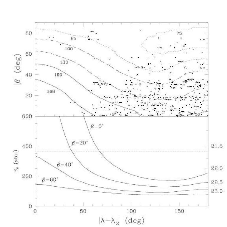
Figure 5: Upper panel: distribution of telescope pointings in helio-ecliptic coordinates. Over imposed is a contour plot of the zodiacal light $V$ brightness at the indicated levels expressed in sbu (1 sbu = 10^-9 erg s^-1 cm^-2 Å^-1 sr^-1). Original data are from Levasseur-Regourd & Dumont (levasseur (1980)). Lower panel: Zodiacal light $V$ brightness profiles at four different ecliptic latitudes expressed in sbu (left scale) and mag arcsec^-2 (right scale). The brightness increase seen at $|\lambda-\lambda_{\odot}|>$150^∘ is the so-called Gegenschein. The horizontal dotted line is placed at a typical $V$ global sky brightness during dark time (21.6 mag arcsec^-2).

We note that the wavelength dependency of the zodiacal light contribution is significant even within the optical range. In particular it reaches its maximum contribution in the $B$ passband, where the ratio between zodiacal light and typical dark time sky flux is always larger than 30%. On the opposite side we have the $I$ passband, where for $|\lambda-\lambda_{\odot}|\geq$80^∘ the contribution is always smaller than 30% (see also O’Connell 1987). Now, using the data from Levasseur-Regourd & Dumont (levasseur (1980)) and the typical dark time sky brightness measured on Paranal, we can estimate the sky brightness variations one expects on the basis of the pure effect of variable zodiacal light contribution. As we have already mentioned, the largest variation is expected in the $B$ band, where already at $|\lambda-\lambda_{\odot}|$=90^∘ the sky becomes inherently brighter by 0.4-0.5 mag as one goes from $|\beta|>$60^∘ to $|\beta|=$0^∘. This variation decreases to $\sim$0.15 mag in the $I$ passband.

Due to the fact that the bulk of our data has been obtained at $|\beta|\leq$30^∘, our dark time sky brightness estimates are expected to be affected by systematic zodiacal light effects, which have to be taken into account when comparing our results with those obtained at high ecliptic latitudes for other astronomical sites (see Sec. 5).

4.2 Moon Contribution

Another relevant aspect that one has to take into account when measuring the night sky brightness is the contribution produced by scattered moon light. Due to the scientific projects FORS1 was designed for, the large majority of observations are carried out in dark time, either when the fractional lunar illumination (FLI) is small or when the moon is below the horizon. Nevertheless, according to the user’s requirements, some observations are performed when moon’s contribution to the sky background is not negligible. To evaluate the amount of moon light contamination at a given position on the sky (which depends on several parameters, like target and moon elevation, angular distance, FLI and extinction coefficient in the given passband) we have used the model developed by Krisciunas and Schaefer (krischae (1991)), with the double aim of selecting those measurements which are not influenced by moonlight and to test the model itself. We have forced the lunar contribution to be zero when moon elevation is $h_{m}\leq-$18^∘ and we have neglected any twilight effects. On the one hand this has certainly the effect of overestimating the moon contribution when $-$18${}^{\circ}\leq h_{m}\leq$0^∘, but on the other hand it puts us on the safe side when selecting dark time data.

As expected, a large fraction of the observations were obtained practically with no moon: in more than 50% of the cases moon’s addition is from 10^-1 to 10^-3 the typical dark sky brightness. Nevertheless, there is a substantial tail of observations where the contamination is relevant (200$-$400 sbu) and a few extreme cases were the moon is the dominating source ($>$600 sbu). This offers us the possibility of exploring both regimes.

4.3 Solar activity

We conclude the description of the statistical properties of our data set by considering the solar activity during the relevant time interval. As it has been first pointed out by Lord Rayleigh (rayleigh (1928)), the airglow emission is correlated with the sunspot number. As we have seen in Sec. 1, this has been confirmed by a number of studies and is now a widely accepted effect (see Walker 1988b and references therein). As a matter of fact, all measurements presented in this work were taken very close to the maximum of sunspot cycle n. 23, and thus we do not expect to see any clear trend. This is shown in Figure 6, where we have plotted the monthly averaged Penticton-Ottawa solar flux at 2800 MHz (Covington 1969). We notice that the solar flux abruptly changed by a factor $\sim$2 between July and September 2001, leading to a second maximum which lasted roughly two months at the end of year 2001. This might have some effect on our data, which we will discuss later on.

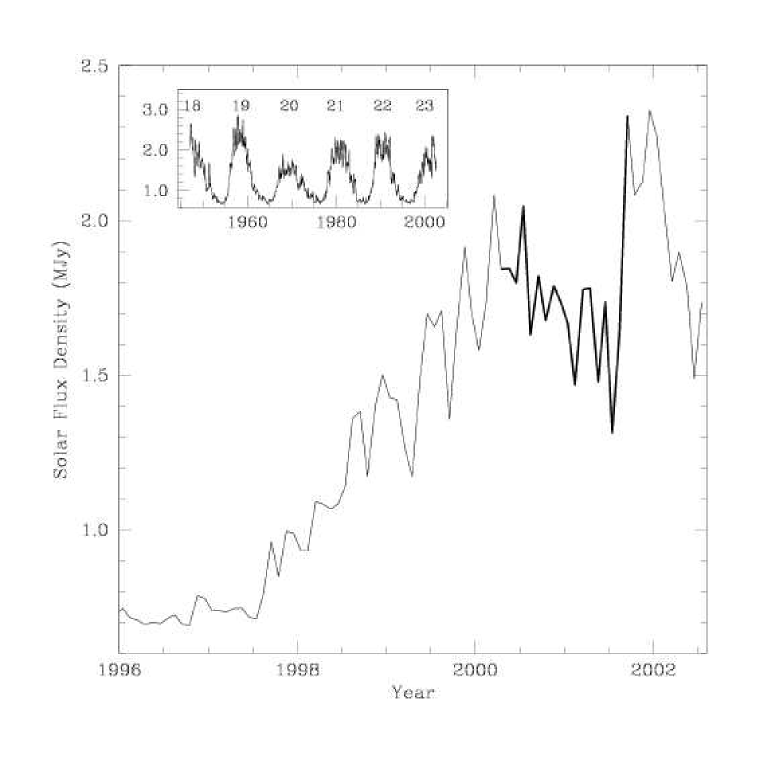
Figure 6: Penticton-Ottawa Solar flux at 2800 MHz (monthly average). The time range covered by the data presented in this paper is indicated by the thick line. The upper left insert traces the solar flux during the last six cycles.

5 Dark time sky brightness at Paranal

Due to the fact that our data set collects observations performed under a wide range of conditions, in order to estimate the zenith sky brightness during dark time it is necessary to apply some selection. For this purpose we have adopted the following criteria: photometric conditions, airmass $X\leq$1.4, galactic latitude $|b|>$10^∘, time distance from the closest twilight $\Delta t_{twi}>$1 hour and no moon (FLI=0 or $h_{M}\leq-$18^∘). Unfortunately, as we have mentioned in Sec. 4.1, very few observations have been carried out at $|\beta|>$45^∘ and hence we could not put a very stringent constraint on the ecliptic latitude, contrary to what is usually done (see for example Benn & Ellison 1998). To limit the contribution of the zodiacal light, we could only restrict the range of helio-ecliptic longitude ($|\lambda-\lambda_{\odot}|\geq$90^∘). The results one obtains from this selection are summarized in Table 4 and Figure 7, where we have plotted the estimates of the sky brightness at zenith as a function of time. Once one has accounted for the zodiacal light bias (see below), the values are consistent with those reported for other dark sites; in particular, they are very similar to those presented by Mattila et al. (attila (1996)) for La Silla, which were also obtained during a sunspot maximum (February 1978). As pointed out by several authors, the dark time values show quite a strong dispersion, which is typically of the order of 0.2 mag RMS. Peak to peak variations in the $V$ band are as large as 0.8 mag, while this excursion reaches 1.5 mag in the $I$ band.

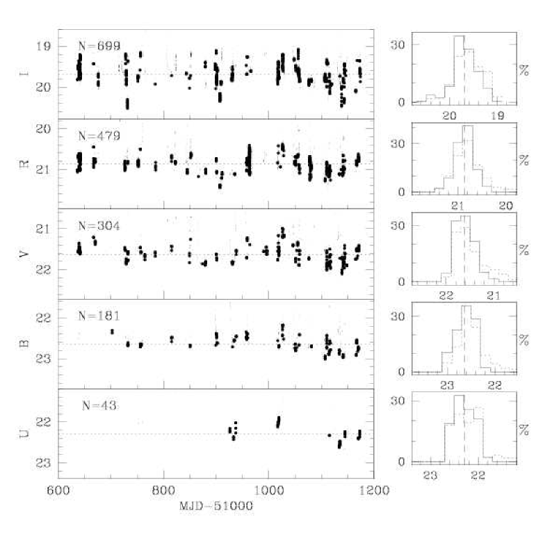
Figure 7: Zenith corrected sky brightness measured at Paranal during dark time (thick dots) from April 1st, 2000 to September 30th, 2001. The selection criteria are: $|b|>$10^∘, $|\lambda-\lambda_{\odot}|\geq$90^∘, $\Delta t_{twi}>$1 hour, FLI=0 or $h_{m}\leq-$18^∘. Thin dots indicate all observations (corrected to zenith). The horizontal dotted lines are positioned at the average values of the selected points. The histograms trace the distribution of selected measurements (solid line) and all measurements (dotted line), while the vertical dashed lines are placed at the average sky brightness during dark time.

Table 4: Zenith corrected average sky brightness during dark time at Paranal. Values are expressed in mag arcsec^-2. Columns 3 to 7 show the RMS deviation, minimum and maximum brightness, number of data points and expected average contribution from the zodiacal light, respectively.

Filter	Sky Br.	$\sigma$	Min	Max	N	$\Delta m_{ZL}$
U	22.28	0.22	21.89	22.61	39	0.18
B	22.64	0.18	22.19	23.02	180	0.28
V	21.61	0.20	20.99	22.10	296	0.18
R	20.87	0.19	20.38	21.45	463	0.16
I	19.71	0.25	19.08	20.53	580	0.07

In Sec. 4.1 we have shown that the estimates presented in Table 4 are surely influenced by zodiacal light effects of low ecliptic latitudes. To give an idea of the amplitude of this bias, in the last column of Table 4 we have reported the correction $\Delta m_{ZL}$ one would have to apply to the average values to compensate for this contribution. This has been computed as the average correction derived from the data of Levasseur-Regourd & Dumont (levasseur (1980)), assuming typical values for the dark time sky brightness: as one can see, $\Delta m_{ZL}$ is as large as $\sim$0.3 mag in the $B$ passband.

The sky brightness dependency on the ecliptic latitude is clearly displayed in Figure 8, where we have plotted the deviations from the average sky brightness (cf. Table 4) for $B,V$ and $R$ passbands, after applying the correction $\Delta m_{ZL}$. We have excluded the $I$ band because it is heavily dominated by airglow variations, which completely mask any dependency from the position in the helio-ecliptic coordinate system; the $U$ data were also not included due to the small sample. For comparison, in the same figure we have over imposed the behaviour expected on the basis of Levasseur-Regourd & Dumont (levasseur (1980)) data, which have been linearly interpolated to each of the positions $(\lambda-\lambda_{\odot},\beta)$ in the data set. As one can see, there is a rough agreement, the overall spread being quite large. This is visible also in a similar plot produced by Benn & Ellison (1998, their Figure 10) and it is probably due to the night-to-night fluctuations in the airglow contribution.

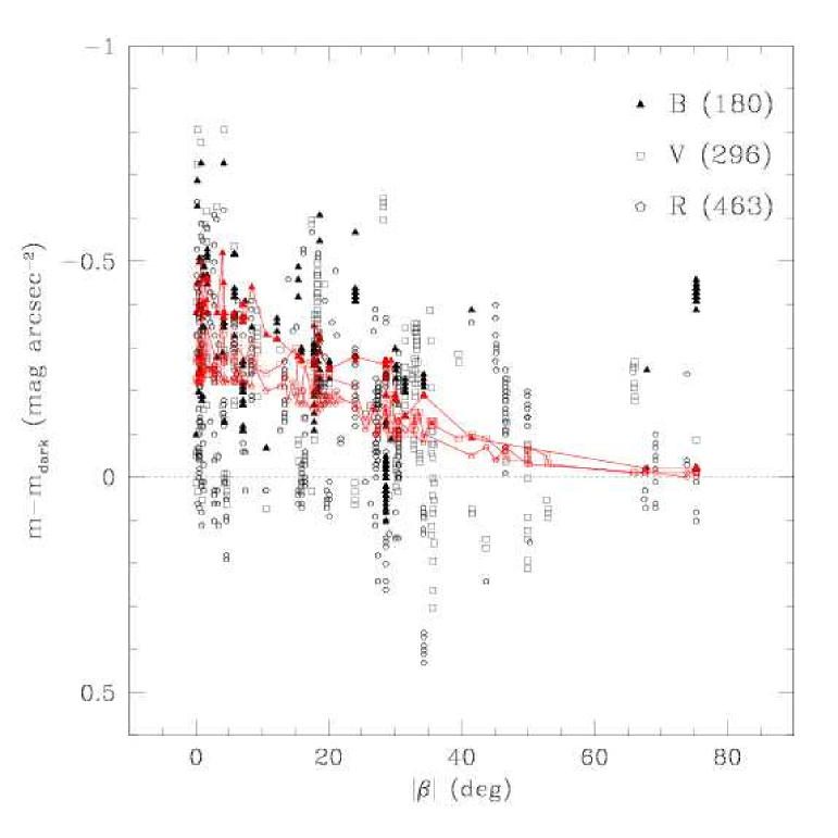
Figure 8: $B,V$ and $R$ dark time sky brightness variations as a function of ecliptic latitude. The solid lines trace the behaviour expected from Levasseur-Regourd & Dumont (levasseur (1980)) data for the different passbands.

6 Sky brightness variations during the night

In the literature one can find several and discordant results about the sky brightness variations as a function of the time distance from astronomical twilight. Walker (1988b ) first pointed out that the sky at zenith gets darker by $\sim$0.4 mag arcsec^-2 during the first six hours after the end of twilight. Pilachowski et al. (pila (1989)) found dramatic short time scale variations, while the steady variations were attributed to airmass effects only (see their Figure 2). This explanation looks indeed reasonable, since the observed sky brightening is in agreement with the predictions of Garstang (garstang89 (1989)). Krisciunas (1990, his Figure 6) found that his data obtained in the $V$ passband showed a decrease of $\sim$0.3 mag arcsec^-2 in the first six hours after the end of twilight, but he also remarked that this effect was not clearly seen in $B$. Due to the high artificial light pollution, Lockwood, Floyd & Thompson (lockwood (1990)) tend to attribute the nightly sky brightness decline they observe at the Lowell Observatory, to progressive reduction of commercial activity.

Walker’s findings were questioned by Leinert et al. (leinert95 (1995)) and Mattila et al. (attila (1996)), who state that no indications for systematic every-night behaviour of a decreasing sky brightness after the end of twilight were shown by their observations. Krisciunas (krisc97 (1997)) notes that, on average, the zenith sky brightness over Mauna Kea shows a not very convincing sky brightness change of 0.03 mag hour^-1. On the other hand he also reports cases where the darkening rate was as large as 0.24 mag hour^-1 and discusses the possibility of a reverse Walker effect taking place during a few hours before the beginning of morning twilight.

Leinert et al. (leinert98 (1998)) touch this topic in their extensive review, pointing out that this is an often observed effect due to a decreasing release rate of the energy stored in the atmospheric layers during day time. Finally, Benn & Ellison (benn (1998)) do not find any signature of steady sky brightness variation depending on the time distance from twilights at La Palma, and suggest that the effect observed by Walker is due to the variable contribution of the zodiacal light, a hypothesis already discussed by Garstang (garstang97 (1997)). A further revision of Walker’s findings is presented here in Appendix D, where we show that the effect is significantly milder than it was thought and probably influenced by a small number of well sampled nights.

We have performed an analogous analysis on our data set, using only the measurements obtained during dark time and correcting for differential zodiacal light contribution. Since the time range covered by our observations is relatively small with respect to the solar cycle, we do not expect the solar activity to play a relevant role, and hence we reckon it is reasonable not to normalise the measured sky brightness to some reference time. This operation would be anyway very difficult, due to the vast amount of data and the lack of long time series. The results are presented in Figure 9, where we have plotted the sky brightness vs. time from evening twilight, $\Delta t_{etwi}$, for $B,V,R$ and $I$ passbands. Our data do not support the exponential drop seen by Walker (1988b ) during the first 4 hours and confirm the findings by Leinert et al. (leinert95 (1995)), Mattila et al. (attila (1996)) and Benn & Ellison (benn (1998)). This is particularly true for $V$ and $R$ data, while in $B$ and especially in $I$ one might argue that some evidence of a rough trend is visible. As a matter of fact, a blind linear least squares fit in the range 0 $\leq\Delta t_{etwi}\leq$ 6 gives an average slope of 0.04$\pm$0.01 and 0.03$\pm$0.01 mag hour^-1 for the two passbands respectively. Both values are a factor of two smaller than those found by Walker (1988b ) but are consistent, within the quoted errors, with the values we found revising his original data (see Appendix D). However, the fact that no average steady decline is seen in $V$ and $R$ casts some doubt on the statistical significance of the results one gets from $B$ and $I$ data. This does not mean that on some nights very strong declines can be seen, as already pointed out by Krisciunas (krisc97 (1997)). Our data set includes several such examples, but probably the most interesting is the one which is shown in Figure 10, where we have plotted the data collected on five consecutive nights (2000 April 3–7). As one can see, the $I$ data (upper panel) show a clear common trend, even though segments with different slopes are present and the behaviour shown towards the end of the night during 2000 April 6 is opposite to that of 2000 April 5. This trend becomes less clear in the $R$ passband (middle panel) and it is definitely not visible in $V$ (lower panel), where the sky brightness remains practically constant for about 6 hours. Unfortunately, no $B$ data are available during these nights.

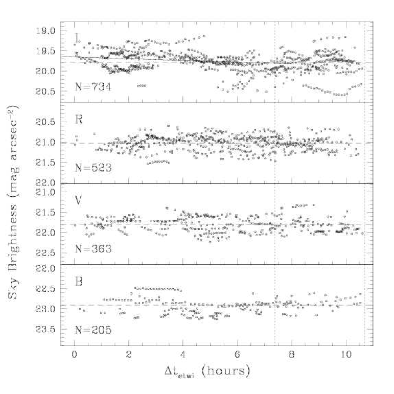
Figure 9: Dark time Paranal night sky brightness, corrected for zodiacal light contribution, as a function of time distance from evening twilight. The vertical dotted lines indicate the shortest and longest night (7.4 and 10.7 hours respectively, astronomical twilight to twilight), while the dashed horizontal line is placed at the average value in each passband.

A couple of counter-examples are shown in Figure 11: the upper and lower panels show two well sampled time series obtained on the same sky patch, which show that during those nights the sky brightness was roughly constant during the phase where the Walker effect is expected to be most efficiently at work. Instead of a steady decline, clear and smooth sinusoidal fluctuations with maximum amplitudes of $\sim$0.1 mag and time scales of the order of 0.5 hours are well visible. Finally, to show that even mixed behaviours can take place, in the central panel we have presented the $R$ data collected on 23-02-2001, when a number of different sky patches was observed. During that night, the sky brightness had a peak-to-peak fluctuation of $\sim$0.7 mag and showed a steady increase for at least 4 hours.

To conclude, we must say that we tend to agree with Leinert et al. (leinert95 (1995)) that the behaviour shown during single nights covers a wide variety of cases and that there is no clear average trend. We also add that mild time-dependent effects cannot be ruled out; they are probably masked by the much wider night-to-night fluctuations and possibly by the patchy nature of the night sky even during the same night.

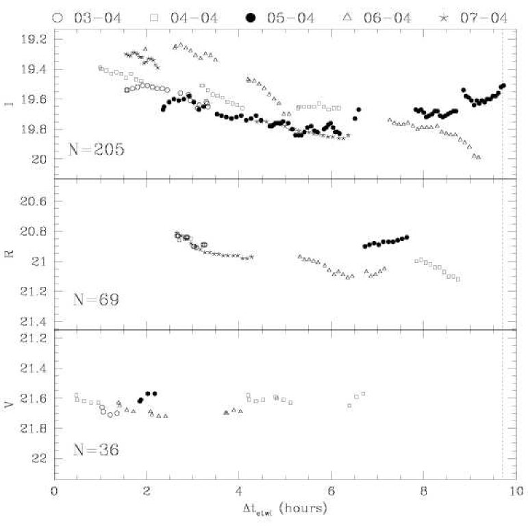
Figure 10: Time sequences collected on April 2–7, 2000. The data have been corrected for airmass and differential zodiacal light contribution. The vertical dotted line is placed at the beginning of morning astronomical twilight.

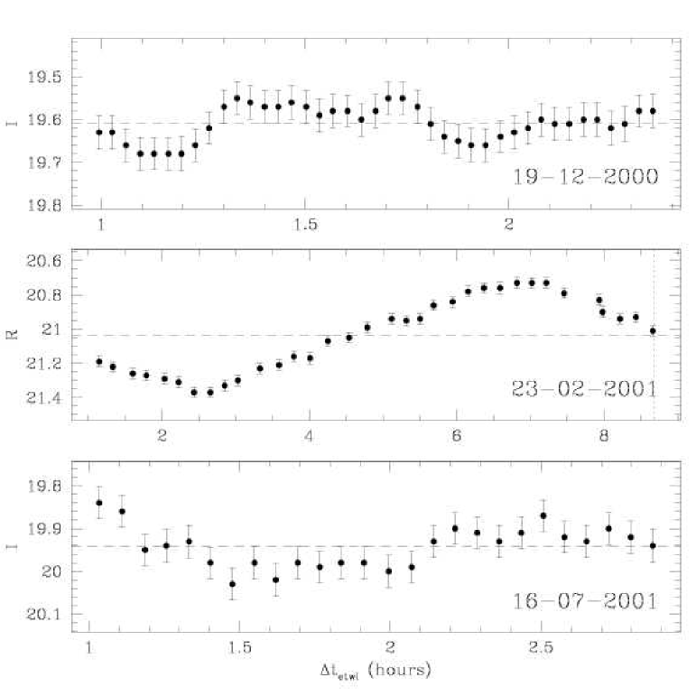
Figure 11: Time sequences collected on 19-12-2000 ($I$), 23-02-2001 ($R$) and 16-07-2001 ($I$). The data have been corrected for airmass and differential zodiacal light contribution. The vertical dotted line is placed at the beginning of morning astronomical twilight.

7 Testing the moon brightness model

As we have mentioned in Sec. 4.2, some data have been collected when the moon contribution to the sky brightness is conspicuous and this offers us the possibility of directly measuring its effect and comparing it with the model by Krisciunas & Schaefer (krischae (1991)) which, to our knowledge, is the only one available in the literature.

To estimate the fraction of sky brightness generated by scattered moon light, we have subtracted to the observed fluxes the average values reported in Table 4 for each passband. The results are presented in the lower panel of Figure 12, where we have plotted only those data for which the observed value was larger than the dark time one. As expected, the largest deviations are seen in $B$, where the sky brightness can increase by about 3 mag at 10 days after new moon, while in $I$, at roughly the same moon age, this deviation just reaches $\sim$1.2 mag. It is interesting to note that most exposure time calculators for modern instruments make use of the function published by Walker (walker87 (1987)) to compute the expected sky brightness as a function of moon age. As already noticed by Krisciunas (krisc90 (1990)), this gives rather optimistic estimates, real data being most of the time noticeably brighter. This is clearly visible in Figure 12, where we have overplotted Walker’s function for the $V$ passband to our data: already at 6 days past new moon the observed $V$ data (open squares) show maximum deviations of the order of 1 mag. These results are fully compatible with those presented by Krisciunas (krisc90 (1990)) in his Figure 8.

Another weak point of Walker’s function is that it has one input parameter only, namely the moon phase, and this is clearly not enough to predict with sufficient accuracy the sky brightness. This, in fact, depends on a number of parameters, some of which, of course, are known only when the time the target is going to be observed is known. In this respect, the model by Krisciunas & Schaefer (krischae (1991)) is much more promising, since it takes into account all relevant astronomical circumstances. The model accuracy was tested by the authors themselves, who reported RMS deviations as large as 23% in a brightness range which spans over 20 times the typical value observed during dark time.

In the upper panel of Figure 12 we have compared our results with the model predictions, including $B,V,R$ and $I$ data. We emphasise that we have used average values for the extinction coefficients and dark time sky brightness and this certainly has some impact on the computed values. On the other hand, this is the typical configuration under which the procedure would be implemented in an exposure time calculator, and hence it gives a realistic evaluation of the model practical accuracy. Figure 12 shows that, even if deviations as large as 0.4 mag are detected, the model gives a reasonable reproduction of the data in the brightness range covered by our observations. This is actually less than half with respect to the one encompassed by the data shown in Figure 3 of Krisciunas & Schaefer (krischae (1991)), which reach $\sim$8300 sbu in the $V$ band.

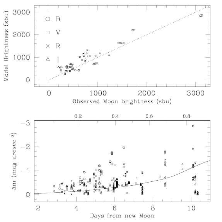
Figure 12: Lower panel: observed sky brightness variation as a function of moon age for $B,V,R$ and $I$. The solid line traces the data published by Walker (walker87 (1987)) for the $V$ passband while the upper scale shows the fractional lunar illumination. Upper panel: comparison between the observed and predicted moon contribution (Krisciunas & Schaefer krischae (1991)). Plotted are only those data points for which the global brightness is larger than the typical dark time brightness.

8 Sky brightness vs. solar activity

As we have mentioned in Sec. 4.3, during the time covered by the data presented here, the solar activity had probably reached its maximum. To be more precise, since the current solar cycle (n. 23) has a double peak structure (see Figure 6), our measurements cover the descent from the first maximum and the abrupt increase to the second maximum. Mainly due to the latter transition, the solar density flux at 10.7 cm in our data set ranges from 1.2 MJy to 2.4 MJy, the median value being 1.8 MJy. Even though this is almost half of the full range expected on a typical complete 11 years solar cycle (80$-$250 MJy), a clear variation is seen in the same solar density flux range from similar analysis performed by other authors (see for example Mattila et al. 1996, their Figure 6). In Figure 13 we show the case of the $R$ passband, where we have plotted the nightly average sky brightness vs. the solar density flux measured during the day immediately preceeding the observations. A linear least squares fit to the data (solid line) gives a slope of 0.14$\pm$0.01 mag arcsec^-2 MJy^-1, which turns into a variation of 0.24$\pm$0.11 mag arcsec^-2 during a full solar cycle. This value is a factor two smaller than what has been reported for $B$, $V$ (Walker 1988b, Krisciunas 1990) and $uvgyr$ (Leinert et al. 1995, Mattila et al. 1996) for yearly averages and it is consistent with a null variation at the 2 sigma level. Moreover, since the correlation factor computed for the data in Figure 13 is only 0.19, we think there is no clear indication for a real dependency.

This impression is confirmed by the fact that a similar analysis for the $B$ and $V$ passbands gives an extrapolated variation of 0.08$\pm$0.13 and 0.07$\pm$0.11 mag arcsec^-2 respectively. These numbers, which are consistent with zero, and the low correlation coefficients (0.08 and 0.11 respectively) seem to indicate no short–term dependency from the 10.7 cm solar flux. Similar values are found for the $I$ passband ($\Delta m$=0.22$\pm$0.15 mag arcsec^-2). These results agree with the findings by Leinert et al. (leinert95 (1995)) and Mattila et al. (attila (1996)) and the early work of Rosenberg & Zimmermann (rosenberg (1967)), who have shown that the [OI]5577Å line intensity correlates with the 2800MHz solar flux much more strongly using the monthly averages than the nightly averages. For all these reasons, we agree with Mattila et al. (attila (1996)) in saying that no firm prediction on the night sky brightness can be made on the basis of the solar flux measured during the day preceeding the observations, as it was initially suggested by Walker (1988b ). A possible physical explanation for this effect is that there is some inertia in the energy release from the layers ionised by the solar UV radiation, such that what counts is the integral over some typical time scale rather than the instantaneous energy input.

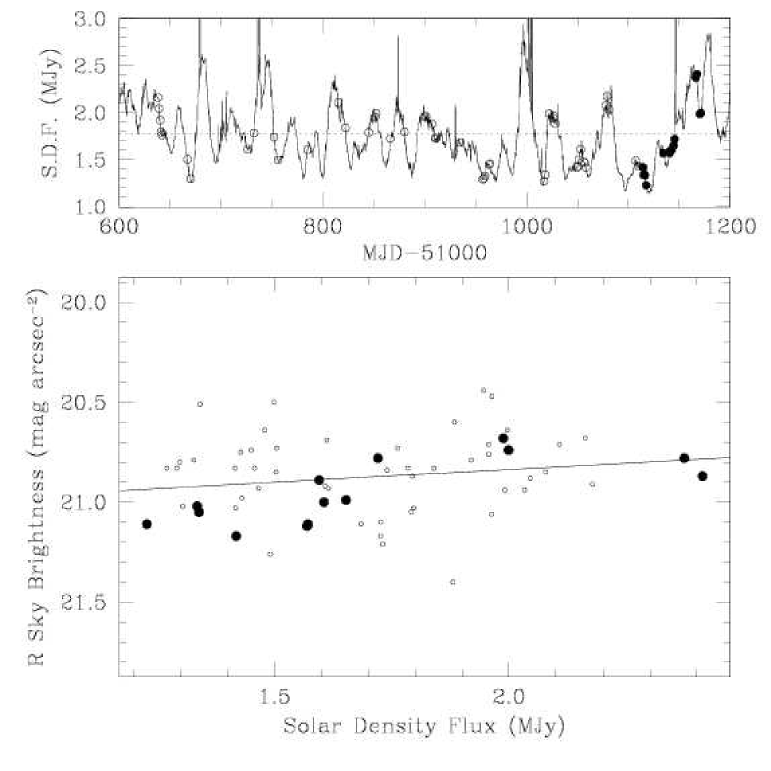
Figure 13: Lower panel: nightly average sky brightness in the $R$ passband vs. solar density flux. The filled circles represent data taken at MJD$>$52114, while the solid line indicates a linear least squares fit to all data. Upper panel: Penticton-Ottawa solar flux at 2800 MHz during the time interval discussed in this paper. The open circles indicate the values which correspond to the data presented in the lower panel and the dotted line is placed at the median value for the solar density flux.

9 Discussion and conclusions

Table 5: Dark time zenith night sky brightness measured at various observatories (adapted from Benn & Ellison 1998). $S_{10.7cm}$ is the Penticton-Ottawa solar density flux at 2800 MHz (Covington 1969).

Site	Year	$S_{10.7cm}$	$U$	$B$	$V$	$R$	$I$	Reference
		MJy	mag arcsec-2
La Silla	1978	1.5	-	22.8	21.7	20.8	19.5	Mattila et al. (1996)
Kitt Peak	1987	0.9	-	22.9	21.9	-	-	Pilachowski et al. (1989)
Cerro Tololo	1987-8	0.9	22.0	22.7	21.8	20.9	19.9	Walker (1987, 1988a)
Calar Alto	1990	2.0	22.2	22.6	21.5	20.6	18.7	Leinert et al. (1995)
La Palma	1994-6	0.8	22.0	22.7	21.9	21.0	20.0	Benn & Ellison (1998)
Mauna Kea	1995-6	0.8	-	22.8	21.9	-	-	Krisciunas (1997)
Paranal	2000-1	1.8	22.3	22.6	21.6	20.9	19.7	this work

Besides being the first systematic campaign of night sky brightness measurements at Cerro Paranal, the survey we have presented here has many properties that make it rather unique. First of all, the fact that it is completely automatic ensures that each single frame which passes through the quality checks contributes to build a continously growing sample. Furthermore, since the data are produced by a very large telescope, the measurements accuracy is quite high when compared to that generally achieved in this kind of study, which most of the time make use of small telescopes. Another important fact, related to both the large collecting area and the use of a CCD detector, is that the usual problem of faint unresolved stars is practically absent. In fact, with small telescopes, it is very difficult to avoid the inclusion of stars fainter than $V$=13 in the beam of the photoelectric photometer (see for example Walker 1988b). The contribution of such stars is 39.1 $S_{10}(V)$ (Roach & Gordon roachgordon (1973), Table 2-I) which corresponds to about 13% of the global sky brightness. Now, with the standard configuration and a seeing of 1^′′, during dark time FORS1 can reach a 5$\sigma$ peak limiting magnitude $V\simeq$23.3 in a 60 seconds exposure for unresolved objects. As the simulations show (see Patat patat (2002)), the algorithm we have adopted to estimate the sky background is practically undisturbed by the presence of such stars, unless their number is very large, a case which would be rejected anyway by the $\Delta$-test (Patat patat (2002)). Now, since the typical contribution of stars with $V\geq$20 is 3.2 $S_{10}(V)$ (Roach & Gordon roachgordon (1973)), we can conclude that the effect of faint unresolved stars on our measurements is less than 1%.

Another distinguishing feature is the time coverage. As reported by Benn & Ellison (benn (1998)), the large majority of published sky brightness measurements were carried out during a limited number of nights (see their Table 1). The only remarkable exception is represented by their own work, which made use of 427 CCD images collected on 63 nights in ten years. Nevertheless, this has to be compared with our survey which produced about 3900 measurements during the first 18 months of steady operation. This high time frequency allows one to carry out a detailed analysis of time dependent effects, as we have shown in Sec. 6 and to get statistically robust estimates of the typical dark time zenith sky brightness.

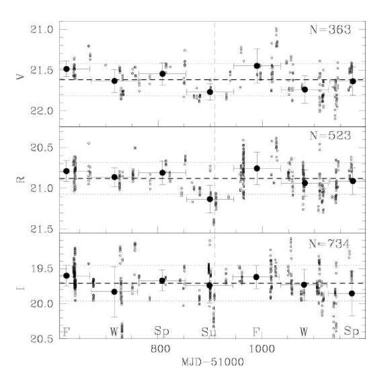
Figure 14: $V$, $R$ and $I$ (from top to bottom) dark time sky brightness measured at Paranal from April 2000 to September 2001. For each passband the average value (dashed line) and the $\pm$1$\sigma$ interval (dotted lines) are plotted. The large solid dots are placed at the seasonal average values computed within the time interval indicated by the horizontal error bars, while the vertical error bars represent the corresponding RMS sky brightness dispersion. The labels on the lower side indicate the austral astronomical season: winter (W), spring (Sp), summer (Su) and fall (F). The vertical dashed line indicates December 31, 2000.

The values we have obtained for Paranal are compared to those of other dark astronomical sites in Table 5. The first thing one notices is that the values for Cerro Paranal are very similar to those reported for La Silla, which were also obtained during a maximum of solar activity. They are also not very different from those of Calar Alto, obtained in a similar solar cycle phase, even though Paranal and La Silla are clearly darker in $R$ and definitely in $I$. All other sites presented in Table 5 have data which were obtained during solar minima and are therefore expected to show systematically lower sky brightness values. This is indeed the case. For example, the $V$ values measured at Paranal are about 0.3 mag brighter then those obtained at other sites at minimum solar activity (Kitt Peak, Cerro Tololo, La Palma and Mauna Kea). The same behaviour, even though somewhat less pronounced, is seen in $B$ and $I$, while it is much less obvious in $R$. Finally, the $U$ data show an inverse trend, in the sense that at those wavelengths the sky appears to be brighter at solar minima. Interestingly, a plot similar to that of Figure 13 also gives a negative slope, which turns into a variation $\Delta U$=$-$0.7$\pm$0.5 mag arcsec^-2 during a full solar cycle. Due to the rather large error and the small number of nights (11), we think that no firm conclusion can be drawn about a possible systematic effect, but we notice that a similar behaviour is found by Leinert et al. (leinert95 (1995)) for the $u$ passband (see their Figure 6). Since the airglow in $U$ is dominated by the O₂ Herzberg bands $A^{3}\Sigma-X^{3}\Sigma$ (Broadfoot & Kendall 1968), the fact that their intensity seems to decrease with an increasing ionising solar flux could probably give some information on the physical state of the emitting layers, where molecular oxygen is confined.

At any rate, the $BVRI$ Paranal sky brightness will probably decrease in the next 5-6 years, to reach its natural minimum around 2007. The expected darkening is of the order of 0.4-0.5 mag arcsec^-2 (Walker 1988b), but the direct measurements will give the exact values for this particular site. In the next years this survey will provide an unprecedented mapping of the dependency from solar activity. So far, in fact, this correlation has been investigated with sparse data, affected by a rather high spread due to the night-to-night variations of the airglow (see for instance Figure 4 by Krisciunas 1990), which tend to mask any other effect and make any conclusion rather uncertain.

As already pointed out by several authors, the night sky can vary significantly over different time scales, following physical processes that are not completely understood. As we have shown in the previous section, even the daily variations in the solar ionising radiation are not sufficient to account for the observed night-to-night fluctuations. Moreover, the observed scatter in the dark time sky brightness (see Sec. 5) is certainly not produced by the measurement accuracy and can be as large as 0.25 mag (RMS) in the $I$ passband; since the observed distribution is practically Gaussian (see Figure 7), this means that the $I$ sky brightness can range over $\sim$1.4 mag, even after removing the effects of airmass and zodiacal light contribution. This unpredictable variation has the unpleasant effect of causing maximum signal-to-noise changes of about a factor of 2.

Besides these short time scale fluctuations that we have discussed in Sec. 6 and the long term variation due to the solar cycle, one can reasonably expect some effects on intermediate time scales. With this respect we have computed the sky brightness values averaged over three months intervals, centered on solstices and equinoxes. The results for $V$, $R$ and $I$ are plotted in Figure 14, where we have used all the available data obtained at Paranal during dark time, with $\Delta_{twi}\geq$0. This figure shows that there is no convincing evidence for any seasonal effect, especially in the $I$ passband, where all three-monthly values are fully consistent with the global average (thick dashed line). The only marginal detection of a deviation from the overall trend is that seen in $R$ in correspondence of the austral summer of year 2000, when the average sky brightness turns out to be $\sim$1.3$\sigma$ fainter than the global average value. Even though a decrease of about 0.1 mag is indeed expected in the $R$ passband as a consequence of the NaI D flux variation (see Roach & Gordon roachgordon (1973) and the discussion below), we are not completely sure this is the real cause of the observed effect, both because of the low statistical significance and the fact that a similar, even though less pronounced drop, is seen at the same epoch in the $V$ band, where the NaI D line contribution is negligible (see Figure 1).

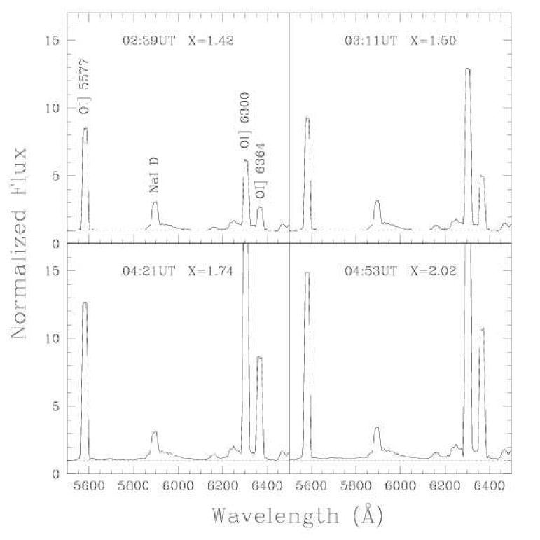
Figure 15: Evolution of the night sky spectrum on February 25, 2001 in the wavelength range 5500-6500 Å. The original 1800 seconds spectra were obtained with FORS1, using the standard resolution collimator and a long slit 1^′′ wide (see also the caption of Figure 1). In each panel the starting UT time and airmass $X$ are reported. For presentation the four spectra have been normalised to the continuum of the first one in the region 5600-5800 Å.

To illustrate how complex the night sky variations can be, we present a sequence of four spectra taken at Paranal during a moonless night in Figure 15, starting more than two hours after evening twilight with an airmass ranging from 1.4 to 2.0. For the sake of simplicity we concentrate on the spectral region 5500-6500Å, right at the intersection between $V$ and $R$ passbands, which contains the brightest optical emission lines and the so called pseudo-continuum (see Sec. 1). Due to the increasing airmass, the overall sky brightness is expected to grow according to Eq. 10, which for $V$ and $R$ gives a variation of about 0.2 mag. These values are in rough agreement with those one gets measuring the continuum variation at 5500Å (0.13 mag) and 6400Å (0.18 mag). Interestingly, this is not the case for the synthetic $V$ and $R$ magnitudes derived from the same spectra, which decrease by 0.32 and 0.51 mag respectively, i.e. much more than expected, specially in the $R$ band. This already tells us that the continuum and the emission lines must behave in a different manner. In fact, the flux carried by the [OI]5577Å line changes by a factor 1.9 from the first to the last spectrum, whereas the adjacent continuum grows only by a factor 1.1. For the NaI D lines, these two numbers are 1.4 and 1.2, still indicating a dichotomy between the pseudo-continuum and the emission lines. But the most striking behaviour is that displayed by the [OI]6300,6364Å doublet: the integrated flux changes by a factor 5.2 in about two hours and can be easily identified as the responsible for the brightening observed in the $R$ passband. This is easily visible in Figure 15, where the [OI]6300Å component surpasses the [OI]5577Å in the transition from the first to the second spectrum and keeps growing in intensity in the subsequent two spectra. The existence of these abrupt changes is known since the pioneering work by Barbier (barbier (1957)), who has shown that [OI]6300,6364Å can undergo strong brightness enhancements over an hour or two on two active regions about 20^∘ on either side of the geomagnetic equator, which roughly corresponds to tropical sites. With Cerro Paranal included in one of these active areas, such events are not unexpected. A possible physical explanation for this effect is described by Ingham (ingham (1972)), and involves the release of charged particles at the conjugate point of the ionosphere, which stream along the lines of force of the terrestrial magnetic field. We notice that in our example, the first spectrum was taken about two hours before local midnight, at about one month before the end of austral summer. This is in contrast with Ingham’s explanation, which implies that this phenomenon should take place in local winter, since in local summer the conjugate point, which for Paranal lies in the northern hemisphere, sees the sun later and not before, as it is the case during local winter.

Irrespective of the underlying physical mechanism, the [OI]6300,6364Å line intensity changed from 255 R to 1330 R; the fact that the initial value is definitely higher than that expected at these geomagnetic latitudes ($<$50 R, Roach & Gordon roachgordon (1973), Figure 4-12) seems to indicate that the line brightening had started before our first observation. On the other hand, the intensity of the [OI]5577Å line in the first spectrum is 220 R, i.e. well in agreement with the typical value (250 R, Schubert & Walterscheid 2000).

The case of NaI D lines is slightly different, since these features follow a strong seasonal variation which makes them brighter in winter and fainter in summer, the intensity range being 30-200 R (Schubert & Walterscheid 2000). This fluctuation is expected to produce a seasonal variation with an amplitude of about 0.1 mag in the $R$ passband, while in $V$ the effect is negligible. Actually, the minimum intensity of this feature can change from site to site, according to the amount of light pollution. In fact, most of the radiation produced by low-pressure sodium lamps is released through this transition. For example, Benn & Ellison (benn (1998)) report for La Palma an estimated artificial contribution to the Sodium D lines of about 70 R. In our first spectrum, the measured intensity is 73 R, a value which, together with the epoch when it was obtained (end of summer) and the relatively large airmass ($X$=1.5), indicates a very small contribution from artificial illumination. However, a firmer limit can be set analysing a large sample of low resolution spectra taken around midsummer, a task which is beyond the purpose of this paper.

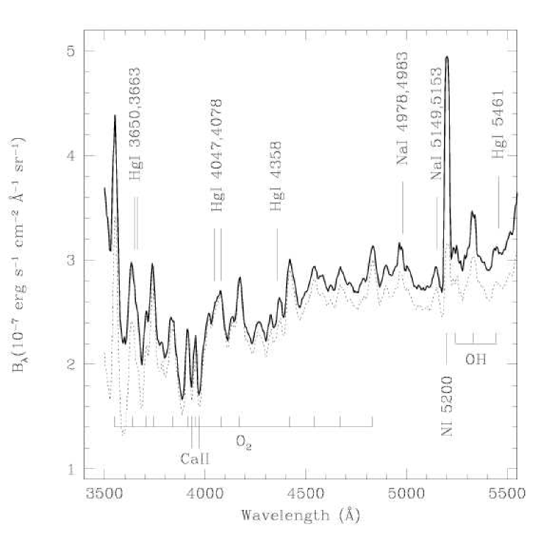
Figure 16: Night sky spectrum obtained at Paranal on February 25, 2002 at 04:53 UT (see Figure 15). Marked are the expected positions for the most common lines produced by artificial scattered light (upper ticks) and natural atmospheric features (lower ticks). The dotted line traces part of the spectrum taken during the same night at 02:39 UT.

To search for other possible signs of light pollution, we have examined the wavelength range 3500-5500Å of the last spectrum presented in Figure 15, which was obtained at a zenith distance of about 60^∘ and at an azimuth of 313^∘. A number of Hg and Na lines produced by street lamps, which are clearly detected at polluted sites, falls in this spectral region. As expected, there is no clear trace of such features in the examined spectrum; in particular, the strongest among these lines, HgI 4358Å, is definitely absent. This appears clearly in Figure 16, where we have plotted the relevant spectral region and the expected positions for the brightest Hg and Na lines (Osterbrock & Martel 1992). In the same figure we have also marked the positions of O₂ and OH main features. A comparison with the spectra presented by Broadfoot & Kendall (broadfoot (1968)) again confirms the absence of the HgI lines and shows that almost all features can be confidently identified with natural transitions of molecular oxygen and hydroxyl. There are probably two exceptions only, which happen to be observed very close to the expected positions for NaI 4978, 4983Å and NaI 5149, 5163Å, lines typically produced by high pressure sodium lamps (Benn & Ellison 1998). They are very weak, with an intensity smaller than 2 R, and their contribution to the broad band sky brightness is negligible. Nevertheless, if real, they could indicate the possible presence of some artificial component in the NaI D lines, which are typically much brighter. This can be verified with the analysis of a high resolution spectrum. If the contamination is really present, this should show up with the broad components which are a clear signature of high pressure sodium lamps. The inspection of a low airmass, high resolution (R=43000) and high signal-to-noise UVES spectrum of Paranal’s night sky (Hanuschik et al. 2003, in preparation) has shown no traces of neither such broad components nor of other NaI and HgI lines. For this purpose, suitable UVES observations at critical directions (Antofagasta, Yumbes mining plant) and high airmass periodically executed during technical nights, would probably allow one to detect much weaker traces of light pollution than any broad band photometric survey. But, in conclusion, there is no indication for any azimuth dependency in our dark time $UBVRI$ measurements.

There are finally two interesting features shown in Figure 16 which deserve a short discussion. The first is the presence of CaII H&K absorption lines, which are clearly visible also in the spectra presented by Broadfoot & Kendall (broadfoot (1968)) and are the probable result of sunlight scattered by interplanetary dust (Ingham 1962). This is not surprising, since the spectrum of Figure 16 was taken at $\beta$=$-$3^∘. 5 and $\lambda-\lambda_{\odot}$=139^∘. 8, i.e. in a region were the contribution from the zodiacal light is significant (see Figure 5). The other interesting aspect concerns the emission at about 5200Å. This unresolved feature, identified as NI, is extremely weak in the spectra of Broadfoot & Kendall (broadfoot (1968)), in agreement with its typical intensity (1 R, Roach & Gordon roachgordon (1973)). On the contrary, in our first spectrum (dotted line in Figure 16) it is very clearly detected at an intensity of 7.5 R and steadily grows until it reaches 32 R in the last spectrum, becoming the brightest feature in this wavelength range. This line, which is actually a blend of several very close NI transitions, is commonly seen in the Aurora spectrum with intensities of 0.1-2 kR (Schubert & Walterscheid 2000) and it is supposed to originate in a layer at 258 km. The fact that its observed growth (by a factor 4.3) follows closely the one we have discussed for [OI]6300,6364Å, suggests that the two regions probably undergo the same micro-auroral processes.

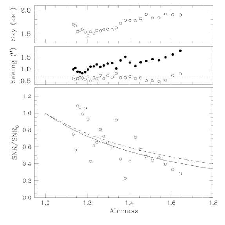
Figure 17: Lower panel: peak signal-to-noise ratio measured for the same star on a sequence of 150 seconds $I$ images obtained with FORS1 on July 16, 2001. Solid and dashed lines trace Eq. 3 for $U$ and $I$ passbands respectively. Middle panel: seeing measured by the Differential Image Motion Monitor (DIMM, Sandrock et al. 2000) at 5500 Å and reported to zenith (empty circles); each point represents the average of DIMM data over the exposure time of each image. The solid circles indicate the image quality (FWHM) directly measured on the images. Upper panel: sky background (in ke^-) measured on each image.

Such abrupt phenomena, which make the sky brightness variations during a given night rather unpredictable, are accompanied by more steady and well behaved variations, the most clear of them being the inherent brightening one faces going from small to large zenith distances. In fact, as we have seen, the sky brightness increases at higher airmasses, especially in the red passbands, where it can change by 0.4 mag going from zenith to airmass $X$=2. For a given object, as a result of the photon shot noise increase, this turns into a degradation of the signal-to-noise ratio by a factor 1.6, which could bring it below the detection limit. Unfortunately, there are two other effects which work in the same direction, i.e. the increase of atmospheric extinction and seeing degradation. While the former causes a decrement of the signal, the latter tends to dilute a stellar image on a larger number of pixels on the detector. Combining Eq. 10, the usual atmospheric extinction law $I=I_{0}\;10^{-0.4\kappa(X-1)}$ and the law which describes the variation of seeing with airmass ($s=s_{0}\;X^{0.6}$, Roddier 1981) we can try to estimate the overall effect on the expected signal-to-noise ratio at the central peak of a stellar object. After very simple calculations, one obtains the following expression:

$$\frac{SNR(X)}{SNR_{0}}=X^{-1.2}\;\left[(1-f)+fX\right]^{-\frac{1}{2}}\;10^{-0.2\kappa(X-1)}$$ (3)

where the 0 subscript denotes the zenith ($X$=1) value. Eq. 3 is plotted in Figure 17 for the two extreme cases, i.e. $U$ and $I$ passbands. For comparison, we have overplotted real measurements performed on a sequence of $I$ images obtained with FORS1 on July 16, 2001. Given the fact that the seeing was not constant during the sequence (see the central panel), Eq. 3 gives a fair description of the observed data, which show however a pretty large scatter. As one can see, the average SNR ratio decreased by about a factor of 2 passing from airmass 1.1 to airmass 1.6. Such degradation is not negligible, specially when one is working with targets close to the detection limit. For this reason we think that Eq. 3 could be implemented in the exposure time calculators together with the model by Krisciunas & Schaefer (krischae (1991)), to allow for a more accurate prediction of the effective outcome from an instrument. This can be particularly useful during service mode observations, when now-casting of sky conditions at target’s position is often required.

Appendix A Extinction Coefficients and Colour Terms

Extinction coefficients and colour terms were computed using the method outlined by Harris, Pim Fitzgerald & Cameron Reed (harris (1991)), i.e. via a single-step multi-linear least squares fit to the data provided by the observation of photometric standard star fields (Landolt 1992). This procedure, in fact, allows one to get the photometric solutions using different stars with suitable colour and airmass ranges, without the need for repeating the observations at different airmasses. Due to the FORS1 calibration plan implemented during the time range discussed in this work, this was a mandatory requirement. To get meaningful results, the method needs a fair number of stars well spread in colour and airmass. While the first requirement is almost always fulfilled for the Landolt fields suitable for CCD photometry, the second is more cumbersome to achieve using FORS1 data. In order to overcome this problem we have computed the photometric parameters on a bi-monthly basis, for those time ranges where at least 3 stars were observed at airmass larger than 1.6. Harris et al. (harris (1991)) recommend to use data spanning at least 1 airmass, but we had to relax this constraint in order to get a sufficient number of stars.

Table 6: Bi-monthly average extinction coefficients (mag airmass^-1) measured at ESO-Paranal with FORS1 during photometric nights. For each entry the total number of data points ($n$) and the number of data points with airmass larger than 1.6 ($n_{z}$) are reported. The last row of the table shows the weighted means and the corresponding RMS errors.

Time	U			B			V			R			I
Range	$\kappa$	$n$	$n_{z}$	$\kappa$	$n$	$n_{z}$	$\kappa$	$n$	$n_{z}$	$\kappa$	$n$	$n_{z}$	$\kappa$	$n$	$n_{z}$
03/04-00	0.41$\pm$0.05	87	3	-	-	-	0.11$\pm$0.02	120	4	-	-	-	0.07$\pm$0.02	88	8
05/06-00	-	-	-	0.25$\pm$0.01	43	3	0.09$\pm$0.01	47	4	0.07$\pm$0.01	46	4	-	-	-
07/08-00	0.47$\pm$0.01	122	12	0.23$\pm$0.01	132	14	0.11$\pm$0.01	162	19	0.07$\pm$0.01	151	15	0.05$\pm$0.01	138	19
11/12-00	0.43$\pm$0.01	78	9	0.21$\pm$0.01	86	16	0.11$\pm$0.01	89	13	0.07$\pm$0.01	83	14	0.03$\pm$0.01	85	10
01/02-01	0.45$\pm$0.02	122	24	0.22$\pm$0.02	154	29	0.10$\pm$0.01	163	33	0.07$\pm$0.01	148	28	0.04$\pm$0.01	145	29
05/06-01	0.40$\pm$0.03	64	4	0.19$\pm$0.02	66	4	0.09$\pm$0.01	60	3	0.06$\pm$0.01	60	3	0.01$\pm$0.01	68	3
07/08-01	0.43$\pm$0.02	117	18	0.22$\pm$0.01	139	17	0.12$\pm$0.01	143	20	0.08$\pm$0.01	124	17	0.04$\pm$0.01	68	17
09/10-01	0.44$\pm$0.02	125	3	0.24$\pm$0.01	143	3	0.11$\pm$0.01	141	4	0.08$\pm$0.01	120	4	0.06$\pm$0.01	130	5
	0.43$\pm$0.02			0.22$\pm$0.02			0.11$\pm$0.01			0.07$\pm$0.01			0.05$\pm$0.02

Some tests have shown that the available photometric data do not allow the computation of the second order colour term and extinction coefficient, which are usually included in the photoelectric photometry solutions (see Harris et al. 1991, their Eqs. 2.9). In fact, the introduction of such terms in the fitting of our data produces random oscillations in the solutions without any significant decrease in the variance. Both second order coefficients are accompanied by large errors and are always consistent with zero. This clearly means that the accuracy of our measurements is not sufficient to go beyond the first order term. For this reason, we have adopted $M-m=m_{0}+\gamma\times C\;-\kappa\times z$ as fitting function for the generic passband, where $M$ and $m$ are respectively the catalogue and instrumental magnitudes of the standard stars, $m_{0}$ is the zeropoint, $\gamma$ is the colour term with respect to some colour $C$, $\kappa$ is the extinction coefficient and $z$ is the airmass. To eliminate clearly deviating measurements, we have computed the photometric solutions in two steps. We have first used all data to get a starting guess from which we have computed the global RMS deviation $\sigma$. Then we have rejected all data deviating more than 1.5$\times\sigma$ and performed again the least squares fit on the selected data.

The results for the extinction coefficients are presented in Table 6. For each time range and passband we have reported the best fit value of $\kappa$, the estimated RMS error (both in mag airmass^-1) and the number of data points used for the least squares fit.

The values of $\kappa$ in the various bands show some minor fluctuations. Of course, we cannot exclude night-to-night variations, which are clearly observed at other sites (see for instance Krisciunas 1990). This would require a dedicated monitoring, which is beyond the scope of this work and not feasible with the available data. Here we can only conclude that, on average, the extinction coefficients do not show any significant evolution or clear seasonal effects during the 20 months covered by the data discussed in this paper. Therefore, given also the purpose of this analysis, we have assumed that the extinction coefficients are constant in time and equal to the average values reported on the last row of Table 6.

The computed colour terms are shown Table 7. We note that in those cases where the constraints on the airmass range and the number of data-points were not fulfilled, we have performed the best fit keeping $\kappa$ constant and equal to the average values given in Table 6. This prevented the best fit from giving results with no physical meaning due to the poor airmass coverage. As in the case of the extinction coefficients, the color terms show fluctuations which are within the errors, stronger oscillations being seen in the $U$ passband, where the accuracy of the photometry is lower.

On the basis of these results we can conclude that there are no strong indications for significant colour term evolution and it is therefore reasonable to assume that they are constant in time. For our purposes we have adopted the weighted mean values shown in the last row of Table 7.

Table 7: Bi-monthly average colour terms for FORS1. The total number of used data points are the same reported in Table 6, while the estimated RMS uncertainty on each entry is $0.01$. The last row shows the weighted mean values and their estimated RMS errors.

Time Range	$\gamma_{U-B}^{U}$	$\gamma_{B-V}^{B}$	$\gamma_{B-V}^{V}$	$\gamma_{V-R}^{R}$	$\gamma_{V-I}^{I}$
03/04-00	0.09	$-$0.07	0.04	0.02	$-$0.05
05/06-00	0.08	$-$0.08	0.04	0.02	$-$0.04
07/08-00	0.10	$-$0.08	0.03	0.00	$-$0.05
09/10-00	0.08	$-$0.07	0.05	0.04	$-$0.04
11/12-00	0.04	$-$0.09	0.04	0.04	$-$0.04
01/02-01	0.07	$-$0.08	0.03	0.03	$-$0.05
03/04-01	0.07	$-$0.08	0.04	0.03	$-$0.04
05/06-01	0.03	$-$0.09	0.05	0.02	$-$0.04
07/08-01	0.10	$-$0.08	0.03	0.02	$-$0.05
09/10-01	0.08	$-$0.08	0.04	0.04	$-$0.03
	0.07$\pm$0.02	$-$0.08$\pm$0.01	0.04$\pm$0.01	0.03$\pm$0.01	$-$0.04$\pm$0.01

Appendix B Sky brightness units

Throughout this paper we have expressed the sky brightness in mag arcsec^-2. Since other authors have used different units, we derive here the conversions for the most used ones. In the $cgs$ system, the sky brightness is expressed in erg s^-1 cm^-2 Å^-1 sr^-1. Now, if $m_{sky,\lambda}$ is the sky brightness in a given passband (in mag arcsec^-2) and $m_{0,\lambda}$ is the photometric system zeropoint of that passband, the conversion is obtained as follows:

$$B_{\lambda}(cgs)=10^{-0.4(m_{sky,\lambda}-m_{0,\lambda}-26.573)}$$ (4)

where the constant in the exponent accounts for the fact that 1 arcsec² corresponds to 2.35$\times$10^-11 sr. For example, if we use the constant $m_{0}$ for the Johnson system $V$ band given by Drilling & Landolt (drilling (2000)), for a typical night sky brightness $m_{sky,V}$=21.6 mag arcsec^-2, this gives $B_{V}\simeq$3.7$\times$10^-7 erg s^-1 cm^-2 Å^-1 sr^-1. For practical reasons, we have introduced the surface brightness unit sbu (see Sec. 4), which is defined as 1 sbu$\equiv$10^-9 erg s^-1 cm^-2 Å^-1 sr^-1. With this setting, the typical $V$ sky brightness is 366 sbu.

Often $B_{\lambda}$ is expressed in $SI$ units. The conversion from $cgs$ units is simple, since 1 erg s^-1 cm^-2 Å^-1 sr^-1$\equiv$ 10 W m^-2 sr^-1 $\mu$m^-1 and hence:

$$B_{\lambda}(SI)=10^{-0.4(m_{sky,\lambda}-m_{0,\lambda}-29.073)}$$ (5)

so that the typical $V$ sky brightness turns out to be 3.7$\times$10^-6 W m^-2 sr^-1 $\mu$m^-1.

Especially in the past, the sky brightness was expressed in $S_{10}$, which is defined as the number of 10^th magnitude stars per square degree required to produce a global brightness equal to the one observed in the given passband. Since 1 sr corresponds to 3.282$\times$10³ square degrees, the conversion is given by the following equation:

$$1\;S_{10}(\lambda)=10^{-0.4(1.21-m_{0,\lambda})}\;\;\mbox{erg s${}^{-1}$ cm${}^{-2}$ \AA${}^{-1}$ sr${}^{-1}$}$$ (6)

Again, using the constant given by Drilling & Landolt (drilling (2000)) for the $V$ band, one obtains $1\;S_{10}(V)\equiv$1.24$\times$10^-9 erg s^-1 cm^-2 Å^-1 sr^-1 $\equiv$ 1.24 sbu. For $U$, $B$, $R$ and $I$ the multiplicative constant is 1.38, 2.11, 0.57 and 0.28, respectively. Therefore, the sky brightness expressed in $S_{10}$ and in sbu are of the same order of magnitude in all optical broad bands. For example, the typical $V$ sky brightness is 295 $S_{10}(V)$.

Another unit used in the past is the nanoLambert (nL), which measures the perceived surface brightness and corresponds to 3.80 $S_{10}(V)$. For the $V$ passband this gives also $1\;nL\equiv 4.72$ sbu.

Finally, to quantify the intensity of night sky emission lines, the Rayleigh (R) unit is commonly adopted. It is defined as 10⁶/4$\pi$ photons s^-1 cm^-2 sr^-1 and the conversion from erg s^-1 cm ^-2 sr^-1 is given by the following expression:

$$1R\equiv 634.4\;\lambda\;\mbox{erg s${}^{-1}$ cm${}^{-2}$ sr${}^{-1}$}$$ (7)

where $\lambda$ is expressed in Å. The intensity of non-monochromatic features, like the pseudo-continuum, is generally expressed in R Å^-1.

For a more thorough discussion of the sky brightness units the reader is referred to Leinert et al. (leinert98 (1998)) and Benn & Ellison (benn (1998)).

Appendix C Airmass dependency

The results obtained by Garstang (garstang89 (1989)) can be used to derive an approximate expression for the sky brightness dependency on the zenith distance, as already pointed out by Krisciunas & Schaefer (krischae (1991)). If we assume that a fraction $f$ of the total sky brightness is generated by the airglow and the remaining $(1-f)$ fraction is produced outside the atmosphere (hence including zodiacal light, faint stars and galaxies), Garstang’s Eq. 29 can be rewritten in a more general way as follows:

$$b(Z)=b_{0}\;[(1-f)+f\;X)]$$ (8)

where $X$, the optical pathlength along a line of sight, is given by

$$X=(1-0.96\;sin^{2}Z)^{-1/2}$$ (9)

$Z$ being the zenith distance. For the hypothesis on which this result is based, the reader is referred to Garstang’s original pubblication and to the analysis presented by Roach & Meinel (roach (1955)). Here we just recall that Eqs. 8 and 9 were obtained assuming that the extra-terrestrial fraction $(1-f)$ comes from infinity, while the airglow emission is generated in a layer (the so called van Rhjin layer) placed at 130 km from the Earth’s surface.

While the intensity of the extra-terrestrial component is independent on the zenith distance, this is not true for the airglow, due to the variable depth of the emitting layer along the line of sight. This is taken into account by the term $X$, which grows towards the horizon.

In his model Garstang (garstang89 (1989)) considers three different mechanisms for the background light to reach the observer once it leaves the van Rhjin layer: direct transmission, aerosol scattering and Rayleigh scattering. As a matter of fact, the first channel dominates on the others (see Figure 5 in Garstang 1989) which, in a first approximation, can be safely neglected. One is therefore left with the propagation of the sky background light across the lower atmosphere, which is described by Garstang’s Eq. 30 through the extinction factor $EF$. Now, if $\kappa$ is the extinction coefficient for a given passband (in mag airmass^-1), we can write $EF\simeq 10^{-0.4\;(X-1)}$, so that the expected change in the sky brightness as a function of $X$ is given by:

$$\Delta m=-2.5\;log[(1-f)+f\;X]+\kappa\;(X-1)$$ (10)

We notice that using $f$=1 in this equation gives Eq. 2 of Krisciunas & Schaefer (krischae (1991)), which gives slightly larger values for $\Delta m$ than Eq. 10.

The expected behaviour is plotted in Figure 18, where we present the predicted sky brightness (upper panel) and sky colour variations (lower panel) for the different passbands. For $f$ we have assumed a typical value of 0.6 (see Garstang 1989 and Benn & Ellison 1998). As one can see the correction becomes relevant for$Z\geq$30^∘ and reaches values as large as $\sim$0.4 mag at $Z$=60^∘ (see also Table 8). These predictions are consistent with the measurements obtained by Pilachowski et al. (pila (1989)), Mattila et al. (attila (1996)), Leinert et al. (leinert95 (1995)) and Benn & Ellison (benn (1998)). In particular, Pilachowski et al. (pila (1989)) have clearly detected the sky inherent reddening (see their Figure 3), which is in fair agreement with the predictions of Eq. 10 for the $(B-V)$ colour (see also Figure 18, lower panel).

Table 8: Zenith corrections (mag) computed according to Eq. 10. The values have been calculated using Paranal average extinction coefficients $\kappa$ (see Tab 6) and $f$=0.6. The zenith distance $Z$ is expressed in degrees, while $X$ is in airmasses.

$Z$	$X$	$\Delta U$	$\Delta B$	$\Delta V$	$\Delta R$	$\Delta I$
10.0	1.01	0.00	0.01	0.01	0.01	0.01
20.0	1.06	0.01	0.03	0.03	0.03	0.04
30.0	1.15	0.03	0.06	0.08	0.08	0.08
40.0	1.29	0.05	0.11	0.14	0.15	0.16
50.0	1.51	0.07	0.18	0.24	0.26	0.27
60.0	1.89	0.08	0.27	0.37	0.40	0.42

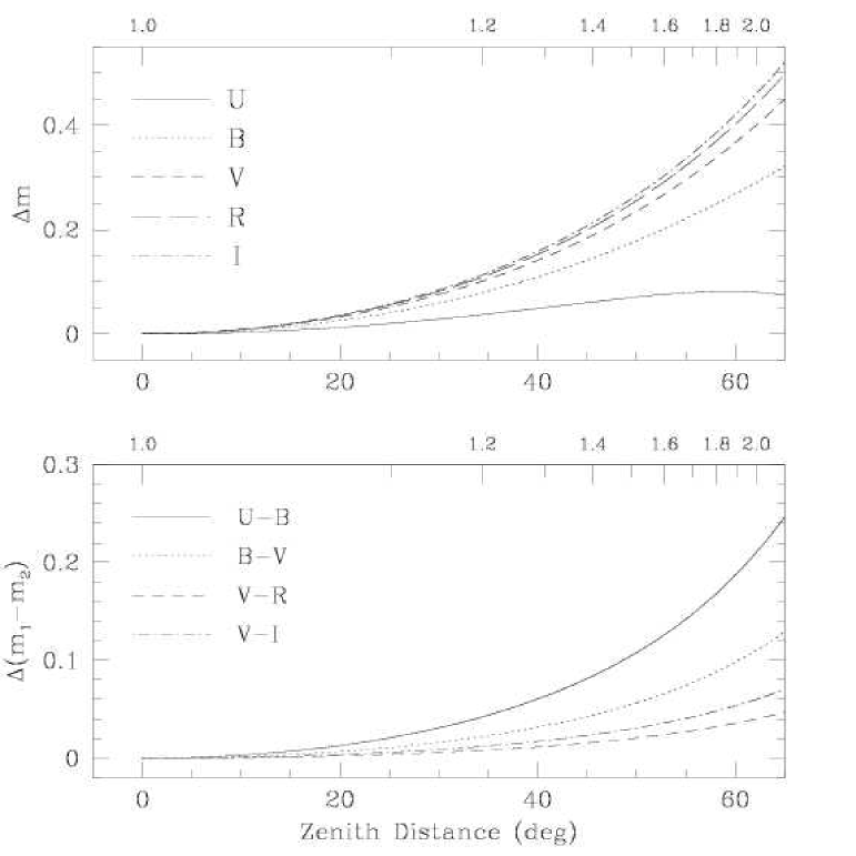
Figure 18: Upper panel: sky brightness variation (in mag arcsec^-2) as a function of zenith distance expected from Eq. 10 for $f$=0.6. For each passband the mean Paranal extinction coefficients presented in Table 6 were adopted. Lower panel: expected colour variation as a function of zenith distance. In both plots the upper scale reports the optical pathlength $X$, expressed in airmasses.

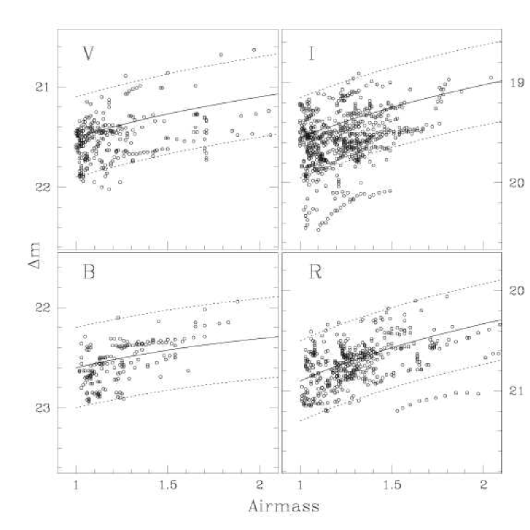
Figure 19: $B,V,R$ and $I$ sky brightness during dark time as a function of airmass. The solid line traces Eq. 10, while the dotted lines are placed at $\pm$0.4 mag from this law.

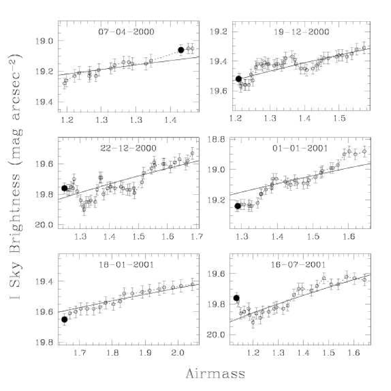
Figure 20: Sky brightness sequences on six different moonless nights at Paranal in the $I$ passband, corrected for zodiacal light contribution. The dotted line connects chronologically the various data points, while the filled dot indicates the first observation in each time series. Finally, the solid line traces Eq. 10 with $f$=0.7.

Our data confirm these findings, as it is shown in Figure 19, where we have plotted Paranal dark time measurements for $B,V,R$ and $I$ passbands. Even though the scattering due to night to night variations is quite large, the overall trend is consistent with the predictions of Eq. 10. The $U$ data, which reach airmass $X$=1.36 only, do not show a clear sky brightness increase, and this is again compatible with the expected value ($\sim$0.05 mag).

The airmass dependency is better visible when considering data obtained during single nights, when the overall sky brightness is reasonably stable. This is illustrated in Figure 20, where we present six very good series all obtained in the $I$ passband during moonless nights at Paranal. For comparison, we have plotted Eq. 10 with $f$=0.7, which reproduces fairly well the observed trend from airmass 1.2 to 2.0. As one can see, smooth deviations with peak values of $\sim$0.1 mag arcsec^-1 are detected within each single night, while the range spanned by the zenith extrapolated values is as large as $\sim$0.7 mag. The fact that a comparably large dispersion is seen in the other filters (see. Figure 18) suggests that night-to-night variations of this amplitude are common to all optical passbands.

We note that on April 7, 2000 and January 1, 2001 the observed slope was higher than predicted by Eq. 10. This implies that the contribution by the airglow to the global sky brightness in those nights was probably larger than the value we have used here, i.e. 70%. This hypothesis is in agreement with the fact that on 07-04-2000 and 01-01-2001 the extrapolated zenith value was 0.4$-$0.5 mag brighter than in all other nights shown in Figure 20.

Appendix D The Walker effect revisited

In this section we discuss and re-examine the findings published by Walker (1988b ). In Figure 21 we have plotted the $B$ data of his Table 1, with the exception of July 8, 1980 and May 4, 1984 (since they cover a very small time range with 2 and 3 points only) and the two data points marked by Walker with an asterisk in the sequences of May 11, 1983 and Apr 28, 1987. As one can see, there are only two dates in which a clear decreasing trend is visible, i.e. May 11, 1986 and April 25, 1987. Linear squares fitting to the two data sets give slopes of $\sim$0.08 $\pm$0.02 mag hour^-1 both in $B$ and $V$ filters, which turn into a sky brightness decrease of 0.48$\pm$0.12 mag during the first 6 hours of the night. Since Walker’s data have been collected across a full sunspot cycle, possible systematic variations due to the solar activity have to be removed. This can be achieved shifting all time sequences in order to have the same sky brightness at some reference time, an operation that also has the effect of correcting for night-to-night variations in the overall sky brightness. For this purpose we have performed, for each date, a linear least squares fit to the data and we have interpolated the resulting straight line at a time distance from the evening twilight $\Delta t_{etwi}$=2 hours. We note that a similar procedure must have been followed by Walker (1988b ), since in his Figure 2 all measurements refer to the magnitude at the end of evening twilight ($\Delta t_{etwi}$=0). Even though not explicitly mentioned in the paper, this implies that some extra/interpolation had to be performed, since estimates at $\Delta t_{etwi}$=0 are practically never available.

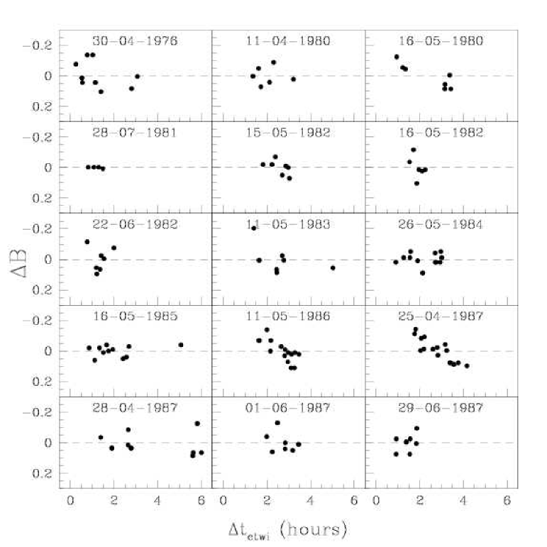
Figure 21: Zenith sky brightness at San Benito Mountain in the $B$ passband from Walker (1988b ). For clarity, the mean sky brightness has been subtracted to each time series.

To avoid meaningless extrapolations we have disregarded the data from July 28, 1981, which do not cover a suitable time range. Following Walker, we also have not included the data obtained in 1982, since they were most likely affected by the Chinchonal volcano eruption. Finally, to account for the differential contribution of zodiacal light, we have corrected Walker’s measurements using the data by Levasseur-Regourd & Dumont (levasseur (1980)) and assuming that all observations were carried out at the zenith of the observing site. The results one obtains following this procedure are presented in Figure 22, which shows a much less convincing evidence for a systematic trend than Walker’s Figure 2. In that case in fact, a decrement of $\sim$0.4 mag is seen during the first four hours, a behaviour which is definitely not visible in our Figure 22. As a matter of fact, a linear least squares fitting gives a rate of 0.02$\pm$0.01 and 0.03$\pm$0.01 mag hour^-1 for $B$ and $V$ respectively, which reduce to 0.01$\pm$0.01 and 0.02 $\pm$0.01 mag hour^-1 if one excludes the two sequences of May 11, 1986 and April 25, 1987 (empty circles). From these values we can deduce a maximum decrement of 0.1 and 0.2 mag in $B$ and $V$ respectively during the first 6 hours after the end of twilight. Therefore, our conclusion is that even though there is an indication for a systematic trend in Walker’s data, the rate is significantly lower than was thought. Moreover, due to the limited number of nights and the small time coverage of several of the time series, the results one gets may depend on the behaviour recorded during a few well sampled nights. For example, all data at $\Delta t_{etwi}>$5.5 hours were collected on April 28, 1987. This could explain why no other author has found the same strong effect when using larger data bases (see for instance Figure 9 of Benn & Ellison 1998).

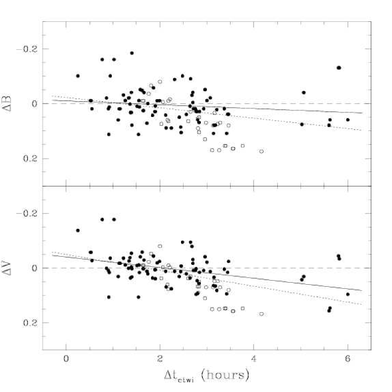
Figure 22: Variation in zenith sky brightness at San Benito Mountain with time after the end of astronomical twilight. Data have been corrected for differential zodiacal light contribution and all time series were normalised to the interpolated brightness at $\Delta t_{etwi}=2$ hours. Dotted and solid lines trace a linear least squares fitting with and without the data of May 11, 1986 and April 25, 1987 respectively (empty circles). Data are from Walker (1988b ).

References

- (1) Barbier, D. 1957, Compt. Rend. 244, 1945
- (2) Benn, C. R. & Ellison, S. L. 1998, La Palma Technical Note n.115
- (3) Broadfoot, A.L. & Kendall, K.R. 1968, J. Geophys. Res., 73, 426
- (4) Covington, A. E. 1969, JRASC, 63, 125
- (5) Drilling, J. S. & Landolt, A. U. 2000, in Allen’s astrophysical quantities, New York: AIP Press; Springer, 4th edition, Cox A. N. Ed.
- (6) Garstang, R. H. 1989, PASP, 101, 306
- (7) Garstang, R. H. 1997, BAAS, 29, 782
- (8) Hamuy, M., Walker, A.R., Suntzeff, N.B., et al. 1992, PASP, 104, 533
- (9) Harris, W.E., Pim Fitzgerald, M. & Cameron Reed, B. 1981, PASP, 93, 507
- (10) Huber, P. J. 1981, Robust statistics, John Wiley & Sons, p. 107
- (11) Ingham, M.F. 1962, MNRAS, 124, 505
- (12) Ingham, M.F. 1972, Sc. American, January 1972, p.78
- (13) Krisciunas, K. 1990, PASP, 102, 1052
- (14) Krisciunas, K. 1997, PASP, 109, 1181
- (15) Krisciunas, K. & Schaefer, B. E. 1991, PASP, 103, 1033
- (16) Landolt, A. U. 1992, AJ, 104, 340
- (17) Leinert, Ch., Väisanen, P., Mattila, K. & Lehtinen, K. 1995, A&AS, 112, 99
- (18) Leinert, Ch., Bowyer, S., Haikala, L.K., et al. 1998, A&AS, 127, 1
- (19) Levasseur-Regourd, A. C. & Dumont, R. 1980, A&A, 84, 277
- (20) Livingston, W. C. 2000, in Allen’s astrophysical quantities, New York: AIP Press; Springer, 4th edition, Cox A. N. Ed.
- (21) Lockwood, G. W., Floyd, R. D. & Thompson, D. T. 1990, PASP, 102, 481
- (22) Mattila, K., Väisänen, P. & Appen-Schnurr, G. F. O. 1996, A&AS, 119, 153
- (23) Meinel, A.B. 1950, ApJ, 111, 433
- (24) O’Connel, R. W. 1987, AJ, 94, 876
- (25) Osterbrock, D.E. & Martel, A. 1992, PASP, 104, 76
- (26) Patat, F. 2002, A&A, submitted
- (27) Pilachowski, C. A., Africano, J. L., Goodrich. B. D. & Binkert, W. S. 1989, PASP, 101, 707
- (28) Rayleigh, L. 1928, Proc. Roy. Soc. London, Ser. A, 119, 11
- (29) Roach, F. E. & Meinel, A. B. 1955, ApJ, 122, 554
- (30) Roach, F.E. & Gordon, J.L. 1973, The light of the Night Sky, D. Reidel Publ. Company, Dordrecht
- (31) Roddier, F. 1981, Progress in Optics, Vol. XIX, E. Wolf Ed.
- (32) Rosenberg, N. & Zimmerman. S.P. 1967, Planet. Space Sci. 15, 863
- (33) Sandrock, S., Amestica, R., Duhoux, P., Navarrete, J. & Sarazin, M. 2000, in Advanced Telescope and Instrumentation Control Software, Proc. SPIE 4009, 338, Hilton Lewis Ed.
- (34) Schaefer, B. E. 1998, S&T, May 1998, p.57
- (35) Schubert, G. & Walterscheid, R.L. 2000, in Allen’s astrophysical quantities, New York: AIP Press; Springer, 4th edition, Cox A.N. Ed., p.239
- (36) Szeifert, T. 2002, FORS1+2 User’s Manual, VLT-MAN-ESO-13100-1543, Issue 2.3
- (37) Walker, A. 1987, N.O.A.O. Newsletter, No. 10, 16
- (38) Walker, A. 1988, N.O.A.O. Newsletter, No. 13, 22
- (39) Walker, M. F. 1988, PASP, 100, 496