The power spectrum of galaxy clustering in the APM Survey

Abstract

We measure the power spectrum of galaxy clustering in real space from the APM Galaxy Survey. We present an improved technique for the numerical inversion of Limber’s equation that relates the angular clustering of galaxies to an integral over the power spectrum in three dimensions. Our approach is underpinned by a large ensemble of mock galaxy catalogues constructed from the Hubble Volume N-body simulations. The mock catalogues are used to test for systematic effects in the inversion algorithm and to estimate the errors on our measurement. We find that we can recover the power spectrum to an accuracy of better than $15\%$ over three decades in wavenumber. A key advantage of the use of mock catalogues to infer errors is that we can apply our technique on scales for which the density fluctuations are not Gaussian, thus probing the regime that offers the best constraints on models of galaxy formation. On large scales, our measurement of the power spectrum is consistent with the shape of the mass power spectrum in the popular “concordance” cold dark matter model. The galaxy power spectrum on small scales is strongly affected by nonlinear evolution of density fluctuations, and, to a lesser degree, by galaxy bias. The rms variance in the galaxy distribution, when smoothed in spheres of radius $8h^{-1}$Mpc, is $\sigma^{g}_{8}=0.96^{+0.17}_{-0.20}$ and the shape of the power spectrum on large scales is described by a simple fitting formula with parameter $\Gamma=0.19^{+0.13}_{-0.04}$ (these errors are the $1\sigma$ ranges for a two parameter fit). We use our measurement of the power spectrum to estimate the galaxy two point correlation function; the results are well described by a power law with correlation length $r_{0}=5.9\pm 0.7h^{-1}$Mpc and slope $\gamma=1.61\pm 0.06$ for pair separations in the range $0.1<r/(h^{-1}{\rm Mpc})<20$.

1 Introduction

The power spectrum of galaxy clustering is the equivalent of the Rosetta stone for structure formation in the Universe. On large scales, the power spectrum is a fossil record of the density fluctuations present at the epoch of recombination. Moving to intermediate and small scales, the spectrum encodes a wealth of information about different physical processes and effects: the nonlinear evolution of the density field, the modulation of the clustering signal of galaxies relative to that of the underlying dark matter, and, if the spectrum is estimated using the positions of galaxies inferred from their redshifts, the magnitude of peculiar motions and bulk flows.

In the past decade, significant progress has been made in measuring the power spectrum of galaxy clustering. Two main approaches have been taken: direct estimation in three dimensions using galaxy redshift surveys (e.g. Tadros & Efstathiou 1996; Hoyle et al. 1999; Sutherland et al. 1999; Percival et al. 2001) and the deprojection of angular clustering (e.g. Peacock 1991; Baugh & Efstathiou 1993, 1994a). Until the advent of the PSCz (Saunders et al. 2000) and 2dF Galaxy Redshift Survey (2dFGRS, Colless et al. 2001), angular catalogues (e.g. the APM Survey described by Maddox, Efstathiou & Sutherland, 1996) generally covered a much larger volume than that mapped out by the contemporaneous redshift surveys. On completion of the photometric part of the Sloan Digital Sky Survey (SDSS), which is deeper than the spectroscopic catalogue, this will once again be the case. With photometric redshifts it will be possible to isolate SDSS galaxies in slices in redshift and to apply a deprojection algorithm to the angular clustering measured in each slice in order to quantify the evolution of the power spectrum (Dodelson et al. 2002). Other new angular catalogues are now becoming available. The Two Micron All-Sky Survey (2MASS) has mapped the whole sky in the near-infrared, covering a solid angle four times larger than the SDSS, albeit to a shallower depth (Jarrett et al. 2000). (A preliminary estimate of the power spectrum of 2MASS galaxies was made by Allgood, Blumenthal & Primack 2001. After our paper was refereed, Maller et al. (2003) produced a detailed analysis of the power spectrum of 2MASS galaxies in three dimensions, using the completed survey.) Deeper photometric catalogues covering relatively large solid angles are also being constructed, which will allow measurements of the power spectrum of galaxy clustering to be undertaken at high redshift (e.g. McCracken et al. 2001).

The motivation to develop reliable algorithms to estimate the power spectrum in three dimensions from projected clustering data is therefore clear. Baugh & Efstathiou (1993, hereafter BE93) introduced a technique to invert a variant of Limber’s equation (Limber 1954), which relates the angular correlation function, $w(\theta)$, to an integral over the power spectrum, $P(k)$. The inversion scheme is based upon a Bayesian procedure proposed by Lucy (1974). An advantage of this approach is that it does not depend upon any prior prejudice about the form of the power spectrum. On the other hand, a disadvantage of the method is that it does not yield the error on the recovered power spectrum directly. Baugh & Efstathiou estimated the error on their measurement by dividing the APM survey into four zones, applying the inversion to the clustering measured in each zone and using the scatter between these estimates to give the errors. The inversion method was also applied to the angular power spectrum to infer the power spectrum in three dimensions (Baugh & Efstathiou 1994) and to Limber’s original equation to obtain the spatial correlation function, $\xi(r)$ (Baugh 1996). Gaztañaga & Baugh (1998, hereafter GB98) presented tests of the algorithm using mock catalogues constructed from N-body simulations.

Several recent papers have proposed new algorithms to invert measurements of projected clustering using matrix techniques which also produce an estimate of the covariance matrix for the power spectrum. A direct inversion of Limber’s equation is unstable so various approximations have to be made to overcome this. Dodelson & Gaztañaga (2000) adopted a Bayesian prior relating to the smoothness of the power spectrum to stabilise the inversion. The magnitude of the estimated errors is somewhat sensitive to the choice of smoothing parameter. These authors also assumed a diagonal covariance matrix and a Gaussian distribution of errors for the angular correlation function. Eisenstein & Zaldarriaga (2001) proposed a singular-value decomposition of Limber’s equation written in matrix form, without smoothing. These authors used a fit to the power spectrum in two dimensions measured from the APM by Baugh & Efstathiou (1994), and assumed a Gaussian distribution of errors to compute the covariance matrix on this quantity. Efstathiou & Moody (2001) devised a maximum likelihood estimator for the power spectrum in three dimensions based upon the measured projected counts of galaxies in cells. Again, the fluctuations in cell counts were assumed to be Gaussian. In these papers, the assumption of Gaussianity limits the range of scales over which the power spectrum can be recovered.

The goal of this paper is to present a reliable measurement of the power spectrum in three dimensions, with a robust estimate of the errors on our measurement, using the APM Survey as an example. This paper contains a number of advances over previous work:

• We present a revised version of the Lucy algorithm used by Baugh & Efstathiou (1993). Lucy’s algorithm has the appeal of simplicity and the iterations converge to the maximum likelihood solution to the inversion of the integral equation (see Lucy 1974, 1994).

• The assumption of Gaussian distributed density fluctuations is not required for the inversion to work. This means that we can estimate the power spectrum on small scales where the assumption of Gaussian fluctuations is a poor one (e.g. Baugh, Gaztañaga & Efstathiou 1995). This allows us to measure the power spectrum in a regime that provides a powerful constraint on models of galaxy formation.

• We employ mock catalogues extracted from large N-body simulations to make a robust estimate of the errors on the recovered power spectrum and of the correlation between the measurements at different wavenumbers. We note that Dodelson et al. (2002) have also used artificial catalogues to estimate the errors on the power spectrum recovered from an early version of the SDSS photometric catalogue. The only assumption we make in our error estimation is that the mock catalogues provide a realistic representation of the sample variance applicable to the case of the APM survey in the real Universe.

• We use a new model for the galaxy redshift distribution from the 2dFGRS (Colless et al. 2001) based upon the survey selection function derived by Norberg et al. (2002a).

In Section 2 we give an overview of the inversion algorithm, presenting tests of the method using mock catalogues and including a comparison of our error estimates with those of other authors. The algorithm is applied to the APM Survey in Section 3 and the constraints on the parameters of the cold dark matter model from the measurement of the galaxy power spectrum are presented in Section 4. We infer the galaxy correlation function, $\xi(r)$, from the power spectrum in Section 5. Finally, the conclusions are given in Section 6.

2 Inversion of Limber’s Equation

In this section, we describe the numerical inversion of Limber’s equation. This section is relatively long and detailed, so we have split it up into a number of subsections as follows. The relativistic form of the integral equation relating the angular correlation function, $w(\theta)$, to the power spectrum in three dimensions, $P(k)$, is given in Section 2.1. The basic principles of the numerical inversion of this integral equation are set out in Section 2.2. The modifications to the algorithm of Baugh & Efstathiou (1993) that we employ in this paper are explained in Section 2.3. The evolution of clustering over the redshift interval probed by the APM Survey is discussed in Section 2.4. The construction of the mock catalogues used to test the method and to estimate the errors on the recovered spectrum is reviewed in Section 2.5. The inversion of Limber’s equation requires the redshift distribution of galaxies to be specified. The form used for the redshift distribution of APM Survey galaxies is justified in Section 2.6. The role of the mock catalogues in the estimation of the errors on the power spectrum recovered from the inversion is explained in Section 2.7. The numerical inversion is tested using the Hubble Volume mock catalogues in Section 2.8. Finally, we close the section by comparing our estimate of the error on $P(k)$ with others in the literature in Section 2.9.

2.1 Limber’s equation

The angular correlation function, $w(\theta)$, is related to the real space power spectrum, $P(k)$, through a modified version of Limber’s equation (Limber 1954),

$$w(\omega)=\int_{0}^{\infty}P(k)kg(k\omega){\rm d}k,$$ (1)

where $\omega=2\sin(\theta/2)$, and the kernel function, $g(k\omega)$, is defined by (BE93, note that BE93 has a typo in this equation):

$$g(k\omega)=\frac{1}{2\pi C}\int_{0}^{\infty}\frac{F(x)}{(1+z)^{\alpha}}\left(\frac{{\rm d}N}{{\rm d}z}\right)^{2}z\frac{{\rm d}z}{{\rm d}x}J_{0}(k\omega x){\rm d}z,$$ (2)

where $C=({\cal N}\Omega_{s})^{2}$, $\Omega_{s}$ is the solid angle of the survey, ${\cal N}$ is the surface density of galaxies on the sky, $x$ is the comoving distance, and ${\rm d}N/{\rm d}z$ is the redshift distribution of galaxies. The term $F(x)$ depends on the cosmological model (see e.g. Peebles 1980; Peebles 1993):

$$1/{F(x)}=\sqrt{\Omega_{m}(1+z)^{3}+1-\Omega_{m}},$$ (3)

where $\Omega_{m}$ is the present day matter density parameter.

The evolution of the power spectrum with redshift is parameterised as

$$P(k,z)=P(k,z=0)/(1+z)^{\alpha},$$ (4)

where $k$ is the comoving wavenumber and $\alpha$ is a parameter. This is undoubtedly a simplification but one that is justified by the relatively shallow depth of the APM survey, $z_{m}\simeq 0.13$ (see Section 2.6). We examine the accuracy of this model in Section 2.4, in which we also motivate our choice of value for the parameter $\alpha$.

2.2 Inversion of Limber’s equation using Lucy’s method

To numerically invert the integral equation relating $w(\theta)$ to $P(k)$, we must first approximate the integral as a discrete summation. The power spectrum is binned into $m$ wavenumbers, $k_{j}$, and the angular correlation function is tabulated at $n$ angles, $\theta_{i}$. For the $r^{\rm th}$ iteration of the inversion algorithm, the estimate of the power spectrum, $P^{r}(k_{j})$, is used to generate a corresponding estimate of the angular correlation function:

$$w_{i}^{r}=\sum_{j}g_{ij}\ k_{j}^{2}P_{j}^{r}\ \Delta\ln k.$$ (5)

Here, $g_{ij}$ is a discretized version of the kernel, in the form of an $n\times m$ matrix. A revised estimate of the power spectrum, $P^{r+1}$, is obtained by comparing the estimated angular correlation function, $w^{r}$, with the measured correlation function $w^{0}$:

$$P^{r+1}(k_{j})=P^{r}(k_{j})\frac{\sum_{i}\frac{w^{0}(\omega_{i})}{w^{r}(\omega_{i})}g(k_{j}\omega_{i})\Delta\ln\omega}{\sum_{i}g(k_{j}\omega_{i})\Delta\ln\omega}.$$ (6)

2.3 Practical implementation of Lucy’s method

Lucy (1974) demonstrated that the algorithm presented in the previous subsection results in an estimate of the unknown quantity, in our case the power spectrum, that tends to the maximum likelihood solution of the integral equation as more iterations are completed. However, if too many iterations are performed, the recovered spectrum will not necessarily be smooth, as the solution will attempt to reproduce all the features in the data, including noise. The problem of how to select an optimum iteration at which to stop the inversion was not addressed in Lucy’s 1974 paper. Baugh & Efstathiou (1993,1994) chose the “best” iteration by inspection of the closeness of the estimated angular correlation function to the measured correlation function, whilst at the same time requiring the corresponding power spectrum to be smooth. Gaztañaga & Baugh (1998, GB98) attempted to automate this process by computing a $\chi^{2}$ value to quantify the level of agreement between the correlation function obtained from the estimate of the power spectrum using Limber’s equation and the measured angular correlation function. A plot was made of the value of $\chi^{2}$ against iteration number and the estimates of the power spectrum corresponding to local minima in $\chi^{2}$ were examined for smoothness. In this paper, we apply the inversion technique to over two hundred mock catalogues, so neither of the above methodologies is appropriate.

To devise an objective, reliable, and automatic way to choose the best iteration, we follow a slightly modified version of the approach proposed by Lucy (1994). Lucy wrote down expressions for quantities related to the likelihood and smoothness of the solution to the integral equation. The stopping criterion was determined by the way in which the values of the smoothness and likelihood functions changed between consecutive iterations.

We have tailored the stopping criteria devised by Lucy to reflect the characteristics of angular correlation function data. In our case, the angular correlation function is positive and is a power law at small angles. The power law has a break around $\theta=2^{o}$ for the case of the APM survey, after which the correlation function drops rapidly in amplitude with increasing angular separation. For each iteration, we calculate a $\chi^{2}$ parameter by comparing the observed correlation function, $w^{0}(\theta_{i})$, with the estimated correlation function, $w^{r}(\theta_{i})$, using $20$ bins in $\theta$ around the break, up to the angle for which $w^{r}(\theta_{i})=2\times 10^{-3}$, at bin $i_{b}$:

$$\left(\chi^{2}\right)^{r}=\sum_{i_{b}-20}^{i_{b}}(w^{0}(\theta_{i})-w^{r}(\theta_{i}))^{2}.$$ (7)

The value of $(\chi^{2})^{r}$ is small if the break in the observed angular correlation function is well reproduced by the $r^{th}$ iteration of the inversion. We also require a smooth solution for the power spectrum, in accordance with theoretical expectations, given the width of the bins in wavenumber used to tabulate $P(k)$. We quantify the smoothness of the solution $P^{r}(k)$, by computing the following quantity:

$$C^{r}=\sum_{i=1}^{n}(P^{r}(k_{i})-P^{r}(k_{i-1}))^{2};$$ (8)

smoother solutions for $P(k)$ will result in smaller values of the function $C^{r}$.

We normalise $(\chi^{2})^{r}$ and $C^{r}$ to their peak values over 40 iterations, and define the goodness of the $r^{th}$ iteration by the function:

$$G^{r}={\rm abs}[(\chi^{2})^{r}]^{\alpha}+{\rm abs}(C^{r})^{\beta},$$ (9)

where the exponents are set to $\alpha=0.5$ and $\beta=1.0$, reflecting the relative weights given to reproducing the angular correlation data (in the case of $\alpha$) or the smoothness of the derived solution (in the case of $\beta$). The first local minimum in the quantity $G^{r}$ is adopted as the best solution to the integral equation. The precise location of the first local minimum is insensitive to the exact choice of values for $\alpha$ and $\beta$.

2.4 Evolution of the power spectrum

Figure 1: Redshift evolution of the power spectrum of density fluctuations in a flat, $\Lambda$CDM model ($\Gamma=0.2$, $\sigma_{8}=0.9$, $\Omega_{m}=0.3$). The upper panel shows the nonlinear power spectrum at redshifts $z=0.0,0.09,0.13,$ and $0.19$ (from top to bottom in amplitude). The lower panel shows the ratio $P(k,z=0)/P(k,z)(1+z)^{\alpha}$, for $\alpha=1.1$ (solid lines) and $\alpha=1.7$ (dashed lines) for the different redshifts. The vertical line shows the transition scale where the density fluctuations become nonlinear according to the condition $\sigma(k)=0.1$, as explained in the text. The horizontal dotted lines delineate the range in which the ratio of power spectra falls within $2\%$ of unity.

The value of the parameter $\alpha$ that describes the evolution of the power spectrum with redshift (see equation 2) depends upon the data under consideration. In the case of the mock surveys, for example, we use $\alpha=0$, since these catalogues are extracted from the $z=0$ output from an N-body simulation, so by construction there is no evolution of clustering within these samples.

The choice of an appropriate value of $\alpha$ to describe the evolution of clustering of galaxies in the APM Survey is less straight forward. The problem can be broken down into two components: (i) quantifying the evolution of clustering in the underlying dark matter distribution, and (ii) modelling the redshift dependence of galaxy bias. Semi-analytic models of galaxy formation predict relatively little evolution in galaxy bias for flux limited samples over the redshift interval spanned by the APM Survey (Baugh et al. 1999), so we will ignore the latter of these effects. We therefore focus our attention on the evolution of the matter power spectrum.

We compute the nonlinear power spectrum of matter fluctuations using the transformation proposed by Smith et al. (2002), which describes the results of N-body simulations to an accuracy of $9\%$. In the upper panel of Fig. 1, we plot the power spectrum calculated at $z=0$ and at $z=0.09,0.13$ and $0.19$. The latter three values correspond, respectively, to the redshifts at which we expect to see $25\%$, $50\%$ and $75\%$ of the galaxies in the APM Survey, according to our model for the redshift distribution (see §2.6). We use the Efstathiou, Bond & White (1992) fit to the linear theory cold dark matter power spectrum with shape parameter, $\Gamma=0.2$, with a present day amplitude, specified in terms of the variance in spheres of radius $8h^{-1}$Mpc, of $\sigma_{8}=0.9$. We assume a flat universe with a present day density parameter of $\Omega_{m}=0.3$ and a cosmological constant.

In the lower panel of Fig. 1, we show the ratio of the present day nonlinear power spectrum to the power spectra computed at redshifts $z=0.09,0.13$ and $0.19$, including the correction for evolution given by equation (4). There are two sets of curves corresponding to two different choices for the value of $\alpha$. The solid vertical line gives a rough indication of the wavenumber at which we expect the density fluctuations to become nonlinear. This is estimated by computing the variance of counts-in-cells of APM galaxies as a function of scale, and adopting $\sigma=0.1$ as a criteria for the onset of nonlinear behaviour (see e.g. Baugh & Efstathiou 1994b; note that we have also assumed that the bias between fluctuations in galaxies and the underlying mass is unity). In practise, the approximation for the evolution of clustering given by equation (4) is accurate to within $\sim 15\%$ over the range of scales we are interested in. Over a more restricted range of scales, the approximation performs much better. For wavenumbers on which we expect the fluctuations to still be in the linear regime, $\alpha=1.1$ describes the evolution of the power spectrum to an accuracy of $2\%$. On nonlinear scales (as quantified $\sigma(k)>0.1$), a choice of $\alpha=1.7$ gives an excellent description of the evolution of $P(k)$. We will therefore use both of these values of $\alpha$ in the inversion of the APM angular clustering data.

2.5 Mock catalogues

Mock catalogues constructed from the Virgo Consortium’s Hubble Volume Simulations (Evrard et al. 2002) are a key component of the inversion algorithm presented in this paper. Full details of the construction of these mock catalogues and their properties are given by Baugh et al. (2003, in preparation, B03; the fabrication of the mock catalogues is also described in Norberg et al. 2002a). Here we reiterate a few of the points pertinent to our analysis.

The mock catalogues should, by design, display the same clustering as APM Survey galaxies. The clustering of the dark matter in the Hubble Volume simulations is different from that measured for APM Survey galaxies, particularly in the case of $\tau$CDM (Jenkins et al. 1998). Therefore it is necessary to choose particles from the simulation in such a way that the clustering signal of the dark matter at the present day is modulated to match the required galaxy clustering. We use the second biasing algorithm from Cole et al. (1998), in which the probability of selecting a dark matter particle to be a “galaxy” is a function of the smoothed dark matter density at the present day.

The choice of “observers” around which to build the mock catalogues is based on two criteria. The first of these places the observer at a location in the simulation around which the characteristics of the density and velocity fields are similar to those measured for the local group (denoted local group observer mocks, see B03 for full details of the conditions). The largest volume constraint used to define a local group environment corresponds to a radius of $70h^{-1}$Mpc. In the $\Lambda$CDM Hubble Volume simulation, 5000 independent test observers could be packed into the simulation volume; out of these, only 22 satisfied the local group selection criteria. The second criterion simply places observers at random locations within the simulation box (hereafter referred to as random observer mocks), with the condition that the observers must be separated by a distance of at least $700h^{-1}$Mpc, in order to minimise overlap between catalogues. We use 44 local group observers and 21 random observers in total about which to extract mocks from the two Hubble Volume simulations.

Once an observer has been positioned within the Hubble Volume box, “galaxy” particles are chosen in such a way as to reproduce the expected radial selection function of APM galaxies. We use a model for the APM selection function based on results from the 2dFGRS (see Section 2.6 and Norberg et al. 2002a). The catalogues extend to a magnitude limit of $b_{\rm J}=20$; we explain the extension of the 2dFGRS selection function to this depth in Section 2.6. The mock catalogues possess the same angular mask as the APM Galaxy Survey (Maddox et al. 1990). The median redshift of the mock catalogues is $z_{m}\simeq 0.115$, and they each cover a solid angle of $1.3$ steradians. In most subsequent analyses, the mock catalogues are divided into four zones, equally spaced in right ascension, with a width of around 30 degrees (see Fig. 2 of Baugh & Efstathiou 1994a).

In addition to testing the inversion algorithm, we use mock catalogues to obtain a reliable estimate of the uncertainties in the inversion results, which is an important advance over much previous work. This requires that we make the assumption that the mock catalogues are independent. Strictly speaking, this is incorrect because we have used simulations that are single realisations of large volumes. Long wavelength fluctuations can run through the whole of the simulation box, introducing coherency in the density field sampled by different observers. In practise, this is not an issue as such perturbations are incredibly weak, given the form of the CDM power spectrum. Even in the case of local group observers, where one might worry that the sphere of exclusion around each observer is comparatively small, the relative orientation of the mock catalogues and the influence of the selection function mean that there are unlikely to be significant numbers of particles found in common in the mocks around adjacent observers. The only way to have formally independent mocks is to run a dedicated N-body simulation for each catalogue. This is computationally prohibitive if one wishes to retain the accurate modelling of long wavelength perturbations conferred by using a box size comparable to that employed in the Hubble Volume simulations.

2.6 Redshift distribution

Figure 2: Redshift distribution of the 2dFGRS 100K release (histogram) and the theoretical $n(z)$ obtained by integrating the luminosity function (long-dashed line). The mean $N(z)$ measured from the mock catalogues, magnitude limited to $b_{\rm J}=19.45$, is shown by the open circles; the dotted lines show the $68\%$ confidence range in $n(z)$ obtained from the mock catalogues. The parametric fit given by equation (11) is shown by the short dashed line. The solid line gives the same fit evaluated for a magnitude limit of $b_{\rm J}=20$.

Figure 3: Median redshifts for the 2dFGRS as a function of faint apparent magnitude limit. The triangles show the results from galaxies in the NGP (upward pointing triangles) and SGP galaxies (downward pointing triangles). The solid line is the result of integrating the 2dFGRS luminosity function, and the dotted lines show the $90\%$ confidence levels as obtained from mock catalogues. The dashed line corresponds to the result obtained from a simple parametric fit to the redshift distribution, given by equations (11) and (12).

The selection function used to construct the mock catalogues is determined by the $z=0$ luminosity function estimated from the 2dFGRS and by the form adopted for the $k+e$ correction (Norberg et al. 2002a). At present, the 2dFGRS luminosity function estimate is the most accurate available, displaying, for the first time, random measurement errors that are smaller than the systematic errors (e.g. choice of $k+e$ correction, uncertainty in the zero-point of the magnitude scale; see Norberg et al. 2002a for a detailed discussion of such effects). The $k+e$ corrections adopted by Norberg et al. (2002a), which compensate for the band-shifting of the $b_{\rm J}$ filter with redshift and for changes in the stellar population of the galaxy, were first proposed by Zucca et al. (1997), based on stellar population synthesis models. A key test of these corrections was carried out by Norberg et al. These authors found that the luminosity function estimates from two subsamples drawn from the 2dFGRS covering disjoint redshift intervals were in excellent agreement. This means that the form adopted for the $k+e$ correction provides an accurate description of the evolution of galaxy luminosity, at least over the redshift range probed in the test. In the construction of the mock catalogues, B03 retain the form for the $k+e$ correction used by Norberg et al., pushing the model to a fainter magnitude limit and, therefore, to a slightly higher redshift than it has been tested.

The inversion algorithm requires the redshift distribution of galaxies to be specified. The redshift distribution can be estimated by integrating over the luminosity function and volume element as follows:

$$n(z)=\int_{0}^{\infty}{\rm d}z\frac{{\rm d}V}{{\rm d}z}\int_{M_{1}(z)}^{M_{2}(z)}\Phi(M){\rm d}M,$$ (10)

where

$$M(z=0)=m-\ [k+e](z)\ -5\log(d_{L}/h^{-1}{\rm Mpc})-25,$$

and $m$ is the apparent magnitude limit of the survey and the mean $k+e$ correction as a function of redshift is given by $k+e(z)=(z+6z^{2})/(1+20z^{3})$ (Norberg et al. 2002a). The redshift distribution obtained by applying equation (10) to the 2dFGRS apparent magnitude limit of $b_{\rm J}=19.45$ is shown by the long-dashed line in Fig. 2. The redshift distribution from the 2dFGRS 100K data release is shown by the histogram. At first sight, the theoretical redshift distribution obtained by integrating over the luminosity function does not appear to be the best fit to the histogram of observed redshifts. This is due to large scale structure, which we demonstrate by plotting the average $n(z)$ from the mock catalogues, magnitude limited to $b_{\rm J}=19.45$ (shown by the open circles). There is a significant spread in the $n(z)$ curves from mock-to-mock, illustrated by the dotted lines, which show the range containing $68\%$ of the mocks. The mean $n(z)$ from the mocks, averaging over fluctuations arising from large-scale structure is in excellent agreement with the prediction from equation (10, see also the discussion in Norberg et al. 2002a, in particular for possible explanations of the feature seen in the data at $z\sim 0.2$).

The average redshift distribution obtained from the $65$ mock APM catalogues is accurately described by the parametric form:

$$\left(\frac{{\rm d}N}{{\rm d}z}\right){\rm d}z=Az^{2}\exp\left(-(z/z_{c})^{\beta}\right){\rm d}z,$$ (11)

with parameters $z_{c}=0.072$ and $\beta=1.23$ for $17<b_{\rm J}<20$. In this expression, $z_{c}$ is related to the median redshift of the survey, $z_{m}$, through

$$z_{c}=z_{m}/1.82=a\left[(b_{\rm J}-16)^{2}\exp(-b(b_{\rm J}-16)^{3})+c\right],$$ (12)

where $a=2.8\times 10^{-3}$, $b=4.8\times 10^{-3}$, and $c=10.7$. The fit to the 2dFGRS data given by equation (11) is shown by the dashed line in Fig. 2. The $n(z)$ for galaxies magnitude limited to $b_{\rm J}=20$ is given by the solid line in Fig. 2.

A further test of our parametric fit to the 2dFGRS redshift distribution is to compute the median redshift, $z_{m}$, as a function of apparent magnitude limit. In figure 3, we show this estimate of $z_{m}$ by the solid line. The median redshift for the 2dFGRS 100K data release is shown by the triangles (upward pointing triangles correspond to the NGP region and downward pointing triangles to the SGP). The uncertainty in the estimate of the median redshift is derived by obtaining $z_{m}$ for each of the mock catalogues and determining the redshift range that contains $90\%$ of the mocks (shown by the dotted lines). The median redshifts measured in the two 2dFGRS regions lie near the upper $90\%$ confidence level line. It should be noted though, that the solid angle of the mock catalogues corresponds to that of the APM catalogue, which is roughly a factor of $4$ larger than the solid angle of the combined SGP and NGP 2dFGRS samples. This means that the errors plotted in this figure should be considered as a lower limit to the errors we would expect for the 2dFGRS solid angle. The dashed line corresponds to the simple analytical fit given in eq. (11), which is in excellent agreement with the result obtained from the theoretical prediction for $n(z)$ (i.e. derived by integrating over the luminosity function).

2.7 Error estimation

The primary role of the mock catalogues is in the estimation of the errors on the recovered power spectrum or on the parameters of theoretical models for the power spectrum. The only approximation in our approach is that the mock catalogues provide a realistic description of the large-scale structure of the Universe.

We use the scatter in the recovered power spectra from 260 mock APM zones (65 mock observers, with each catalogue split into four zones) to infer the errors. The advantage of using such a large number of mocks is that we can take into account any possible covariance between the power spectrum measured at different wavenumbers. Correlations can be introduced by the non-linear growth of the density field (Meiksin & White, 1999) or by the finite width of the kernel function in eq. (2).

We experimented with computing a formal covariance matrix using the mock catalogues. We found that even with 260 mocks, the off-diagonal components of the covariance matrix are noisy and cannot be obtained reliably. Instead, we use the rms scatter between the results obtained for the individual mocks to compute the errors, which, at some level, indirectly takes into account the correlations between measurements on different scales. This approach was followed by Norberg et al. (2001,2002b) when estimating the errors on the two-point galaxy correlation function from the 2dFGRS. Two types of result are presented in this paper and we outline how the errors are estimated on each below.

(i) The power spectrum of APM Survey galaxies as a function of wavenumber. The rms scatter in the power is built up by treating the power spectrum recovered for each mock APM zone in turn as the “reference spectrum” and computing the variance with respect to this using the measurements in the remaining mocks. We effectively compute the mean of 260 estimates of the variance in this way.

(ii) The cosmological parameters that specify the cold dark matter power spectrum. The best fitting parameters are determined for each mock by minimising $\chi^{2}$, using the remaining mocks to set the variance on the power spectrum. This process is repeated for the full ensemble of mocks and the errors on the best fitting cosmological parameters are taken to be the resulting rms scatter.

In some parts of the paper, we quote the error on the mean of our measurements. As the real APM Survey is divided into four zones, we have four measurements which we take to be independent, so we divide the rms scatter by $\sqrt{3}$ to obtain the error on the mean from the variance.

2.8 Testing the inversion technique on mock catalogues

Figure 4: The points show the mean $w(\theta)$ measured directly in the $\tau$CDM APM mock catalogues. The errorbars show the rms scatter over the ensemble of mocks. The solid line shows an estimate of $w(\theta)$ computed by applying eqn. (1) to the power spectrum obtained from an FFT of the distribution of biased “galaxy” particles in the full simulation volume.

Figure 5: The points show the mean angular correlation function computed from the best estimate of the power spectrum in each mock APM zone. The errorbars show the rms scatter. The solid line shows the mean of the direct measurements of $w(\theta)$; the dashed lines connect the tops and bottoms of the errorbars showing the rms scatter on the direct measurements.

Figure 6: The upper panel shows the mean power spectrum recovered by inverting the angular correlation function in the $120$ zones in the APM mock catalogues (open circles) drawn from the $\tau$CDM simulation. The solid line shows the power spectrum measured directly by applying an FFT to the distribution of biased “galaxy” particles in the full simulation box; the dashed line shows the power spectrum of the dark matter particles in the simulation. The ratio of the mean inverted $P(k)$ to the FFT power spectrum is shown in the lower panel (open circles). The errorbars show the rms scatter in this ratio, and the solid line corresponds to a ratio of unity.

In this Section, we establish the accuracy of the inversion technique and the error estimation procedure using mock catalogues constructed from the Hubble Volume simulations. To save space, we show plots only for the $\tau$CDM Hubble Volume mocks; the $\tau$CDM case provides a more convincing test of the inversion method as the clustering signal imposed on the mock catalogues is very different from the clustering of the underlying dark matter (see figure 6).

We compare the power spectrum recovered by inverting the angular correlation estimated in mock APM zones with the power spectrum measured from the full simulation box. To properly interpret this comparison, it is necessary to check if there are any systematic differences between the clustering measured in an ensemble of mock catalogues and that measured from the full simulation volume. This test is presented in Fig. 4. The solid line shows an estimate of the angular correlation function obtained by applying eqn. (1) to the power spectrum measured by a direct fast Fourier transform of the distribution of biased “galaxy” particles in the entire simulation box. The regriding technique devised by Jenkins et al. (1998) was used so that the result of the FFT is not influenced by aliasing due to the grid assignment scheme. The points show the mean angular correlation function obtained by averaging over the measurements from the mock catalogues. The error bars show the variance over the ensemble of mocks. The volume probed by the mock APM zones is sufficient to yield a measurement of the two-point correlation function that agrees with the full box result to better than $10\%$.

In order to apply the inversion algorithm described in Section 2.2, we use a fit to the mean redshift distribution found in the mock catalogues, utilising the form given in equation (11). The best iteration for each mock is determined by searching for local minima in the “goodness” measure, $G$, defined by equation (9).

A first illustration of the accuracy of the inversion is given by Fig. 5, in which we compare the mean angular correlation function obtained by averaging the $w(\theta)$ corresponding to the best estimate of the power spectrum in each zone (points) to the mean of the $w(\theta)$ measured directly in each zone (solid line). The errorbars show the variance in the $w(\theta)$ obtained from the recovered power spectra, and the dashed lines connect the tops and bottoms of the errorbars that indicate the variance on the direct measurements of $w(\theta)$ from the mocks. The mean $w(\theta)$ computed from the inversion results is in excellent agreement with the mean of the direct measurements; the scatter in $w(\theta)$ from the recovered $P(k)$ is in good agreement with the intrinsic scatter in the mocks, demonstrating that our criteria for stopping the iterative scheme works well.

The mean of the recovered power spectrum is shown by the points in upper panel of Fig. 6. The errorbars show the rms scatter over the ensemble of mock catalogues, computed as described in Section 2.7. The solid line shows the power spectrum measured for the biased particles in the full simulation volume, using the FFT technique described above. The dashed line shows this result for the dark matter particles in the simulation. The ratio between the recovered spectrum and the FFT estimate is plotted in the lower panel. The errorbars show the rms scatter from the mocks. In view of the slight offset between the angular clustering obtained by averaging over the mock catalogues and that inferred from the power spectrum measured from the full simulation box (as shown in Fig. 4), one would expect the inversion results to slightly underestimate the power spectrum measured from the full volume. This is indeed the case, although the ratio of power spectra is somewhat noisier than it is for the angular correlation function. The inversion algorithm recovers the power spectrum to within $10-20$% over most of the range of wavenumbers plotted. Moreover, given the size of the errorbars that we have estimated using the mock catalogues, the inversion results are in excellent agreement with the power spectrum measured using an FFT, over almost two and a half orders of magnitude in wavenumber.

2.9 Comparison of errors with other estimates

Figure 7: The fractional variance in the power spectrum as a function of wavenumber obtained in this work from mock APM catalogues (heavy solid line). For comparison, we also show the estimates of Efstathiou & Moody (2001, thin solid line), EZ01 (thin dashed line), and DG00 (dotted line). We also show a previous estimate obtained by Gaztañaga & Baugh (1998, thick dashed line), rescaled as described in the text.

Figure 8: The fractional variance in the power spectrum as a function of wavenumber obtained in this work from mock APM catalogues (thick solid line) and a previous estimate by GB98 (heavy dashed line). The shaded areas show the range of variances obtained from the scatter between the four zones that make up each mock APM catalogue. The heavy shading encloses $68$% of the mock catalogues and the light shading extends this region to encompass $95$% of the mocks.

It is instructive to compare the error estimates presented in this paper with those published in the literature, which generally rely upon a different set of assumptions and approximations. Essentially the only assumptions we make are that the mock catalogues give a realistic picture of the large-scale structure of the Universe and that our approach of computing the rms scatter over the ensemble of mocks takes into account, at some level, the covariance between measurements on different scales. In this Section, we show results from the $\tau$CDM and $\Lambda$CDM mocks in combination.

The fractional error in the power spectrum, $\sigma(k)/P(k)$, is plotted in Fig. 7. The thick solid line shows the rms scatter over the full ensemble of mocks. The thin solid line shows the error estimate of Efstathiou & Moody (2001), who used a maximum likelihood approach to estimate $P(k)$, and assumed a Gaussian distribution of density fluctuations. The light dashed line shows the estimate of Eisenstein & Zaldarriaga (2001); these authors performed a SVD matrix inversion of Limber’s equation, assuming a Gaussian model for the error in $w(\theta)$ at large angles. The dotted line shows the error estimate of Dodelson & Gaztañaga (2000). DG00 again assume Gaussian errors in $w(\theta)$ and require a value to be chosen for a smoothing parameter, which has some influence on the errors. Overall, the error estimates of Efstathiou & Moody and Eisenstein & Zaldarriaga are in good agreement with our estimate, on the scales for which the assumption of Gaussianity makes a comparison possible.

The heavy dashed line in Fig. 7 shows the error estimate from GB98. The errors quoted in Table 2 of GB98 are the error on the mean and not the variance. These authors split the APM survey into four zones to invert the angular correlation function, and obtained four estimates of the power spectrum, which they treated as independent. Therefore they divided the scatter in $P(k)$ between zones by an additional factor of $\sqrt{3}$ to get the error on the mean. Note that the GB98 error estimate neglects any correlation between wavenumber bins. In order to compare GB98’s estimate of the errors with the fractional variances plotted in Fig. 7, we have therefore multiplied their estimates by $\sqrt{3}$. At larger wavenumbers, $\log(k/h{\rm Mpc}^{-1})>-1$, the GB98 estimate of the errors agrees with our estimate. On larger scales, GB98 underestimate the errors by up to a factor of two, as noted by EZ00 and EM01. We can use the mock catalogues to repeat the error analysis of GB98, using the scatter between the zones in each mock catalogue to make an estimate of the errors on the recovered power spectrum. In Fig. 8, the dashed and solid lines are the same as those plotted in Fig. 7. The shaded regions show the range of variances obtained by taking each full, mock APM catalogue, consisting of four zones, and using just these zones to estimate the variance. The darker shading encloses the range in which $68$% of the zone variances from the catalogues fall and the light shading shows the $95$% range. The conclusion reached upon examination of this figure, is, that on large scales, GB98 were simply unlucky in their estimate of the errors. The scatter between the power spectra recovered in the zones of a given mock catalogue is only as small as that estimated by GB98 from the APM Survey zones in fewer than $5\%$ of the mocks.

These results clearly show the benefit of using mock catalogues in the estimation of confidence levels for statistics, such as the power spectrum, which may suffer from bin-to-bin correlations. The mocks can be used to obtain a reliable estimate of the error on the power spectrum over a wider range of scales than is possible if Gaussian fluctuations are assumed. In particular, our method allows us to extend the measurement of the power spectrum and the estimate of the uncertainty on this measurement into the small-scale, high wavenumber region, which is powerful for constraining models of galaxy formation. We have checked that the errors from the random observer mocks are consistent with those derived from the local group observer mocks; the errors differ at most by $25\%$ in amplitude.

3 Application of the method to the APM Galaxy Survey

Figure 9: The upper panel shows the APM power spectrum recovered for two different choices of the clustering evolution parameter $\alpha$; the upwards pointing triangles show the results for $\alpha=1.1$, and the downwards pointing triangles those for $\alpha=1.7$. The lower panel shows the ratio between these two estimates (open triangles). The dashed line shows a ratio of unity and the dotted lines show the fractional error on the ratio, as inferred from the rms scatter from the mock catalogues. The inset in the upper panel shows the goodness function, $G$, used to identify the best iteration.

Table 1: The power spectrum of APM Survey galaxies. The first column gives the wavenumber, $k$, the second and third columns give the mean power spectrum averaging over the four zones of the APM Survey for two different choices of the value of the parameter $\alpha$. The final column gives the fractional rms scatter obtained from the mock catalogues. The absolute error is obtained by multiplying the fractional error by the mean power spectrum.

$k/h$ Mpc-1	$P(k)/h^{3}$ Mpc-3	$P(k)/h^{3}$ Mpc-3	relative
	$(\alpha=1.1)$	$(\alpha=1.7)$	errors
0.0032	80260	86500	0.91
0.0043	51170	55350	0.90
0.0060	33150	36100	0.92
0.0082	21910	24190	0.91
0.011	12120	14160	0.75
0.015	6537	8296	0.84
0.021	12960	12550	0.72
0.029	11160	13930	0.54
0.040	12860	14400	0.44
0.055	17880	16910	0.37
0.076	12790	13330	0.28
0.10	7488	8009	0.22
0.14	5226	5340	0.18
0.20	3156	3445	0.14
0.27	1718	1861	0.086
0.37	1007	1080	0.068
0.51	637.5	679.7	0.056
0.70	420.3	447.3	0.052
0.96	279.3	297.2	0.047
1.32	184.2	196.1	0.040
1.81	119.3	127.0	0.037
2.49	76.07	80.99	0.038
3.42	48.54	51.63	0.036
4.70	31.38	33.35	0.036
6.46	20.50	21.82	0.046
8.88	13.63	14.59	0.065
12.20	10.12	10.97	0.086
16.75	1.772	1.334	0.103
23.02	2.672	2.807	0.100
31.62	1.846	1.977	0.088

The APM Galaxy Survey is still one of the largest machine constructed catalogues of angular positions of galaxies available today (Maddox et al. 1990, 1996). It is the parent catalogue of the 2dFGRS, but extends over a magnitude deeper than the spectroscopic sample; together with the substantially larger solid angle covered, this means that the APM Survey covers a significantly bigger volume of the local Universe than the 2dFGRS. Here we apply the inversion algorithm described and tested in Section 2 to the angular correlation function measured for galaxies brighter than $b_{\rm J}=20$ from the original APM Survey area in the SGP. This region was chosen to cover part of the sky that is relatively free from obscuration by dust in our Galaxy (see the detailed discussion of the effects of Galactic extinction in Efstathiou & Moody 2001).

Following previous studies, we split the survey into four zones in the right ascension direction (see Fig. 2 of Baugh & Efstathiou 1994a) and apply the inversion algorithm to each zone in turn. We perform the inversion for two values of the parameter $\alpha$ that describes the evolution of clustering, as justified in Section 2.4. The power spectra obtained by averaging the inversion results for each zone are shown by the points in the upper panel of Fig. 9; the upwards pointing triangles show the power spectrum obtained when $\alpha=1.1$ and the downwards pointing triangles show the results for $\alpha=1.7$. The errorbars, plotted for the $\alpha=1.1$ case only, are obtained by taking the rms scatter from the mock catalogues and rescaling to the amplitude of the mean spectrum recovered from the APM data (see the next Section for a discussion of how the results obtained here differ from those of GB98, which were used to construct the mock catalogues). These errors are further rescaled by a factor $1/\sqrt{3}$, since they correspond to the error on the mean from four measurements. The results for the power spectrum are tabulated in Table 1. The final column gives the fractional rms obtained from the mocks; to derive the absolute error on the measured power spectrum, the amplitude of the power spectrum should be multiplied by this fractional error. The convergence of the algorithm is illustrated in the inset in the upper panel of Fig. 9, which shows the value of the “goodness” function, $G$, (defined by eqn. 9), for different iterations. The scale along the x-axis gives the iteration number relative to the “best” iteration. (Note the best iteration can be different for each zone.) Negative values correspond to iterations that precede the one identified as the best. There is a clear minimum in the mean “goodness” at the best iteration.

The lower panel of Fig. 9 shows the ratio between the inversion results obtained for the two different values of $\alpha$ (open triangles). The dotted lines show the fractional error on the estimate of the APM power spectrum. There is little difference between the power spectra recovered for the different values of $\alpha$; the power spectrum obtained for $\alpha=1.7$ has an amplitude that is around $10$% higher than is the case when a value of $\alpha=1.1$ is adopted. This difference is in the sense expected because the amplitude of $P(k,z)$ drops more rapidly with increasing redshift in the $\alpha=1.7$ case; the amplitude of the angular clustering is fixed, so $P(k,z=0)$ must be larger for larger values of $\alpha$ to compensate for the stronger decline in amplitude of clustering with redshift. The shape of the recovered power spectrum is remarkably insensitive to the precise choice of $\alpha$.

3.1 Comparison with previous estimates of the galaxy power spectrum

Figure 10: The APM galaxy power spectrum averaged over the $4$ zones of the APM catalogue (points with error bars), and the estimate of GB98 (dashed line). The errorbars on our estimate are obtained from the mock catalogues.

Figure 11: Normalised redshift distributions used in our inversion (solid line), in GB98 (dotted line), and EM01 (dashed line).

In this section we compare our measurement of the APM power spectrum with other estimates of the power spectrum of galaxy clustering obtained from several surveys using a variety of methods. We restrict our attention here to the results obtained using an evolution factor $\alpha=1.7$, since the comparisons extend to scales that are in the non-linear clustering regime. The errors quoted on our results have been divided by $\sqrt{3}$, to account for the fact that our estimate of the APM power spectrum is obtained by averaging over $4$ APM zones.

Figure 10 shows the APM power spectrum recovered using $\alpha=1.7$ using the algorithm described in Section 2 (filled points). The dashed line shows the $P(k)$ measurement of GB98 for the same survey data. It is clear that the shape of the power spectrum recovered by our revised algorithm is very similar to that obtained by GB98. However the inflection around $\log(k/h$Mpc${}^{-1})\sim-1$ found by GB98 is somewhat less pronounced in our estimate of the power spectrum. The inversion algorithm used by GB98 is quite similar to the one employed in this paper, so the origin of any discrepancy between the two estimates of the power spectrum lies elsewhere. The offset in amplitude of a factor of approximately 1.25 is due to the different choices made for the value of the parameter $\alpha$; GB assumed $\alpha=0$, whereas our results, as plotted in Fig. 10, are for $\alpha=1.7$.

In addition to the assumed rate of clustering evolution, a further possible source of discrepancy with previous work on the clustering of APM galaxies is in the form adopted for the redshift distribution of galaxies. We compare the new model for the redshift distribution of APM Survey galaxies derived in Section 2.6 with previous estimates in Fig. 11. The solid line shows the fit given by eqn. (11). The dotted line shows the fit to the redshift distribution used by GB98, which has a slightly less extended tail at higher redshifts, which also helps to explain the differences between the GB98 $P(k)$ measurement and the one presented in the current paper. The dashed line shows a fit derived by Efstathiou & Moody (2001), using the 11,000 galaxies taken from high completeness regions of the southern 2dFGRS data at an early stage in the survey.

We compare our measurement of the power spectrum of APM Survey galaxies with other estimates of the galaxy power spectrum in Fig. 12. In each panel, the filled circles show our measurement of the power spectrum of APM galaxies and the shaded region shows the error on the mean. In the lower right-hand panel, the APM galaxy power spectrum has been convolved with the window function of the 2dFGRS.

Efstathiou & Moody (2001) applied a maximum likelihood estimator to the projected counts in cells of APM galaxies to obtain the 3-dimensional power spectrum. These authors assumed a Gaussian form for the likelihood, which limits the range of wavenumbers over which their inversion technique can be applied. Efstathiou & Moody’s results are shown by the open triangles in the top-left panel. For wavenumbers where their results can be compared with ours, $k<1h$ Mpc^-1, the two estimates are in excellent agreement.

The power spectrum of APM Survey galaxies is compared with $P(k)$ derived from an inversion of angular clustering in the SDSS in the top-right panel of Fig. 12 (Dodelson et al. 2002). The SDSS data used are the Early Data Release of the photometric catalogue, consisting of 1.5 million galaxies. (Note, as with the 2dFGRS, the photometric SDSS catalogue is deeper than spectroscopic sample.) The first step in the inversion process is the measurement of the angular correlation function (carried out by Connolly et al. 2002). The power spectrum is obtained by inverting Limber’s equation in matrix form using Singular Value Decomposition, following the scheme devised by Eisenstein & Zaldarriaga (2001). An advantage of the approach of Dodelson et al. compared with that followed by Eisenstein & Zaldarriaga is the use of mock SDSS surveys to estimate the errors on the measured angular correlation function. These mock catalogues are constructed using the PTHalos code described by Scoccimarro & Sheth (2002). The Dodelson et al. estimate of $P(k)$ has a slightly lower amplitude (by a factor of $1.6$) than our estimate. There are two main explanations of this offset: (i) The SDSS galaxies are selected in the $r^{*}$-band, which has a longer effective wavelength that the $b_{\rm J}$-band ($6216\AA$ for $r^{*}$ versus $4482\AA$ for $b_{\rm J}$). (ii) Different assumptions are made for the evolution of clustering, and the samples have different median redshifts. Dodelson et al. assume $\alpha=0$ in our notation.

The lower left hand panel of Fig. 12 contrasts our measurement of the power spectrum of galaxies selected in the optical $b_{\rm J}$-band with an estimate of the real space power spectrum of galaxies selected by their 60 micron emission, as computed from the IRAS PSCz by Hamilton & Tegmark (2002). Their estimate is a composite based on two different techniques, one operating on linear scales and the other on scales for which the density fluctuations are nonlinear. The technique applied to linear scales assumes Gaussian fluctuations, and the scheme used on non-linear scales makes a plane-parallel approximation, with the real space power spectrum inferred from the redshift space power spectrum in the transverse direction. As remarked upon previously by many authors (e.g. Peacock 1997, Hoyle et al. 1999, Hamilton & Tegmark 2002), there is evidence for a scale dependent relative bias between the power spectrum of galaxies selected by their emission in the optical and that of galaxies selected in the far infra-red. The relative bias, defined as $b=\sqrt{P_{\rm APM}/P_{\rm PSCz}}$, ranges from $b=1.25$ on scales around $k\sim 0.1$ h Mpc^-1 to $b=1.6$ at $k\sim 10$ h Mpc^-1. This scale dependence of the relative clustering amplitude indicates that APM galaxies trace the underlying mass distribution in a different way than PSCz galaxies do. In particular, APM galaxies display more clustering on small scales, which suggests that they occur in clusters more often than PSCz galaxies do. Such a difference in the clustering signals of different types of galaxy is a powerful constraint on models of galaxy formation. In terms of the halo occupation model deployed by Benson et al. (2000) to explain galaxy clustering, one would expect the number of pairs of galaxies in the optical to increase more rapidly with halo mass than is the case for galaxies in the far infra-red.

Finally, we compare the real space power spectrum of APM Survey galaxies with a direct estimate of $P(k)$ in redshift space made from the 2dFGRS (Percival et al. 2001) in the lower right-hand panel of Fig. 12. Percival et al. used 160000 galaxies to measure $P(k)$ using a fast Fourier transform. Their result is influenced by the finite width of the survey window function in Fourier space. To permit a comparison on a more equal footing, we have convolved the APM galaxy power spectrum with the window function of the 2dFGRS. The result after convolution is shown by the filled points in this panel; the original, unconvolved spectrum is shown by the solid line for reference. We note that the errorbars in the 2dFGRS estimate are much smaller than our $68\%$ confidence level range; however, it should be remembered that the 2dFGRS $P(k)$ points are correlated, and so the errorbars plotted here, showing the diagonal component of the covariance matrix, do not give the full picture. The two measurements of $P(k)$ are in good agreement. There are several factors that could lead to differences between the real space and redshift space power spectra: (i) The distortion of the clustering pattern arising from the gravitationally induced peculiar motions of galaxies. Peculiar motions result in an enhancement of clustering on large scales and a damping of power on small scales (e.g. see Fig. 4 of Padilla & Baugh 2002). Peculiar motions are responsible for the steepening of the redshift space power spectrum at $\log(k/h{\rm Mpc}^{-1})>-0.5$ in Fig. 12. (ii) The radial weighting scheme employed by Percival et al. to obtain a minimum variance estimate of $P(k)$ means that the characteristic luminosity of galaxies in the 2dFGRS sample is $\sim 2L_{*}$ compared with $L_{*}$ in the APM Survey. Norberg et al. (2001, 2002b) found that 2dFGRS galaxies display a linear dependence of clustering strength on luminosity. (iii) The clustering signal measured by Percival et al. corresponds to $P(k)$ at the median redshift of the sample; our $P(k)$ result is corrected to the present day, by a factor that depends upon the parameter $\alpha$ (see eqn. 4).

Figure 12: Comparisons of our estimate of the APM power spectrum (filled circles) using $\alpha=1.7$ with other estimates. The shaded areas show the $68\%$ confidence level assigned to our estimate of the APM power spectrum, obtained using the Hubble Volume APM mock catalogues. The upper left panel shows the results obtained by Efstathiou & Moody (2001, open triangles) for the APM catalogue. The open squares in the upper right panel show the results obtained by Dodelson et al. (2002) for an apparent magnitude slice $19<r^{*}<20$ extracted from early SDSS data. The lower left panel shows the comparison between our estimate of the APM power spectrum and the estimate obtained for the PSCz survey by Hamilton & Tegmark (2002, triangles with errorbars). The lower right panel shows comparison between the convolution of the 2dF window function with our estimate of the APM power spectrum (filled circles, the shaded area shows the $68\%$ confidence level scaled by the difference in amplitude induced by the convolution) and the estimate obtained for the 2dFGRS by Percival et al. (2001) also affected by this convolution (triangles with errorbars). The solid line shows the unconvolved APM power spectrum.

4 Constraints on models of structure formation

In this section we examine the constraints upon theoretical models of structure formation that result from our measurement of the real space galaxy power spectrum. We begin by making a general comparison between our results and what has become known as the “concordance” cold dark matter model (Ostriker & Steinhardt 1995), before going on to present formal constraints on the parameters of the CDM model.

4.1 Comparison with the Cold Dark Matter concordance model

Figure 13: The upper panel shows the APM power spectrum (open circles with errorbars). The squares show an estimate of the linear mass power spectrum at $z=2.5$, rescaled to the present day, assuming $\Omega_{m}=0.3$ and $\Omega_{\Lambda}=0.7$, taken from Croft et al. (2002). The dotted lines show the best fit CDM models to the spectrum of temperature fluctuations in the microwave background radiation as deduced by Netterfield et al. (2002); the lower amplitude dotted line is for $\sigma_{8}=0.75$ and the other is for $\sigma_{8}=0.90$. The solid lines show the corresponding nonlinear mass power spectra. In the lower panel, the ratio of the APM power spectrum to the various theoretical models is plotted; the filled symbols show the ratio to the linear theory $\Lambda$CDM power spectra and the open symbols show the ratios to the nonlinear power spectra.

The $\Lambda$CDM model, with around $30\%$ of the critical density of the Universe made up by cold dark matter and baryons, but with a spatially flat geometry due to the presence of a non-zero cosmological constant, has enjoyed a number of successes. Originally motivated to explain the excess clustering seen at large angular separations in the APM survey over the predictions of the “standard” CDM model of the 1980’s (Efstathiou, Sutherland & Maddox 1990), the $\Lambda$CDM model is also consistent with the location of the Doppler peaks in the power spectrum of microwave background temperature fluctuations (de Bernardis et al. 2000), and with the Hubble diagram of high redshift supernovae (Perlmutter et al. 1999).

The detection of features in the power spectrum of microwave background fluctuations due to acoustic oscillations has allowed the parameters of the $\Lambda$CDM concordance model to be firmed up (e.g. Jaffe et al. 2001; Percival et al. 2002). In Figure 13, we compare the power spectrum of APM galaxies with a linear theory power spectrum that is the best fit to the Boomerang experiment data for prior assumptions that the Universe is flat and that the values of the density parameter and cosmological constant are consistent with the observations of high redshift supernovae (taken from Table 5 of Netterfield et al. 2002). Two versions of the linear theory spectrum are shown (dotted lines); one corresponding to a normalisation of $\sigma_{8}=0.75$, which is the best fit to the CMB data (Efstathiou et al. 2002) and the other to $\sigma_{8}=0.93$, as suggested by the abundance of hot X-ray clusters (e.g. Eke, Cole & Frenk, 1996). The linear theory spectra were computed using CMBFAST (Seljak & Zaldarriaga 1996). The theoretical predictions are in reasonably good agreement with the shape of the APM real space power spectrum down to scales around $\log(k/h{\rm Mpc}^{-1})\sim-0.5$. It is instructive to also plot the power spectrum inferred from the Lyman-alpha forest by Croft et al. (2002) in this comparison (see also Fig. 19 of Croft et al. 1999). Croft et al. argue that their technique recovers the linear theory power spectrum of mass fluctuations at high redshift ($z\sim 3$); there is, however, some debate about the interpretation of the power spectrum results (Gnedin & Hamilton 2002; Zaldarriaga, Scoccimarro & Hui 2001). Despite these reservations, it is suggestive that the most recent Croft et al. results, when extrapolated to the present day using the cosmological parameters of the concordance model, lie on top of the linear theory $\Lambda$CDM predictions, forming a smooth transition to those APM $P(k)$ points that are still in the linear regime.

On smaller scales (or higher wavenumbers), the power spectrum of APM galaxies disagrees with the linear theory predictions. This is largely the result of nonlinear evolution of density fluctuations, which is illustrated by the solid lines in Fig. 13, which show the nonlinear power spectrum computed using the transformation described by Smith et al. (2002). The remaining differences between the nonlinear power spectrum of the concordance model and the galaxy power spectrum could be interpreted as a scale dependent bias factor. This point is emphasised in the lower panel of Fig. 13, in which we plot the ratio of the APM galaxy power spectrum to various theoretical power spectra. The filled symbols show the ratio of the APM galaxy power spectrum to the linear theory $\Lambda$CDM $P(k)$; the circles show the ratio for $\sigma_{8}=0.75$ and the triangles show the case for which $\sigma_{8}=0.9$. The open symbols show the ratio of the galaxy power spectrum to the nonlinear $\Lambda$CDM models. At high wavenumbers, accounting for nonlinear evolution dramatically reduces the discrepancy between the theoretical predictions and the measured galaxy power spectrum.

4.2 Constraints on CDM model parameters

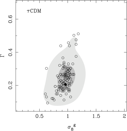
Figure 14: The distribution of best fit parameters in the ($\Gamma,\sigma^{g}_{8}$) plane for mock APM zones taken from the $\tau$CDM Hubble Volume simulation. Each point corresponds to the best fit parameters for the power spectrum recovered from one zone. The darker shaded region encloses the results from $68\%$ of the mocks, the light shading extends this region to enclose $95\%$ of the mocks. The filled circle shows the best fit values of $\Gamma$ and $\sigma^{g}_{8}$ for the galaxy power spectrum measured by FFT in the full simulation box.

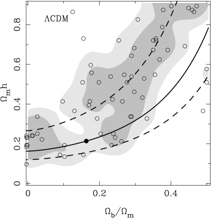
Figure 15: The distribution of best fit parameters in the ($\Omega_{b}/\Omega_{m}$, $\Omega_{m}h$) plane for mock APM zones, this time taken from the $\Lambda$CDM Hubble Volume simulation. Each point corresponds to the best fit parameters for the power spectrum recovered from one mock zone. The heavy shaded region encloses the results from $68\%$ of the mocks, the light shading extends this region to enclose $95\%$ of the mocks. The solid line shows the locus expected in this plane as the baryon fraction is increased for a fixed power spectrum shape, as explained in the text; the dashed lines show the effects of the uncertainty in $\Gamma$. The filled circle shows the best fit values of $\Omega_{b}/\Omega_{m}$ and $\Omega_{m}$ for the galaxy power spectrum measured by FFT in the full simulation box.

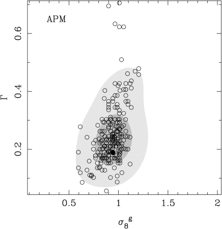
Figure 16: The constraints in the ($\Gamma,\sigma^{g}_{8}$) parameter space from the power spectrum of APM Survey galaxies. The contours show the $68\%$ (heavy) and $95\%$ (heavy plus light) confidence intervals, estimated using mock APM catalogues. The filled circle shows the best fit values of $\Gamma$ and $\sigma^{g}_{8}$ for the galaxy power spectrum measured by FFT in the full simulation box.

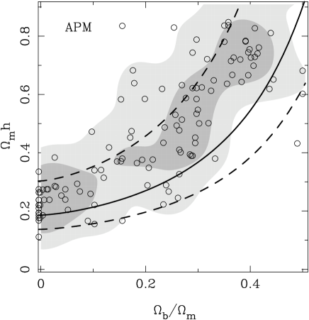
Figure 17: The constraints in the ($\Omega_{b}/\Omega_{m}$, $\Omega_{m}h$) parameter space from the power spectrum of APM Survey galaxies. The contours show the $68\%$ (heavy) and $95\%$ (heavy plus light) confidence intervals, estimated using mock APM catalogues.

We now generalise the comparison presented in the previous section to examine the constraints placed upon the parameters of the CDM model of structure formation by the measurement of the galaxy power spectrum.

In order to simplify the interpretation of the galaxy power spectrum, we restrict our attention to scales on which the underlying density fluctuations are expected to be in the linear regime. We therefore only consider the power spectrum at wavenumbers $k<0.25h$Mpc^-1. The variance in fluctuations in the galaxy distribution when smoothed on this scale is $\sigma=0.1$; Baugh & Efstathiou (1994b) demonstrated that linear perturbation theory still gives an accurate description of the shape of the power spectrum under this condition. A further consequence of focusing on the largest scales is that the relation between fluctuations in the distribution of galaxies and of the dark matter is expected to be a simple scaling in amplitude (e.g. Cole et al. 1998). In this Section, we use the power spectrum of APM Survey galaxies obtained for an evolution of clustering described by $\alpha=1.1$, which we argued is appropriate for the linear regime in the concordance $\Lambda$CDM model (see Section 3).

We consider two sets of parameters that can be used to describe the shape of the power spectrum:

• The amplitude of fluctuations in spheres of radius $8h^{-1}$Mpc, $\sigma^{g}_{8}$, and the power spectrum shape parameter, $\Gamma$, as defined by Efstathiou, Bond & White (1992). Note that we assume $\sigma^{g}_{8}=b\sigma_{8}$, where $b$ is a scale independent bias factor (which applies for $k<0.25h$Mpc^-1).

• The present day mass fraction of baryons, $\Omega_{b}/\Omega_{m}$, and the density parameter times the Hubble constant in units of $100\rm{km}/\rm{s}/\rm{Mpc}$, $\Omega_{m}h$.

Theoretical power spectra are computed for a set of grid points in these parameter spaces using the physically motivated fitting formula given by Eisenstein & Hu (1998); we have checked that this formulation agrees with the output of CMBFAST to better than $10\%$ over the range of wavenumbers considered.

The best pair of parameters that describe a measured power spectrum, $P^{m}$, is found by minimising $\chi^{2}$;

$$\chi^{2}=\sum_{i}(P^{m}(k_{i})-P^{CDM}(k_{i}))^{2}/\sigma_{i}^{2}$$ (13)

where the index $i$ runs over the wavenumber bins $k_{i}$ up to $k=0.25h$Mpc^-1, and $P^{CDM}$ is the theoretical CDM power spectrum. The uncertainty in the measured power spectrum, $\sigma_{i}$, is the rms scatter obtained from the Hubble Volume mocks (see Section 2.7).

The outcome of this procedure is a pair of CDM parameters that best matches the measured $P(k)$. In order to find the variance on the estimate of the best fit parameters, we repeat this process for the power spectra recovered from each mock APM zone. The result is a set of points in the two parameter spaces, either ($\Gamma,\sigma^{g}_{8}$) or ($\Omega_{b}/\Omega_{m}$, $\Omega_{m}h$). The distribution of points is smoothed with a Gaussian filter of width comparable to the spacing of the grid points in each parameter. The smoothed distribution is used to define contours. These contours are then used to delineate regions within which the number of points can be counted to give the $68\%$ and $95\%$ confidence intervals. This process is illustrated in 14, in which we show the constraints in the ($\Gamma,\sigma^{g}_{8}$) plane for the $\tau$CDM mock catalogues. Each point corresponds to the best fit pair of parameters for the power spectrum recovered from a mock APM zone. The dark shading encloses 68% of the points, and the light shading extends this to include 95% of the points. The filled circle shows the best fit values of $\Gamma$ and $\sigma^{g}_{8}$ for the galaxy power spectrum measured by FFT in the full simulation box. The constraints are less strong in the ($\Omega_{b}/\Omega_{m}$, $\Omega_{m}h$) plane, which is plotted in Fig. 17. In this example, we show the results for the $\Lambda$CDM simulation mocks since the initial conditions for the $\Lambda$CDM Hubble Volume simulation were generated using CMBFAST with a baryon fraction of $\Omega_{b}/\Omega_{m}=0.16$, as indicated by the filled circle. The solid curve defines the locus expected in the parameter space to produce a fixed power spectrum shape (for $k<0.25h$Mpc^-1) as the baryon fraction is increased; the dashed lines show how the locus of the parameter space covered in practise due to the uncertainty in $\Gamma$. This curve is a fit to $\Lambda$CDM power spectra generated using the Eisenstein & Hu (1998) formula for the CDM transfer function for an $\Omega_{m}=0.3$ and $\Omega_{\Lambda}=0.7$ cosmology, and can be written as:

$$\Omega_{m}h=\Gamma(1^{+0.6}_{-0.2})\exp\left[5.9(1+1.34^{+0.80}_{-0.33}\Gamma)\left(\frac{\Omega_{b}}{\Omega_{m}}\right)^{1.65+1.23\frac{\Omega_{b}}{\Omega_{m}}}\right].$$

We now apply these parameter constraints to the measured APM Survey power spectrum, using the mock catalogues to define the errors on the parameters. As the mock catalogues were constructed to reproduce an earlier measurement of the power spectrum of APM galaxies, a small rescaling is required in the parameter space, to shift the error contours to lie around the best fitting parameters for our measurement of the power spectrum. The results in the ($\Gamma,\sigma^{g}_{8}$) plane are shown in Fig. 16, with best fit values obtained of $\sigma^{g}_{8}=0.96^{+0.17}_{-0.20}$ and $\Gamma=0.19^{+0.13}_{-0.04}$. Efstathiou & Moody (2001) find similar constraints on these parameters: these authors quote the $2-\sigma$ ranges of $0.78\leq(\sigma^{g}_{8})\leq 1.18$, and $0.05\leq\Gamma\leq 0.38$. Fig. 15 shows the constraints derived from the APM galaxy power spectrum in the ($\Omega_{b}/\Omega_{m}$, $\Omega_{m}h$) plane. Percival et al. (2001) performed a similar analysis using the redshift space power spectrum of 2dFGRS. The shape of the contours in the ($\Omega_{b}/\Omega_{m}$, $\Omega_{m}h$) plane found by Percival et al. are similar to ours, with slightly more curvature for larger values of $\Omega_{m}h$. Percival et al. find somewhat narrower $68\%$ and $95\%$ contours than we do. This is to be expected as a direct estimate of $P(k)$ in three dimensions samples more Fourier modes than is the case for projected data, though the larger volume covered by the APM Survey compared with the 2dFGRS offsets this to some extent.

5 The real space correlation function of APM galaxies

Figure 18: The real space correlation function estimated for APM Survey galaxies using $\alpha=1.7$, divided by a reference power law, with the parameters shown in the legend.

Figure 19: The real space correlation function of APM Survey galaxies. The upper left hand panel compares our estimate of the correlation function (open triangles) with an earlier estimate from Baugh (1996 - filled triangles). The errorbars show the rms scatter from the mocks. We also show, in the same panel, the correlation functions for a SCDM (dashed line) and a $\Lambda$CDM (solid line) models. The lower left panel shows ratios between the APM correlation function estimated in this paper to the SCDM and $\Lambda$CDM correlation functions, using the same line types. The errorbars indicate the amplitude of relative errors as a function of scale $r$. The right hand side panels also show the present estimate of the APM correlation function, but in this case it is compared to the best CDM fits to Boomerang results (Netterfield et al. 2002), for $\sigma_{8}=0.75$ (dashed line) and $\sigma_{8}=0.9$ (solid line). Using the same line styles, the ratios between the APM and CDM correlation functions are shown in the lower right panel.

The two-point galaxy function is still a popular way of characterising galaxy clustering, particularly on small scales. Though it is somewhat less appealing than the power spectrum from a theoretical point of view, the correlation function has the advantage of being simpler conceptually. As the power spectrum and correlation function are Fourier transforms of one another, we can use the measurement of the APM galaxy power spectrum to infer the galaxy correlation function in real space. An independent approach is to write Limber’s equation explicitly in terms of the correlation function, and invert this using the techniques outlined in Section 2 (Baugh 1996). Another possibility is to numerically invert the projected spatial correlation function (Saunders, Rowan-Robinson & Lawrence 1992; Hawkins et al. 2002).

For an isotropic power spectrum, the correlation function is given by:

$$\xi(r)=\frac{1}{2\pi^{2}}\int_{0}^{\infty}P(k)\frac{\sin(kr)}{kr}k^{2}{\rm d}k,$$ (14)

where $r$ is the comoving spatial separation. To avoid spurious numerical artifacts (ringing), the measured power spectrum is extrapolated to high wavenumbers by assuming a suitable power law. We estimate the correlation function from the measured APM power spectrum obtained for both clustering evolution scenarios, $\alpha=1.1$ and $\alpha=1.7$, and give the results in table 2. The relative errors in this table are the rms scatter over the correlation functions obtained from the Fourier transform of the power spectra of the $260$ mock APM zones.

The real space two point correlation function of APM Survey galaxies is well described by a power law, $\xi(r)=(r/r_{0})^{\gamma}$, with $r_{0}=5.9\pm 0.7$ and $\gamma=-1.61\pm 0.06$, as shown in Fig. 18 (here results are shown for the $\alpha=1.7$ case). There is a suggestion that the correlation function rises above a power law for pair separations around $r\sim 10h^{-1}$Mpc and then falls below the power law, as expected in CDM models. However, the size of the errors on our measurement of the correlation function prevents us from making firm statements about these features with any conviction. The correlation function we find is in very good agreement with an independent estimate from the 2dFGRS by Hawkins et al. (2002 - see their Fig. 11). These authors use a different inversion technique to estimate the real space correlation function from the projected correlation function of the 2dFGRS. Hawkins et al. fit a power-law to their estimate of the real space correlation function and obtain a correlation length of $r_{0}=5.05\pm 0.26h^{-1}$Mpc and a slope of $\gamma=-1.67\pm 0.03$.

Figure 19 shows the correlation function for the case where $\alpha=1.7$ (open triangles). In the left-hand panel, we compare this result for $\xi(r)$ with the previous result for the spatial correlation function of APM Survey galaxies, derived by Baugh (1996: filled triangles). The amplitude of our estimate of the correlation function is somewhat higher in amplitude, particularly for $1<r/h^{-1}$Mpc$<10$, as expected from the comparison of the measurements of the power spectrum shown in Fig. 12. Also in the left-hand panel, we compare the measurements of the galaxy correlation function with the theoretical predictions from two flavours of CDM model. The dashed line shows the nonlinear correlation function of the mass in a standard CDM model (SCDM $\Omega_{m}=1$, $\Gamma=0.5$, $\sigma_{8}=0.5$) and the solid line shows the corresponding result for $\Lambda$CDM ($\Omega_{m}=0.3$, $\Omega_{\Lambda}=0.7$, $\Gamma=0.21$, $\sigma_{8}=0.9$). The predictions of the SCDM model lie substantially below the measured galaxy correlation function; the ratio between the measured and theoretical correlation function is shown in the bottom panel. A significant, scale dependent bias factor would be required to reconcile the SCDM model with the measured correlation function. Furthermore, the bias would be required to increase with pair separation, which emphasises that this CDM model has the wrong shape of correlation function. The earlier APM results were used to motivate the need for an anti-bias at small separations, i.e. a reduction in galaxy clustering relative to the dark matter in the $\Lambda$CDM model (Gaztañaga 1995, Jenkins et al. 1998). The comparison with the new correlation function estimate shows that the anti-bias required is much less dramatic than before.

The bottom line on bias changes again if we use a more realistic model for the power spectrum than the simple $\Gamma$ model. The right-hand panel of Fig. 19 compares our measurement of the correlation function with the theoretical predictions for the concordance model used in Section 4.1 (to recap, $\Omega_{m}=0.27$, $\Omega_{\Lambda}=0.67$, $\Omega_{b}=0.05$). These predictions are generated by first producing a linear theory power spectrum with CMBFAST, computing the corresponding nonlinear spectrum using the procedure described by Smith et al. (2002) and finally Fourier transforming the nonlinear mass power spectrum. A normalisation for the amplitude of density fluctuations needs to be specified; we show results for two cases, $\sigma_{8}=0.75$ (dashed line) and $\sigma_{8}=0.9$ (solid line). The lower panel shows that there is no evidence for any anti-bias relative to these models. There is a slight dip in the ratio between the APM and C$\Lambda$CDM correlation functions at a pair separation just below $1h^{-1}$Mpc, which is similar to the feature seen in the correlation function of SDSS galaxies (on a sightly larger scale), as reported by Zehavi et al. 2003. Zehavi et al. interpret this feature as marking the transition between the regime in which correlations between the galaxies in a single halo dominate the clustering signal, to that in which correlations between haloes dominate.

Table 2: The real space correlation function of APM Survey galaxies.

$r/h^{-1}$ Mpc	$\xi(r)$	$\xi(r)$	relative
	$(\alpha=1.1)$	$(\alpha=1.7)$	errors
0.10	578.	615.	0.10
0.13	428.	455.	0.12
0.17	301.	321.	0.084
0.22	210.	223.	0.083
0.28	140.	149.	0.080
0.36	90.9	96.6	0.095
0.47	56.9	60.5	0.095
0.61	35.1	37.4	0.097
0.79	22.6	24.1	0.099
1.03	15.7	16.8	0.11
1.33	10.4	11.1	0.13
1.73	6.54	6.97	0.15
2.24	4.40	4.70	0.16
2.90	2.90	3.09	0.17
3.75	1.99	2.12	0.18
4.86	1.39	1.49	0.21
6.30	0.976	1.04	0.26
8.16	0.674	0.716	0.31
10.6	0.447	0.469	0.36
13.7	0.274	0.282	0.41
17.7	0.150	0.151	0.53
23.0	0.0722	0.0725	0.90
29.8	0.0313	0.0328	1.7
38.6	0.0111	0.0121	2.6
50.0	0.0014	0.0018	7.0

6 Conclusions

We have revised and extended the algorithm introduced by Baugh & Efstathiou (1993) to numerically invert Limber’s equation. A key ingredient of our approach is the use of realistic mock catalogues. These have been used both to test the inversion procedure (extending the work of Gaztañaga & Baugh 1998) and to estimate the errors on the recovered power spectrum or on the value of the parameters of structure formation models. The Lucy inversion technique is competitive with other algorithms described in the literature; it is simple, fast and robust and can be applied over a wide range of scales because it is not underpinned by the assumption of Gaussianity of density fluctuations.

We have also addressed a number of outstanding issues that were raised by the earlier inversion papers. We presented a new model for the redshift distribution of APM Survey galaxies, based upon the latest results from the 2dFGRS (Norberg et al. 2002a). We have also explored the expected evolution of clustering, and put forward arguments to support two particular choices for the value of the parameter $\alpha$ that quantifies the evolution. The assumption that we make about how the power spectrum changes with redshift is undoubtedly an oversimplification, but we have illustrated that the systematic errors incurred through this are typically at most $10\%$ for the case of the APM Survey.

The main impact of the mock catalogues has been in the determination of the errors on our measurement of the power spectrum. The errorbars that we infer are comparable to those inferred by the most recent studies, but can also be obtained at wavenumbers for which Gaussianity is a poor approximation. The errors that we find on the power spectrum on large scales are somewhat larger than those estimated from the scatter between just four measurements by Baugh & Efstathiou (1993, 1994a).

We have used our measurement of the galaxy power spectrum to place constraints upon the main parameters that determine the power spectrum in the CDM model. The constraints we find on the amplitude of fluctuations in the galaxy density, measured in spheres of radius $8h^{-1}$Mpc, $\sigma^{g}_{8}=0.96^{+0.17}_{-0.20}$ and on the shape of the power spectrum, $\Gamma=0.19^{+0.13}_{-0.04}$, are comparable to previous results obtained for the APM Survey by Efstathiou & Moody (2001). Dodelson et al. (2002) inverted the angular clustering in an early data release of the SDSS and found $\Gamma=0.14^{+0.11}_{-0.06}$, in agreement with our constraint. Szalay et al. (2001) used a KL estimate of the power spectrum from the SDSS to derive a similar range of values: $\Gamma=0.188\pm 0.04$ and $\sigma^{g}_{8}=0.915\pm 0.06$ for a flat universe with cosmological constant. A consensus seems to be emerging on the shape and amplitude of the galaxy power spectrum for bright, optically selected galaxies, as remarked upon by Hoyle et al. (1999).

The galaxy power spectrum that we measure is in good agreement with the shape of the linear perturbation theory power spectrum of the “concordance” $\Lambda$CDM model on large scales. On small scales, the form of the galaxy power spectrum is strongly discrepant with the linear theory mass spectrum. A large part of this disagreement is accounted for when the nonlinear evolution of the density field is taken into consideration. The remaining differences between the galaxy power spectrum and the nonlinear power spectrum of the mass are at present being studied with the aid of hierarchical models of galaxy formation. It will be of particular interest to study how the relationship between the distribution of galaxies and the underlying mass evolves with redshift by applying the technique set out in this paper to narrow redshift slices of galaxies selected using photometric redshifts from forthcoming, deep, multi-passband surveys.

References

- [] Allgood, B., Blumenthal,G. & Primack,J.R., 2001, conference proceeding for ”Where’s the Matter”, Marseille.
- [] Baugh, C.M., 1996, MNRAS, 280, 267.
- [] Baugh, C.M. & Efstathiou, G., 1993, MNRAS, 265, 145.
- [] Baugh, C.M. & Efstathiou, G., 1994a, MNRAS, 267, 323.
- [] Baugh, C.M. & Efstathiou, G., 1994b, MNRAS, 270, 183.
- [] Baugh, C.M., Gaztañaga, E. & Efstathiou, G., 1995, MNRAS, 274, 1049.
- [] Baugh, C.M., Benson, A.J., Cole,S., Frenk, C.S., Lacey, C.G., 1999, MNRAS, 305, L21.
- [] Benson, A.J., Cole, S., Frenk, C.S., Baugh, C.M., Lacey, C.G., 2000, MNRAS, 311, 793.
- [] Cole, S., Hatton, S., Weinberg, D. H. & Frenk, C. S., 1998, MNRAS, 300, 945.
- [] Colless, M. et al. (the 2dFGRS Team), 2001, MNRAS, 328, 1039.
- [] Connolly, A. et al. (the SDSS Collaboration), 2002, ApJ, 579, 42.
- [] Croft, R.A.C., Weinberg, D.H., Pettini, M., Hernquist, L., Katz, N., 1999, ApJ, 520, 1.
- [] Croft, R.A.C., Weinberg, D.H., Bolte, M., Burles, S., Hernquist, L., Katz, N., Kirkman, D. & Tytler, D., 2002, ApJ, 581, 20.
- [] de Bernardis, P. et al., 2000, Nature, 404, 955.
- [] Dodelson, S. & Gaztañaga, E., 2000, MNRAS, 312, 774.
- [] Dodelson, S. et al. (the SDSS Collaboration), 2002, ApJ, 572, 140.
- [] Efstathiou, G., Sutherland, W. J. & Maddox, S. J., 1990, Nature, 348, 705.
- [] Efstathiou, G., Bond, J.R. & White, S.D.M., 1992, MNRAS, 258, 1P.
- [] Efstathiou, G. & Moody, S.J., 2001, MNRAS, 325, 1603.
- [] Efstathiou, G. et al. (the 2dFGRS Team), 2002, MNRAS, 330, L29.
- [] Eisenstein, D.J. & Hu, W., 1998, ApJ, 496, 605.
- [] Eisenstein, D.J. & Zaldarriaga, M., 2001, ApJ, 546, 2.
- [] Eke, V.R., Cole, S. & Frenk, C.S., 1996, MNRAS, 282, 263.
- [] Evrard, A.E. et al. (the Virgo Consortium), 2002, ApJ, 573, 7.
- [] Gaztañaga, E., 1995, ApJ, 454, 561.
- [] Gaztañaga, E. & Baugh, C.M., 1998, MNRAS, 294, 229.
- [] Gnedin, N.Y. & Hamilton, A.J.S., 2002, MNRAS, 334, 107.
- [] Hamilton, A.J.S. & Tegmark, M., 2002, MNRAS, 330, 506.
- [] Hawkins, E. et al. (the 2dFGRS Team), 2002, astro-ph/0212375.
- [] Hoyle,F., Baugh, C.M., Shanks, T. & Ratcliffe, A., 1999, MNRAS, 309, 659.
- [] Jaffe, A. H., et al. 2001, PhRvL, 86, 3475.
- [] Jarrett, T.H., Chester, T., Cutri, R., Schneider, S., Skrutskie, M., Huchra, J.P., 2000, AJ, 119, 2498.
- [] Jenkins, A. et al. (the Virgo Consortium), 1998, ApJ, 499, 20.
- [] Limber, D.N., 1954, ApJ, 119, 655.
- [] Lucy, L.B., 1974, AJ, 79, 745.
- [] Lucy, L.B., 1994, A&A, 289, 983.
- [] Maddox, S.J., Efstathiou, G., Sutherland, W.J., Loveday,J., 1990, MNRAS, 243, 692.
- [] Maddox, S.J., Efstathiou, G., Sutherland, W.J., 1996, MNRAS, 283, 1227.
- [] Maller, A.H., McIntosh, D.H., Katz, N., & Weinberg, M.D., 2003, submitted to ApJ, Astro-ph/0304005.
- [] McCracken, H.J., Le Fèbre, O., Brodwin, M., Foucaud, S., Lilly, S.J., Crampton, D., Mellier, Y., 2001, A&A, 376, 756.
- [] Meiksin, A. & White, M., 1999, MNRAS, 308, 1179.
- [] Netterfield, C.B., et al., 2002, ApJ, 571, 604.
- [] Norberg, P. et al. (the 2dFGRS Team), 2001, MNRAS, 328,64.
- [] Norberg, P. et al. (the 2dFGRS Team), 2002b, MNRAS, 332, 827.
- [] Norberg, P. et al. (the 2dFGRS Team), 2002a, MNRAS, 336, 907.
- [] Ostriker, J.P., Steinhardt, P.J., 1995, Nature, 377, 600.
- [] Padilla, N.D., & Baugh, C.M., 2002, MNRAS, 329, 431.
- [] Peacock, J.A., 1991, MNRAS, 253, 1.
- [] Peacock, J. A., 1997, MNRAS, 284, 885.
- [] Peacock, J.A. & Dodds, S.J., 1996, MNRAS, 280, 19.
- [] Peebles, P.J.E., 1980, The Large-Scale Structure of the Universe. Princeton Univ. Press, Princeton.
- [] Peebles, P.J.E., 1993, Principles of Physical Cosmology. Princeton Univ. Press, Princeton.
- [] Percival, W.J. et al. (the 2dFGRS Team), 2001, MNRAS, 327, 1297.
- [] Percival, W.J. et al. (the 2dFGRS Team), 2002, MNRAS, 337, 1068.
- [] Perlmutter, S. et al., 1999, ApJ, 517, 565.
- [] Saunders, W., Rowan-Robinson, M., Lawrence, A., 1992, MNRAS, 258, 134.
- [] Saunders, W. et al., 2000, MNRAS, 317, 55.
- [] Scoccimarro, R., Sheth, R.K., 2002, MNRAS, 329, 629.
- [] Seljak, U., Zaldarriaga, M., 1996, ApJ, 469, 437.
- [] Smith, R.E. et al. (the Virgo Consortium), 2002, astro-ph/0207664.
- [] Sutherland, W. et al., 1999, MNRAS, 308, 289.
- [] Szalay, A. et al. 2001, astro-ph/0107419.
- [] Tadros, H. & Efstathiou, G., 1996, MNRAS, 282, 1381.
- [] Zaldarriaga, M., Scoccimarro, R. & Hui, L., 2001, astro-ph/0111230.
- [] Zehavi et al., 2003, submitted to ApJ, astro-ph/0301280.
- [] Zucca, E. et al., 1997, A&A, 326, 477.