Determining Foreground Contamination in CMB Observations:
Diffuse Galactic Emission in the MAXIMA-I Field

Abstract

Observations of the CMB can be contaminated by diffuse foreground emission from sources such as Galactic dust and synchrotron radiation. In these cases, the morphology of the contaminating source is known from observations at different frequencies, but not its amplitude at the frequency of interest for the CMB. We develop a technique for accounting for the effects of such emission in this case, and for simultaneously estimating the foreground amplitude in the CMB observations. We apply the technique to CMB data from the MAXIMA-1 experiment, using maps of Galactic dust emission from combinations of IRAS and DIRBE observations, as well as compilations of Galactic synchrotron emission observations. The spectrum of the dust emission over the 150–450 GHz observed by MAXIMA is consistent with preferred models but the effect on CMB power spectrum observations is negligible.

1 Introduction

Measurements of the Cosmic Microwave Background (CMB) have begun to fulfill their promise to image the Universe at the epoch of the decoupling of photons from baryons, thereby measuring cosmological parameters to new levels of precision. In recent years, the balloon-borne bolometer experiments MAXIMA-1 (Hanany et al., 2000; Lee et al., 2001; Rabii et al., 2003), BOOMERANG (de Bernardis et al., 2000; Netterfield et al., 2002) and Archeops (Benoit et al., 2002), as well as the ground-based interferometers, CBI (Padin et al., 2001; Mason et al., 2002), DASI (Halverson et al., 2002) and VSA (Grainge et al., 2002) have measured the CMB power spectrum down to angular scales of 10 arcminutes or better; most recently, WMAP has observed the full CMB sky over a factor of four in frequency and with a beam of 13 arcmin FWHM. The CMB photons are produced at the last scattering surface, when the opaque, charged plasma of electrons and nuclei becomes a transparent gas of hydrogen and helium, at a temperature of about 1 eV, the epoch of “Recombination.” The measured signals thus map the primordial distribution of matter in the Universe, and allow measurements of the cosmological parameters and an understanding of the mechanism for laying down the initial fluctuations.

This promise has, however, always been tempered by the possibility of contamination from astrophysical sources of microwave emission or absorption, even away from the Galactic plane. Happily, the cosmological signal has proven to be dominant over a wide range of frequencies and angular scales. Nonetheless, we can hope to isolate these foreground contributions: the CMB itself has the well-understood shape of a black-body spectrum at a given temperature. Other contributions, Galactic or extragalactic, will in all but the most pathological cases have a different spectral dependence. While the peak of the 2.73K CMB intensity lies at about 90 GHz, other contributions dominate at other frequencies (e.g., Tegmark et al., 2000). Emission from dust (and dusty external galaxies) is expected to dominate the CMB at higher frequencies; synchrotron and free-free emission (and galaxies radiating by these methods) dominate at lower frequencies.

Very often, then, we will have independent measurements of the contribution from a given foreground component. However, because those measurements are taken at a different frequency than those of the CMB measurements, we must extrapolate down to the frequencies of interest. As we inevitably lack a perfect understanding of the foreground emission mechanism, this extrapolation will be imprecise.

In this work, we present a framework for dealing with such imprecise extrapolation, by leaving the spectral dependence free to vary, but fixing the morphology to be determined by the external measurements. The method allows us, on the one hand, to determine the global spectral behavior of the foreground component and “marginalize over” (in Bayesian parlance) the CMB signal, or, on the other hand, to determine the CMB signal while marginalizing over the foreground contribution. Similar methods have been proposed in the past with more ad hoc derivations (e.g., Dodelson & Stebbins, 1994; Tegmark & Efstathiou, 1996; Dodelson, 1997; Tegmark, 1998; de Oliveira-Costa & Tegmark, 1999, and references therein). Here, we show how the same formalism can deal with several different foreground problems: estimating the amplitude of the foreground emission; estimating the CMB map after accounting for the foregrounds; and finally estimating the CMB power spectrum in the presence of such contamination.

In this paper we concentrate on the contribution of Galactic dust emission to the emission observed by the MAXIMA-1 experiment at 150–410 GHz. As our foreground template, we use the recent seminal work of Finkbeiner et al. (1999), who combined data from the IRAS satellite with that from the DIRBE and FIRAS instruments on the COBE satellite to extrapolate the spectrum of Galactic dust pixel-by-pixel to our CMB frequencies. These maps were also used in the analysis of the dust signal present in BOOMERANG data (Masi et al., 2001).

Finally, we note that the recent work of the WMAP team takes a somewhat different approach, using a maximum-entropy method to estimate foreground emission (Bennett et al., 2003). In that work, they too use the Finkbeiner et al. (1999) maps as a “prior” for the dust emission. However, the effective sensitivity of the WMAP dust reconstruction is comparable to the CMB sensitivity. Thus, in regions of very low dust contrast such as that observed by MAXIMA-1, the WMAP prediction of dust emission is insufficiently sensitive, and indeed imperfectly correlated with the input prior maps.

2 Methods

In this paper, we are concerned with the possible contribution from the aforementioned sources of Galactic foreground emission, in particular contamination by dust emission. We will further assume that we have a robust measurement of the foreground at some frequency other than that with which we observe the CMB. For example, dust is dominant at high frequencies, $f\gtrsim 300$ GHz, but believed to be only a small contaminant at the 50–200 GHz at which the CMB dominates high-Galactic latitude emission.

Thus, we will assume that the spatial pattern of these sources is known, and described by some template, $f_{ip}$, where $p$ numbers the observed pixels in our CMB maps, and $i$ labels the various foreground contributions (e.g., dust, synchrotron, etc.). However, we will leave the amplitude of the individual foreground contributions to be determined. That is, $f_{ip}$ is the foreground map, at its observed frequency for example. This will be multiplied by an unknown amplitude $\beta_{i}$, to be determined as the result of our analysis.

For the purposes of this paper, then, the intensity in a pixel of our CMB map is given by

$$d_{p}=\sum_{i}\beta_{i}f_{ip}+s_{p}+n_{p}$$ (1)

where $d_{p}$ is the data at pixel $p$; $s_{p}$ is the CMB signal at that pixel; $n_{p}$ is the noise in the pixel; and $\sum_{i}\beta_{i}f_{ip}$ gives the total contribution from the foreground sources under consideration. We take the CMB signal and the foreground template to be already smeared by the beam and any other instrumental effects:

$$s_{p} = \int d^{2}{\bf\hat{x}}\;B({\bf\hat{x}},{\bf\hat{x}}_{p})T({\bf\hat{x}})$$ (2)

$$= \int d^{2}{\bf\hat{x}}\;B({\bf\hat{x}}\cdot{\bf\hat{x}}_{p})T({\bf\hat{x}})$$

$$= \sum_{\ell m}B_{\ell}a_{\ell m}Y_{\ell m}({\bf\hat{x}}_{p})\;,$$

where $B({\bf\hat{x}},{\bf\hat{x}}_{p})$ gives the response of the beam at position ${\bf\hat{x}}$ when pointed at pixel $p$. In the second equality we assume that the beam is azimuthally symmetric around pixel $p$, and in the third equality we transform to spherical harmonics with indices $(\ell,m)$. Here, $B_{\ell}$ is the transform of the symmetric $B({\bf\hat{x}}\cdot{\bf\hat{x}}_{p})$ and $a_{\ell m}$ is the transform of $T({\bf\hat{x}})$. For more information on working with asymmetric beams and pixels, see Wu et al. (2001); Souradeep & Ratra (2001).

Note that this model, Eq. 1, is essentially the same as that considered in Stompor et al. (2002), although that work considers a broader class of templates, $f_{ip}$, allowing them to be associated with an amplitude synchronous with instrumental characteristics rather than the sky. That work then derives techniques, analogous to the ones described below, to determine or marginalize over these amplitudes.

Under this model, we can ask two separate questions:

1. What are the foreground amplitudes, $\beta_{i}$?

2. What is the underlying signal, $s_{p}$? Perhaps more important is the related question: What is $C_{\ell}$? That is, what are the statistics of the cosmological component, $s_{p}$, taking into account the possible presence of foreground contamination?

To answer these questions we must first assign appropriate distributions to the quantities in Eq. 1. As usual, the noise is taken to be distributed as a zero-mean Gaussian with covariance $N_{pp^{\prime}}\equiv\langle n_{p}n_{p^{\prime}}\rangle$ (assumed known beforehand, although we can also apply iterative techniques (Ferreira & Jaffe, 2000; Doré et al., 2001) to determine it simultaneously with the CMB and foreground signals). This gives a likelihood function

$$P(d|\beta,s) = \frac{1}{\left|2\pi N\right|^{1/2}}\times$$ (3)

$$\exp\left[{-\frac{1}{2}(d-s-\beta f)^{T}N^{-1}(d-s-\beta f)}\right]\;,$$

where we have left off indices and used matrix notation.

In order to determine the underlying signal power spectrum, we will need to assign an appropriate Gaussian distribution, with variance given by

$$S_{pp^{\prime}}\equiv\langle s_{p}s_{p^{\prime}}\rangle=\sum_{\ell}\frac{2\ell+1}{4\pi}B^{2}_{\ell}C_{\ell}P_{\ell}(\cos\theta_{pp^{\prime}}),$$ (4)

where $C_{\ell}\equiv\langle|a_{\ell m}|^{2}\rangle$ is the underlying CMB power spectrum, $\theta_{pp^{\prime}}$ is the angle between pixels $p$ and $p^{\prime}$, and the $P_{\ell}$ are the Legendre polynomials. This gives a distribution

$$P(s|C_{\ell})=\frac{1}{\left|2\pi N\right|^{1/2}}\exp\left[-\frac{1}{2}s^{T}S^{-1}s\right]\;.$$ (5)

All of this is as in the usual foreground-free case. The likelihood for the data $d$ (given $\beta$ and $s$) is a Gaussian, now with mean $\sum_{i}\beta_{i}f_{ip}+s_{p}$. Finally, however, we must assign a prior to the amplitudes $\beta_{i}$. To remain sufficiently general, we will allow an arbitrary Gaussian for each amplitude, with $\langle\beta_{i}\rangle=0$, and $\langle\beta^{2}\rangle=\sigma_{\beta i}^{2}$. The prior is then

$$P(\beta)=\prod_{i}\frac{1}{\sqrt{2\pi\sigma_{i}^{2}}}\exp\left[-\frac{1}{2}\frac{\beta_{i}^{2}}{\sigma_{\beta i}^{2}}\right]\;.$$ (6)

We can take $\sigma_{\beta i}\to\infty$ to give a ‘non-informative’ distribution. This is algebraically easier to deal with than the equivalent unbounded uniform distribution.

If we combine these priors with the likelihood, we use Bayes’ theorem to get the posterior distribution

$$P(\beta_{i},s_{p}|C_{\ell},d_{p})\propto P(\beta_{i})P(s_{p}|C_{\ell})P(d_{p}|\beta_{i},s_{p},C_{\ell})$$ (7)

where $P(\beta_{i})$ and $P(s_{p}|C_{\ell})$ are priors, and $P(d_{p}|\beta_{i},s_{p})$ is the likelihood. Then, in order to answer each of the above questions, we marginalize over $\beta$ to get the posterior for $s$; $s$ to get the posterior for $\beta$; and finally marginalize over both, after giving $s$ the appropriate prior variance appropriate for a given $C_{\ell}$. Because of the linear, Gaussian form of our likelihood and priors, all of these marginalizations essentially involve “completing the square,” and each of the posteriors remains a Gaussian distribution. For the same reason, these results can also be derived on the usual minimum-variance grounds rather than in this Bayesian formalism.

First, we calculate the posterior distribution of $\beta$ by marginalizing over $s_{p}$:

$$P(\beta|d_{p},C_{\ell}) = \int ds\;P(\beta,s|d,C_{\ell})$$ (8)

$$= \frac{1}{|2\pi M_{\beta}|^{1/2}}\times$$

$$\exp\left[-\frac{1}{2}(\beta-{\bar{\beta}})^{T}M_{\beta}^{-1}(\beta-{\bar{\beta}})\right]$$

This is a Gaussian with mean

$${\bar{\beta}}_{i}=\langle\beta_{i}\rangle=\left[f^{T}(S+N)^{-1}f\right]_{ii^{\prime}}^{-1}(f^{T}(S+N)^{-1}d)_{i^{\prime}}$$ (9)

and covariance

$$M_{\beta,ii^{\prime}}=\langle(\beta-{\bar{\beta}}_{i})(\beta-{\bar{\beta}}_{i^{\prime}})\rangle=\left[f^{T}(S+N)^{-1}f\right]_{ii^{\prime}}^{-1}\;.$$ (10)

We have already taken the prior variances $\sigma_{\beta i}\to\infty$ in this expression. As is often the case in linear problems with normal errors as we have here, this is just the least squares solution for the amplitudes, $\beta_{i}$.

The posterior for the signal, $s_{p}$, is also a Gaussian. It has mean

$${\bar{s}}_{p}=S(S+N+\sigma_{\beta}^{2}ff^{T})^{-1}d$$ (11)

and covariance

$$\langle(s-{\bar{s}}_{p})(s-{\bar{s}}_{p^{\prime}})\rangle = S(S+N+\sigma_{\beta}^{2}ff^{T})^{-1}(N+\sigma_{\beta}^{2}ff^{T})$$ (12)

$$= S-S(S+N+\sigma_{\beta}^{2}ff^{T})^{-1}S\;.$$

This gives us the Wiener Filter as the mean of this distribution. Note that we have left in a finite prior variance for $\beta_{i}$. We can take these prior variances to infinity using the Sherman-Morrison-Woodbury formula, which states

$$(W+fBf^{T})^{-1}=W^{-1}-W^{-1}f(f^{T}W^{-1}f-B^{-1})^{-1}f^{T}W^{-1}\;.$$ (13)

Setting $W=S+N$ and $B^{-1}=\sigma_{\beta}^{-2}I\to 0$ here is equivalent to marginalizing over our template amplitudes. Note that, as in Stompor et al. (2002), this same formula can be applied in the determination of the original map, $d_{p}$, in order to marginalize over such modes at an earlier stage.

Finally, we wish to determine the power spectrum, $C_{\ell}$. We do this by starting with the expression in Eq. 7, and using Bayes’ theorem yet again:

$$P(C_{\ell}|d_{p})\propto P(C_{\ell})P(d_{p}|C_{\ell})=P(C_{\ell})\int d\beta\;dsP(\beta,s|d,C_{\ell})\;.$$ (14)

(Equivalently, we could have considered $C_{\ell}$ a “parameter” from the start, and just given it a delta function prior when calculating the distributions of $\beta$ and $s$.) In this case, it is worth writing out the entire expression:

$$P(C_{\ell}|d)=P(C_{\ell})\frac{1}{\left|2\pi M\right|^{1/2}}\exp\left[-\frac{1}{2}d^{T}M^{-1}d\right]$$ (15)

where the covariance matrix is given by

$$M_{pp^{\prime}} = \langle d_{p}d_{p^{\prime}}\rangle=\sum_{ii^{\prime}}f_{ip}\langle\beta_{i}\beta_{i^{\prime}}\rangle f_{i^{\prime}p^{\prime}}+\langle s_{p}s_{p^{\prime}}\rangle+\langle n_{p}n_{p^{\prime}}\rangle$$ (16)

$$= (\sigma_{\beta}^{2}f^{T}f)_{pp^{\prime}}+S_{pp^{\prime}}+N_{pp^{\prime}}\;.$$

Recall that the signal covariance is a function of the underlying power spectrum, $C_{\ell}$, as in Eq. 4. We then maximize this with respect to the $C_{\ell}$ (or bands thereof with known shape) as in Bond et al. (1998) as implemented in MADCAP (Borrill, 1999). In this expression, we have kept a finite variance for the dust prior, $\sigma^{2}_{\beta}$. In the absence of a known dust contaminant spectrum (or to be most conservative), we can take $\sigma_{\beta}\to\infty$. The numerical implementation of this can be done using the Sherman-Morrison-Woodbury formula, implemented in the current version of MADCAP.

Note that it is the linear nature of our model Eq. 1, along with our assignment of Gaussian priors and likelihoods, that allows these analytic simplifications. This makes it somewhat more difficult to determine or marginalize over more physical parameters such as, say, the spectral index of the foreground spectra. However, we can use this formalism to determine several $\beta_{i}$, each corresponding to a different region of the sky — allowing us to take account at some level of spatial variations in the spectrum. For the present case, however, the final signal-to-noise is too low for this to be fruitful.

In the Bayesian picture, our method simply ignores any information associated with a pattern on the sky matching our chosen templates. Thus, even if our template were “wrong” (i.e., if they did not accurately reflect the pattern of foreground emission on the sky), the final estimate of the power spectrum, including its error bars, would be no less correct than that without applying this method at all. In the simplest case, the maximum likelihood power could decrease, but the error bars would increase to take this into account.

2.1 Noisy Foreground Templates

So far, we have only considered foreground templates, $f$, that are accurately known. In many cases, however, the pattern will also be the result of a noisy measurement. That is, we supplement our model of the data, Eq. 1 with a new set of pixel measurements,

$$e_{p}=f_{p}+\nu_{p}$$ (17)

where $e_{p}$ is the new data, $\nu_{p}$ is noise, satisfying $\langle\nu_{p}\nu_{p^{\prime}}\rangle=E_{pp^{\prime}}$, and we can again assign a Gaussian error distribution for $\nu_{p}$. Now, to proceed we must multiply this new distribution by the likelihood of Eq. 3 or the full Eq. 7, and marginalize over the now unknown template, $f$:

$$P(de|\beta,s) = \frac{1}{\left|2\pi N+\beta^{2}E\right|^{1/2}}\times$$ (18)

$$\exp\left[{-\frac{1}{2}(d-s-\beta e)^{T}(N+\beta^{2}E)^{-1}(d-s-\beta e)}\right]\;.$$

After marginalization, the variance is increased by $\beta^{2}E$ over the case where the foreground template is known exactly. As before, we can also put in a prior for the signal amplitude, $s$ (Eq. 5), and marginalize, giving the equivalent of Eq. 15,

$$P(C_{\ell}|de)=P(C_{\ell})\frac{1}{\left|2\pi(S+N+\beta^{2}E)\right|^{1/2}}\exp\left[-\frac{1}{2}(d-\beta e)^{T}(S+N+\beta^{2}E)^{-1}(d-\beta e)\right]\;.$$ (19)

In both cases, the marginalization over the foreground template has destroyed the linear nature of the problem, and the unknown amplitude, $\beta$ now appears in the effective correlation matrix; we can no longer find analytic formulae to determine nor marginalize over the amplitude

In fact, the problem for a noisy template is formally identical to the cross-calibration of cross-comparison problem, as discussed in Knox et al. (1998): the amplitude, $\beta$ is just the relative calibration of the foreground contribution to the two datasets. As in that work, however, we must use somewhat more laborious numerical techniques to deal with the more complicated problem.

3 Application: Diffuse foregrounds and MAXIMA-1

Here we apply these techniques to the data from the MAXIMA-I experiment; the hardware is described in Lee et al. (1999) the resulting maps and power spectra are described in Hanany et al. (2000); Lee et al. (2001), the cosmological implications are presented in Balbi et al. (2000); Stompor et al. (2001); Jaffe et al. (2001) and details of the data analysis in Stompor et al. (2002). In this work, we consider maps made from the data of individual photometers at various frequencies: three at 150 GHz, two at 240 GHz, and two at 410 GHz. Note that only a subset of these maps were used for the cosmological results presented in the previous MAXIMA-I papers. A full account of the systematic checks on the MAXIMA-I data and on the consistency between channels is given in Stompor et al. (2003).

The primary aim of the MAXIMA experiment is to observe the cosmological component of the CMB. The MAXIMA-I field was thus explicitly chosen to be low in Galactic foreground emission. Nonetheless, our methods let us take advantage of the large number of pixels simultaneously, even though the dust contribution is insignificant in a single one.

3.1 Dust Emission from Galactic Cirrus

As foreground templates, we primarily work with the combined IRAS/DIRBE infrared dust maps presented in Schlegel et al. (1998). These are extrapolated from 100-240µm to our CMB observation frequencies using dust emissivity models constrained by COBE/FIRAS spectral observations (Finkbeiner et al., 1999). One can use these emissivity models to compute a dust temperature and column density in each pixel from the DIRBE 100 and 240µm maps, and extrapolate to much lower frequencies. Although our formalism could be used to extrapolate from the observed infrared frequencies down to our observations at 100-400 GHz, neglect of the dust temperature variation from pixel to pixel can cause errors of a factor of $\sim 2$, so we use the FDS99 models that already take account of this variation explicitly. Eight models are computed; four single-model components (power laws) and four two-component models (where the two components have a fixed mass ratio, and have temperature coupled to the radiation field in a self-consistent way). The parameters of the model are given in Table 1, adapted from FDS99. The 4 parameters describing each model are: $\alpha_{1},\alpha_{2}$, the emissivity power-law indices for components one and two, $f_{1}$, the fraction of power absorbed and re-emitted by component 1 (unrelated to the foreground template vector $f$ above), and $q_{1}/q_{2}$ where $q_{i}$ is the IR/optical opacity ratio for component $i$. The two-component models listed in the table are: 5) $T_{1}=T_{2}$, indices from Pollack et al. (1994), 6) $\alpha_{1}=\alpha_{2}=2$ as in Reach et al. (1995), 7) like 5 except temperatures can float, and 8) all four parameters floating. Because 8 gives the best chi-squared, it is the preferred model, although 7) is not appreciably different. Here, we will concentrate on their overall best-fit model 8, with $\alpha_{1}=1.67$, $\alpha_{2}=2.70$, $f_{1}=0.0363$, and $q_{1}/q_{2}=13.0$.

In Figures 1, 2, and 3 we show the MAXIMA-1 data as well as the SFD extrapolated dust maps (using their preferred Model 8) at each of these frequencies. Note that the temperature scale for the dust at 150 and 240 GHz is stretched considerably compared to the data – the expected RMS dust contribution is $\sim 1\mu$K at 150 GHz, compared to the $\sim 300\mu$K (signal plus noise) RMS of the 150 GHz CMB map.

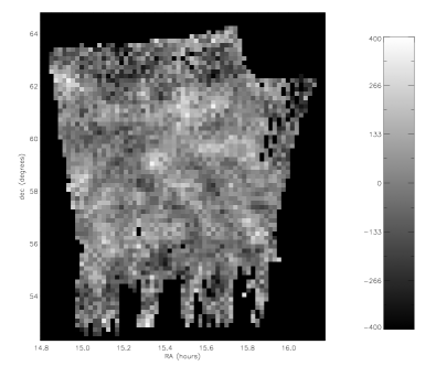
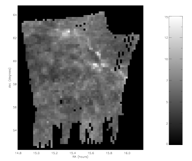
Figure 1: Left: MAXIMA-I map of microwave emission at 150 Ghz. Right: Map of dust emission, extrapolated from IRAS/DIRBE maps to 150 GHz. Colorbars give the temperature in $\mu$K. Note that the difference in the temperature range between the total and dust emission is a factor of $\sim 50$.

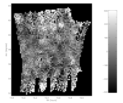
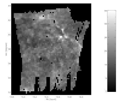
Figure 2: Left: MAXIMA-I map of CMB Emission at 240 Ghz. Right: Map of dust emission, extrapolated from IRAS/DIRBE maps to 240 GHz. Note that the difference in the temperature range between the total and dust emission is a factor of $\sim 17$.

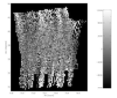
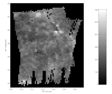
Figure 3: Left: MAXIMA-I map of CMB Emission at 410 Ghz. Right: Map of dust emission, extrapolated from IRAS/DIRBE maps to 410 GHz. Note that the difference in the temperature range between the total and dust emission is a factor of $\sim 40$.

Because of this large difference in the amplitude of CMB and dust emission, we do not expect to be able to see the dust contribution to a single pixel in the maps. However, our procedure for estimating $\beta$ gives us the usual $(N_{\rm DOF})^{1/2}$ advantage when considering the whole map ($N_{\rm DOF}$ gives the number of degrees of freedom in the map, equal to the number of pixels less any degrees of freedom marginalized over in making the map or by the methods described here). We can further increase the signal-to-noise by combining the individual photometers at a given frequency. This allows us to compare the different models offered by SFD, as detailed in their work.

In Figure 4, we show the observed amplitude $\beta$ for each SFD model, for the MAXIMA-I detectors combined at each of 150, 240 and 410 GHz, and combined over all frequencies (the latter makes sense only if the overall spectral shape of the model is correct over this frequency range). The data do not strongly prefer any single model. However, a few results are evident.

Figure 4: Each panel gives the observed amplitude of the dust template for the model number given on the horizontal axis at a given frequency. The top panel averages over all frequencies.

The dust signal is not strongly detected at 150 or 410 GHz for any model. That is, at these frequencies an amplitude of $\beta=0$ is not disfavored. Indeed, some of the models are disfavored at roughly the one sigma level from the 240 GHz data, with the one-component model 1 the most disfavored. At 410 GHz, the dust signal is stronger, and $\beta=1$ (the model prediction) is preferred over $\beta=0$ in all cases.

Despite the only marginal preference for a non-zero signal, these results do contain important information. Even in the cases where $\beta=0$ is allowed, the results can be interpreted as an upper limit on the dust amplitude at these frequencies and in this area of sky. As is evident from equations 9 and 10, the observed amplitude and error scale inversely with the template amplitude. Thus, although $\beta=1$ is acceptable for all of these models, models predicting dust emission a factor of a few higher at any of these frequencies would be strongly disfavored.

In Figure 5, we show the results for SFD’s Model 8 — their overall best fit — in detail. We show each of the individual detector amplitudes, the frequency averages, as well as an overall average. In Figure 6, we rescale the observed coefficients $\beta$ to give the actual values of the observed dust emission amplitude in thermodynamic temperature units.

Figure 5: Ratio of expected amplitude of dust emission (SFD Model 8) to that observed in the MAXIMA-I maps, as a function of detector frequency (offset slightly for legibility). Thin error bars with circles are individual detectors, thick error bars with crosses at the individual frequencies (150, 240, 410) combine these, and the single error bar at $f\sim 300$ gives the overall average.

Figure 6: Thermodynamic temperature of dust emission observed in each of the three MAXIMA-I frequencies. The curve gives the average emission from Finkbeiner et al’s Model 8 predicted in the MAXIMA-I observation area.

This figure emphasizes that the techniques described here are not only useful for the removal of CMB foregrounds, but are more generally useful for estimating the foreground spectrum and extrapolating it to regimes where it may be completely negligible in an individual pixel.

3.2 Synchrotron Emission

We can of course use the same algorithm with other sources of foreground emission for which we have maps. The FSD code also provides an extrapolation synchrotron emission as measured by Haslam et al. (1981); Reich & Reich (1986); Jonas et al. (1998).

These surveys were reprocessed, destriped, and point-source subtracted (D.P. Finkbeiner 2002, private communication) and are available to the public as part of the dust map distribution.

The Haslam survey is full-sky, the Reich & Reich survey is in the north, and the Rhodes survey in the south, so for every point on the sky at least two frequencies are available. The surveys are beam-matched (at a one degree resolution) and used to determine a power law for each pixel on the sky. This power law is then extrapolated to the frequency of observation. Because the synchrotron spectrum is known to fall faster than a power law at high frequencies, this prediction should be interpreted as an upper limit on the synchrotron emission. If the 408 – 2326 MHz maps are contaminated by significant free-free emission, the power law slope is shallower than it should be, making it even more of an upper limit. The fact that even this upper limit is smaller than $3\mu$K at 150 GHz over the MAXIMA area implies that the synchrotron emission should be totally undetectable. Figure 7 confirms this to the extent possible with this data.

Figure 7: Observed synchrotron emission relative to that expected, as in figure 5.

3.3 The CMB power spectrum

Now that we have measured the overall level of dust emission in the MAXIMA-I field, we can now ask the other questions posed in Section 2: what does the CMB itself look like? In figure 8, we show the power spectrum of CMB temperature fluctuations from the combined 150 GHz photometers (as used in Lee et al. (2001) and Stompor et al. (2001)). One set of points shows the spectrum ignoring the contamination from dust and synchrotron emission ($\sigma_{\beta}\to 0$ in equations 15 and 16); the other set marginalizes over the dust emission with the known morphology of FSD’s model 8 ($\sigma_{\beta}\to\infty)$. We see that the marginalization has very little effect — much smaller than the error bars. This is consistent with our knowledge of the power spectrum of high-latitude dust emission, with $C_{\ell}\sim\ell^{-3}$ (or perhaps closer to $\ell^{-2}$ in some parts of the sky), dominating only at the largest scales. This implies that the spatial pattern of the dust (at least in the MAXIMA-I patch) is essentially incompatible with that of an isotropic Gaussian field on the sky.

Figure 8: CMB Power spectrum ignoring the effect of dust and synchrotron contamination (left crosses) and marginalizing over it (right circles).

4 Discussion and future applications

We have derived a technique for measuring and accounting for the effect of foreground emission on CMB observations, for the case where the morphology of the contaminant is known, but when its spectrum is unknown or imprecisely measured. We have applied these techniques to the MAXIMA-1 data and observations of dust and synchrotron emission. The dust emission in the MAXIMA-I region is consistent with models and observations at higher frequencies, although it has negligible effect on the measured CMB power spectrum.

The MAXIMA-1 observing region was specifically chosen to be a region of low dust contrast. As high-resolution CMB observations cover more of the sky with higher sensitivity, these techniques will become more important for the separation of the various components.

These techniques have many further applications, some alluded to above. We can allow for spatial variation in the foreground spectrum and/or inaccuracies in our foreground templates. Most straightforwardly, we can apply the technique separately to individual patches (with, say, different dust temperatures) and allow the foreground amplitudes to float separately between them. Such a technique could be applied iteratively on smaller patches until the signal-to-noise of the result decreased too far. In particular, we would certainly split the full sky up into regions within and outside of the Galactic plane, where we know the foreground properties to differ. Other prior knowledge will affect the algorithm in different ways. If we thought that the foreground spectrum was approximately a power law, $f_{p}\propto\nu^{b}$, we can estimate (or marginalize over) the power law index. The change in the foreground amplitude is $f_{p}\delta b\ln\nu$, equivalent to the $\beta f_{p}$ in Eq. 1.

More ambitiously, if we have knowledge of foreground polarization, these techniques carry forward identically, although such measurements may not be readily forthcoming.

Finally, we have discussed here the case where the foreground template is known with considerably more accuracy than the CMB measurement. As CMB observations are performed with higher sensitivity, we will need to deal with foreground templates with errors of their own. Although the calculations and resulting algorithms are considerably more complicated, the same general setting can be used; the results are similar to the cases discussed in Knox et al. (1998).

References

- Balbi et al. (2000) Balbi, A., Ade, P., Bock, J., Borrill, J., Boscaleri, A., De Bernardis, P., Ferreira, P. G., Hanany, S., Hristov, V., Jaffe, A. H., Lee, A. T., Oh, S., Pascale, E., Rabii, B., Richards, P. L., Smoot, G. F., Stompor, R., Winant, C. D., & Wu, J. H. P. 2000, ApJ, 545, L1
- Bennett et al. (2003) Bennett, C. L., Hill, R. S., Hinshaw, G., Nolta, M. R., Odegard, N., Page, L., Spergel, D. N., Weiland, J. L., Wright, E. L., Halpern, M., Jarosik, N., Kogut, A., Limon, M., Meyer, S. S., Tucker, G. S., & Wollack, E. 2003, ApJS, 148, 97
- Benoit et al. (2002) Benoit, A., Ade, P., Amblard, A., Ansari, R., Aubourg, E., Bargot, S., Bartlett, J. G., Bernard, J.-P., Bhatia, R. S., Blanchard, A., Bock, J. J., Boscaleri, A., Bouchet, F. R., Bourrachot, A., Camus, P., Couchot, F., de Bernardis, P., Delabrouille, J., Desert, F.-X., Dore, O., Douspis, M., Dumoulin, L., Dupac, X., Filliatre, P., Fosalba, P., Ganga, K., Gannaway, F., Gautier, B., Giard, M., Giraud-Heraud, Y., Gispert, R., Guglielmi, L., Hamilton, J.-C., Hanany, S., Henrot-Versille, S., Kaplan, J., Lagache, G., Lamarre, J.-M., Lange, A. E., Macias-Perez, J. F., Madet, K., Maffei, B., Magneville, C., Marrone, D. P., Masi, S., Mayet, F., Murphy, A., Naraghi, F., Nati, F., Patanchon, G., Perrin, G., Piat, M., Ponthieu, N., Prunet, S., Puget, J.-L., Renault, C., Rosset, C., Santos, D., Starobinsky, A., Strukov, I., Sudiwala, R. V., Teyssier, R., Tristram, M., Tucker, C., Vanel, J.-C., Vibert, D., Wakui, E., & Yvon, D. 2002
- Bond et al. (1998) Bond, J. R., Jaffe, A. H., & Knox, L. 1998, Phys. Rev. D, 57, 2117
- Borrill (1999) Borrill, J. 1999, MADCAP - The Microwave Anisotropy Dataset Computational Analysis Package, http://www.nersc.gov/ borrill/cmb/madcap.html; astro-ph/9911389
- de Bernardis et al. (2000) de Bernardis, P., Ade, P. A. R., Bock, J. J., Bond, J. R., Borrill, J., Boscaleri, A., Coble, K., Crill, B. P., De Gasperis, G., Farese, P. C., Ferreira, P. G., Ganga, K., Giacometti, M., Hivon, E., Hristov, V. V., Iacoangeli, A., Jaffe, A. H., Lange, A. E., Martinis, L., Masi, S., Mason, P. V., Mauskopf, P. D., Melchiorri, A., Miglio, L., Montroy, T., Netterfield, C. B., Pascale, E., Piacentini, F., Pogosyan, D., Prunet, S., Rao, S., Romeo, G., Ruhl, J. E., Scaramuzzi, F., Sforna, D., & Vittorio, N. 2000, Nature, 404, 955
- de Oliveira-Costa & Tegmark (1999) de Oliveira-Costa, A. & Tegmark, M., eds. 1999, Microwave Foregrounds
- Dodelson (1997) Dodelson, S. 1997, ApJ, 482, 577
- Dodelson & Stebbins (1994) Dodelson, S. & Stebbins, A. 1994, ApJ, 433, 440
- Doré et al. (2001) Doré, O., Teyssier, R., Bouchet, F. R., Vibert, D., & Prunet, S. 2001, A&A, 374, 358
- Ferreira & Jaffe (2000) Ferreira, P. G. & Jaffe, A. H. 2000, MNRAS, 312, 89
- Finkbeiner et al. (1999) Finkbeiner, D. P., Davis, M., & Schlegel, D. J. 1999, ApJ, 524, 867
- Grainge et al. (2002) Grainge, K., Carreira, P., Cleary, K., Davies, R. D., Davis, R. J., Dickinson, C., Genova-Santos, R., Gutierrez, C. M., Hafez, Y. A., Hobson, M. P., Jones, M. E., Kneissl, R., Lancaster, K., Lasenby, A., Leahy, J. P., Maisinger, K., Pooley, G. G., Rebolo, R., Rubino-Martin, J. A., Sosa Molina, P., Odman, C., Rusholme, B., Saunders, R. D. E., Savage, R., Scott, P. F., Slosar, A., Taylor, A. C., Titterington, D., Waldram, E., Watson, R. A., & Wilkinson, A. 2002, in 6 pages with 5 figures, submitted as a letter to MNRAS.
- Halverson et al. (2002) Halverson, N. W., Leitch, E. M., Pryke, C., Kovac, J., Carlstrom, J. E., Holzapfel, W. L., Dragovan, M., Cartwright, J. K., Mason, B. S., Padin, S., Pearson, T. J., Readhead, A. C. S., & Shepherd, M. C. 2002, ApJ, 568, 38
- Hanany et al. (2000) Hanany, S., Ade, P., Balbi, A., Bock, J., Borrill, J., Boscaleri, A., de Bernardis, P., Ferreira, P. G., Hristov, V. V., Jaffe, A. H., Lange, A. E., Lee, A. T., Mauskopf, P. D., Netterfield, C. B., Oh, S., Pascale, E., Rabii, B., Richards, P. L., Smoot, G. F., Stompor, R., Winant, C. D., & Wu, J. H. P. 2000, ApJ, 545, L5
- Haslam et al. (1981) Haslam, C. G. T., Klein, U., Salter, C. J., Stoffel, H., Wilson, W. E., Cleary, M. N., Cooke, D. J., & Thomasson, P. 1981, A&A, 100, 209
- Jaffe et al. (2001) Jaffe, A. H., Ade, P. A., Balbi, A., Bock, J. J., Bond, J. R., Borrill, J., Boscaleri, A., Coble, K., Crill, B. P., de Bernardis, P., Farese, P., Ferreira, P. G., Ganga, K., Giacometti, M., Hanany, S., Hivon, E., Hristov, V. V., Iacoangeli, A., Lange, A. E., Lee, A. T., Martinis, L., Masi, S., Mauskopf, P. D., Melchiorri, A., Montroy, T., Netterfield, C. B., Oh, S., Pascale, E., Piacentini, F., Pogosyan, D., Prunet, S., Rabii, B., Rao, S., Richards, P. L., Romeo, G., Ruhl, J. E., Scaramuzzi, F., Sforna, D., Smoot, G. F., Stompor, R., Winant, C. D., & Wu, J. H. 2001, Physical Review Letters, 86, 3475
- Jonas et al. (1998) Jonas, J. L., Baart, E. E., & Nicolson, G. D. 1998, MNRAS, 297, 977
- Knox et al. (1998) Knox, L., Bond, J. R., Jaffe, A. H., Segal, M., & Charbonneau, D. 1998, Phys. Rev. D, 58, 1443c+
- Lee et al. (1999) Lee, A. T., Ade, P., Balbi, A., Bock, J., Borrill, J., Boscaleri, A., Crill, B. P., de Bernardis, P., del Castillo, H., Ferreira, P., Ganga, K., Hanany, S., Hristov, V., Jaffe, A. H., Lange, A. E., Mauskopf, P., Netterfield, C. B., Oh, S., Pascale, E., Rabii, B., Richards, P. L., Ruhl, J., Smoot, G. F., & Winant, C. D. 1999, in AIP Conf. Proc. 476: 3K cosmology, 224+
- Lee et al. (2001) Lee, A. T., Ade, P., Balbi, A., Bock, J., Borrill, J., Boscaleri, A., de Bernardis, P., Ferreira, P. G., Hanany, S., Hristov, V. V., Jaffe, A. H., Mauskopf, P. D., Netterfield, C. B., Pascale, E., Rabii, B., Richards, P. L., Smoot, G. F., Stompor, R., Winant, C. D., & Wu, J. H. P. 2001, ApJ, 561, L1
- Masi et al. (2001) Masi, S., Ade, P. A. R., Bock, J. J., Boscaleri, A., Crill, B. P., de Bernardis, P., Giacometti, M., Hivon, E., Hristov, V. V., Lange, A. E., Mauskopf, P. D., Montroy, T., Netterfield, C. B., Pascale, E., Piacentini, F., Prunet, S., & Ruhl, J. 2001, ApJ, 553, L93
- Mason et al. (2002) Mason, B. S., Pearson, T. J., Readhead, A. C. S., Shepherd, M. C., Sievers, J. L., Udomprasert, P. S., Cartwright, J. K., Farmer, A. J., Padin, S., Myers, S. T., Bond, J. R., Contaldi, C. R., Pen, U.-L., Prunet, S., Pogosyan, D., Carlstrom, J. E., Kovac, J., Leitch, E. M., Pryke, C., Halverson, N. W., Holzapfel, W. L., Altamirano, P., Bronfman, L., Casassus, S., May, J., & Joy, M. 2002, in Submitted to The Astrophysical Journal; 34 pages including 7 color figures. Additional information at http://www.astro.caltech.edu/ tjp/CBI/, 5384–+
- Netterfield et al. (2002) Netterfield, C. B., Ade, P. A. R., Bock, J. J., Bond, J. R., Borrill, J., Boscaleri, A., Coble, K., Contaldi, C. R., Crill, B. P., de Bernardis, P., Farese, P., Ganga, K., Giacometti, M., Hivon, E., Hristov, V. V., Iacoangeli, A., Jaffe, A. H., Jones, W. C., Lange, A. E., Martinis, L., Masi, S., Mason, P., Mauskopf, P. D., Melchiorri, A., Montroy, T., Pascale, E., Piacentini, F., Pogosyan, D., Pongetti, F., Prunet, S., Romeo, G., Ruhl, J. E., & Scaramuzzi, F. 2002, ApJ, 571, 604
- Padin et al. (2001) Padin, S., Cartwright, J. K., Mason, B. S., Pearson, T. J., Readhead, A. C. S., Shepherd, M. C., Sievers, J., Udomprasert, P. S., Holzapfel, W. L., Myers, S. T., Carlstrom, J. E., Leitch, E. M., Joy, M., Bronfman, L., & May, J. 2001, ApJ, 549, L1
- Pollack et al. (1994) Pollack, J. B., Hollenbach, D., Beckwith, S., Simonelli, D. P., Roush, T., & Fong, W. 1994, ApJ, 421, 615
- Rabii et al. (2003) Rabii, B., Winant, C. D., Abroe, M. E., Ade, P., Balbi, A., Bock, J. J., Borrill, J., Boscaleri, A., de Bernardis, P., Collins, J. S., Ferreira, P. G., Hanany, S., Hristov, V. V., Jaffe, A. H., Johnson, B. R., Lange, A. E., Lee, A. T., Netterfield, C. B., Pascale, E., Richards, P. L., Smoot, G. F., Stompor, R., & Wu, J. H. P. 2003, ArXiv Astrophysics e-prints
- Reach et al. (1995) Reach, W. T., Dwek, E., Fixsen, D. J., Hewagama, T., Mather, J. C., Shafer, R. A., Banday, A. J., Bennett, C. L., Cheng, E. S., Eplee, R. E., Leisawitz, D., Lubin, P. M., Read, S. M., Rosen, L. P., Shuman, F. G. D., Smoot, G. F., Sodroski, T. J., & Wright, E. L. 1995, ApJ, 451, 188+
- Reich & Reich (1986) Reich, P. & Reich, W. 1986, A&AS, 63, 205
- Schlegel et al. (1998) Schlegel, D. J., Finkbeiner, D. P., & Davis, M. 1998, ApJ, 500, 525+
- Souradeep & Ratra (2001) Souradeep, T. & Ratra, B. 2001, ApJ, 560, 28
- Stompor et al. (2001) Stompor, R., Abroe, M., Ade, P., Balbi, A., Barbosa, D., Bock, J., Borrill, J., Boscaleri, A., de Bernardis, P., Ferreira, P. G., Hanany, S., Hristov, V., Jaffe, A. H., Lee, A. T., Pascale, E., Rabii, B., Richards, P. L., Smoot, G. F., Winant, C. D., & Wu, J. H. P. 2001, ApJ, 561, L7
- Stompor et al. (2002) Stompor, R., Balbi, A., Borrill, J. D., Ferreira, P. G., Hanany, S., Jaffe, A. H., Lee, A. T., Oh, S., Rabii, B., Richards, P. L., Smoot, G. F., Winant, C. D., & Wu, J. P. 2002, Phys. Rev. D, 65, 22003+
- Stompor et al. (2003) Stompor, R., Hanany, S., Abroe, M. E., Borrill, J., Ferreira, P. G., Jaffe, A. H., Johnson, B., Lee, A. T., Rabii, B., Richards, P. L., Smoot, G., Winant, C., & Wu, J. H. P. 2003, C.R. Physique, Acadmie des Sciences
- Tegmark (1998) Tegmark, M. 1998, ApJ, 502, 1
- Tegmark & Efstathiou (1996) Tegmark, M. & Efstathiou, G. 1996, MNRAS, 281, 1297
- Tegmark et al. (2000) Tegmark, M., Eisenstein, D. J., Hu, W., & de Oliveira-Costa, A. 2000, ApJ, 530, 133
- Wu et al. (2001) Wu, J. H. P., Balbi, A., Borrill, J., Ferreira, P. G., Hanany, S., Jaffe, A. H., Lee, A. T., Oh, S., Rabii, B., Richards, P. L., Smoot, G. F., Stompor, R., & Winant, C. D. 2001, ApJS, 132, 1