Compressible Magnetohydrodynamic Turbulence: mode coupling, scaling relations, anisotropy, viscosity-damped regime, and astrophysical implications

Abstract

We present numerical simulations and explore scalings and anisotropy of compressible magnetohydrodynamic (MHD) turbulence. Our study covers both gas pressure dominated (high $\beta$) and magnetic pressure dominated (low $\beta$) plasmas at different Mach numbers. In addition, we present results for superAlfvenic turbulence and discuss in what way it is similar to the subAlfvenic turbulence. We describe a technique of separating different magnetohydrodynamic (MHD) modes (slow, fast and Alfven) and apply it to our simulations. We show that, for both high and low $\beta$ cases, Alfven and slow modes reveal the Kolmogorov $k^{-5/3}$ spectrum and scale-dependent Goldreich-Sridhar anisotropy, while fast modes exhibit $k^{-3/2}$ spectrum and isotropy. We discuss the statistics of density fluctuations arising from MHD turbulence at different regimes. Our findings entail numerous astrophysical implications ranging from cosmic ray propagation to gamma ray bursts and star formation. In particular, we show that the rapid decay of turbulence reported by earlier researchers is not related to compressibility and mode coupling in MHD turbulence. In addition, we show that magnetic field enhancements and density enhancements are marginally correlated. Addressing the density structure of partially ionized interstellar gas on AU scales, we show that the viscosity-damped regime of MHD turbulence that we earlier reported for incompressible flows persists for compressible turbulence and therefore may provide an explanation for those mysterious structures.

1 Introduction

Astrophysical turbulence is ubiquitous and it holds the key to many astrophysical processes (star formation, heating of the interstellar medium, properties of accretion disks, cosmic ray transport etc). Therefore understanding of turbulence is a necessary requirement for making further progress along any of those directions. Unlike laboratory turbulence astrophysical turbulence is magnetized and highly compressible.

Turbulence has been studied in the context of the interstellar medium (ISM) and the solar wind. The ISM in the Milky Way and neighboring galaxies is known to be turbulent on scales ranging from AUs to kpc (Armstrong, Rickett & Spangler 1995; Stanimirovic & Lazarian 2001; Deshpande et al. 2000). The solar wind also exhibits small-scale turbulence (Leamon et al. 1998). The measured statistics of fluctuations in the ISM and the solar wind is consistent with the Kolmogorov turbulence obtained for incompressible unmagnetized fluid. This surprising observational evidence resulted in numerous attempts to use Kolmogorov statistics for practical computations of astrophysical quantities, e.g. cosmic ray scattering. We shall show below that in most cases such sort of calculations brings erroneous results.

Why would we expect astrophysical fluids to be turbulent and how can we study astrophysical turbulence? A fluid of viscosity $\nu$ gets turbulent when the rate of viscous dissipation, which is $\sim\nu/L^{2}$ at the energy injection scale $L$, is much smaller than the energy transfer rate $\sim V_{L}/L$, where $V_{L}$ is the velocity dispersion at the scale $L$. The ratio of the two rates is the Reynolds number $Re=V_{L}L/\nu$. In general, when $Re$ is larger than $10-100$ the system becomes turbulent. Chaotic structures develop gradually as $Re$ increases, and those with $Re\sim 10^{3}$ are appreciably less chaotic than those with $Re\sim 10^{8}$. Observed features such as star forming clouds are very chaotic for $Re>10^{8}$. This not only ensures that the fluids are turbulent but also makes it difficult to simulate the turbulence. The currently available 3D simulations for 512 cubes can have $Re$ up to $\sim O(10^{3})$ and are limited by their grid sizes. Therefore, it is essential to find “scaling laws” in order to extrapolate numerical calculations ($Re\sim O(10^{3})$) to real astrophysical fluids ($Re>10^{8}$). We show below that even with its limited resolution, numerics is a great tool for testing scaling laws.

Kolmogorov theory provides a scaling law for incompressible non-magnetized hydrodynamic turbulence (Kolmogorov 1941). This law is true in the statistical sense and it provides a relation between the relative velocity $v_{l}$ of fluid elements and their separation $l$, namely, $v_{l}\sim l^{1/3}$. An equivalent description is to express spectrum $E(k)$ as a function of wave number $k$ ($\sim 1/l$). The two descriptions are related by $kE(k)\sim v_{l}^{2}$. The famous Kolmogorov spectrum is $E(k)\sim k^{-5/3}$. The applications of Kolmogorov theory range from engineering research to meteorology (see Monin & Yaglom 1975) but its astrophysical applications are poorly justified.

Let us consider incompressible MHD turbulence first. There have long been understanding that the MHD turbulence is anisotropic (e.g. Shebalin et al. 1983). A substantial progress has been achieved recently by Goldreich & Sridhar (1995; hereafter GS95) who made an ingenious prediction regarding relative motions parallel and perpendicular to magnetic field B for incompressible MHD turbulence. The GS95 model envisages a Kolmogorov spectrum of velocity and a scale-dependent anisotropy (see below). These relations have been confirmed numerically (Cho & Vishniac 2000b; Maron & Goldreich 2001; Cho, Lazarian & Vishniac 2002a, hereafter CLV02a; see also CLV03a); they are in good agreement with observed and inferred astrophysical spectra (see CLV03a). A remarkable fact revealed in CLV02a is that fluid motions perpendicular to B are identical to hydrodynamic motions. This provides an essential physical insight into why in some respects MHD turbulence and hydrodynamic turbulence are similar, while in other respects they are different.

The GS95 model considered incompressible MHD, but the real ISM is highly compressible. Literature on the properties of compressible MHD is very rich (see CLV03a). Back in 80’s Higdon (1984) theoretically studied density fluctuations in the interstellar MHD turbulence. Matthaeus & Brown (1988) studied nearly incompressible MHD at low Mach number and Zank & Matthaeus (1993) extended it. In an important paper Matthaeus et al. (1996) numerically explored anisotropy of compressible MHD turbulence. However, those papers do not provide universal scalings of the GS95 type.

Is it feasible to obtain scaling relations for the compressible MHD turbulence? Some hints about effects of compressibility can be inferred from the Goldreich & Sridhar (GS95) seminal paper. A more focused discussion was presented in the Lithwick & Goldreich (2001) paper which deals with electron density fluctuations in the gas pressure dominated plasma, i.e. in high $\beta$ regime ($\beta\equiv P_{gas}/P_{mag}\gg 1$). Incompressible regime formally corresponds to $\beta\rightarrow\infty$ and therefore it is natural to expect that for $\beta\gg 1$ the GS95 picture would persist. Lithwick & Goldreich (2001) also speculated that for low $\beta$ plasmas the GS95 scaling of slow modes may be applicable. An important study of MHD modes in compressible low $\beta$ plasmas is given in Cho & Lazarian (2002; hereafter CL02) where we developed and tested our technique of separating different MHD modes.

In this work, we provide a detailed study of mode coupling and scalings of compressible (fast and slow) and Alfvenic modes in high $\beta$, intermediate, and low $\beta$ plasmas. Our approach is complementary to that employed in direct numerical simulations of astrophysical turbulence. In such simulations, e.g. in those dealing with the interstellar medium (see Vazquez-Semadeni et al. 2000), simulations of particular astrophysical objects, e.g. molecular clouds, are attempted. These simulations provide synthetic maps that can be compared with observations. Our goal is to obtain scaling laws that can also be compared with observations. In §2, we describe our approach to the problem including both simple theoretical considerations/expectations that motivate our study and the numerical technique that we employ. In §3, we present velocity spectra and anisotropies for high and low $\beta$ plasmas. In §4, we discuss scalings of density and magnetic field. In §5, we present the study of viscosity-damped regime of MHD turbulence in compressible fluid. This study extends our earlier work (Cho, Lazarian, & Vishniac 2002b, henceforth CLV02b) where this regime was reported for incompressible flows. In §6, we discuss astrophysical implications of our results, including the rate of MHD turbulence decay, relation between the decay rate and compressibility, correlation of density and magnetic field, and formation of density structures at AU scale. The summary is given in §7.

2 Our Approach

2.1 Theoretical Considerations

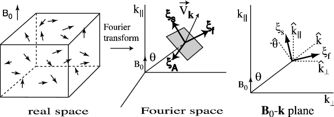
Figure 1: Separation method. We separate Alfven, slow, and fast modes in Fourier space by projecting the velocity Fourier component ${\bf v_{k}}$ onto bases ${\bf\xi}_{A}$, ${\bf\xi}_{s}$, and ${\bf\xi}_{f}$, respectively. Note that ${\bf\xi}_{A}=-\hat{\bf\varphi}$. Slow basis ${\bf\xi}_{s}$ and fast basis ${\bf\xi}_{f}$ lie in the plane defined by ${\bf B}_{0}$ and ${\bf k}$. Slow basis ${\bf\xi}_{s}$ lies between $-\hat{\bf\theta}$ and $\hat{\bf k}_{\|}$. Fast basis ${\bf\xi}_{f}$ lies between $\hat{\bf k}$ and $\hat{\bf k}_{\perp}$.

Let us start with a discussion why isotropic Kolmogorov turbulence cannot be applicable for describing strongly magnetized gas. Assume that, at some large scale $L$, the magnetic energy and kinetic energy are equal: $\rho V_{L}^{2}/2\sim B^{2}/(4\pi)$. According to the Kolmogorov theory, the kinetic energy at scale $l<L$ is $\rho V_{l}^{2}/2\sim(l/L)^{2/3}(\rho V_{L}^{2}/2)$, which is smaller than the large scale kinetic energy by a factor of $(l/L)^{2/3}$. But, magnetic energy density does not diminish as the scale reduces. Therefore, at scales smaller than $L$, hydrodynamic motions will not be able to bend magnetic field lines substantially.

An important observation that leads to understanding of the GS95 scaling is that magnetic field cannot prevent mixing motions of magnetic field lines if the motions are perpendicular to the magnetic field. Those motions will cause, however, waves that will propagate along magnetic field lines. If that is the case, the time scale of the wave-like motions, i.e. $\sim l_{\|}/V_{A}$, where $l_{\|}$ is the characteristic size of the perturbation along the magnetic field and $V_{A}=B/\sqrt{4\pi\rho}$ is the local Alfven speed, will be equal to the hydrodynamic time-scale, $l_{\perp}/v_{l}$, where $l_{\perp}$ is the characteristic size of the perturbation perpendicular to the magnetic field. The mixing motions are hydrodynamic-like and therefore obey Kolmogorov scaling $v_{l}\propto l_{\perp}^{1/3}$. Combining the two relations above we can get the GS95 anisotropy, $l_{\|}\propto l_{\perp}^{2/3}$ (or $k_{\|}\propto k_{\perp}^{2/3}$ in terms of wave-numbers). If we interpret $l_{\|}$ as the eddy size in the direction of the local magnetic field and $l_{\perp}$ as that in the perpendicular directions, the relation implies that smaller eddies are more elongated (see Appendix B for illustration of scale-dependent anisotropy).

How is this idealized incompressible model related to the actual, e.g. interstellar, turbulence? Compressible MHD turbulence is a highly non-linear phenomenon and it has been thought that different types of perturbations or modes (Alfven, slow and fast) in compressible media are strongly coupled. Nevertheless, one may question whether this is true. A remarkable feature of the GS95 model is that Alfven perturbations cascade to small scales over just one wave period, while the other non-linear interactions require more time. Therefore one might expect that the non-linear interactions with other types of waves should affect Alfvenic cascade only marginally. Moreover, as the Alfven waves are incompressible, the properties of the corresponding cascade may not depend on the sonic Mach number.

The generation of compressible motions (i.e. radial components in Fourier space) from Alfvenic turbulence is a measure of mode coupling. How much energy in compressible motions is drained from Alfvenic cascade? According to the closure calculations (Bertoglio, Bataille, & Marion 2001; see also Zank & Matthaeus 1993), the energy in compressible modes in hydrodynamic turbulence scales as $\sim M_{s}^{2}$ if $M_{s}<1$. We may conjecture that this relation can be extended to MHD turbulence if, instead of $M_{s}^{2}$, we use $\sim(\delta V)_{A}^{2}/(a^{2}+V_{A}^{2})$. (Hereinafter, we define $V_{A}\equiv B_{0}/\sqrt{4\pi\rho}$, where $B_{0}$ is the mean magnetic field strength.) However, as the Alfven modes are anisotropic, this formula may require an additional factor. The compressible modes are generated inside the so-called Goldreich-Sridhar cone, which takes up $\sim(\delta V)_{A}/V_{A}$ of the wave vector space. The ratio of compressible to Alfvenic energy inside this cone is the ratio given above. If the generated fast modes become isotropic (see below), the diffusion or, “isotropization” of the fast wave energy in the wave vector space increase their energy by a factor of $\sim V_{A}/(\delta V)_{A}$. This results in

$$\frac{(\delta V)_{rad}^{2}}{(\delta V)_{A}^{2}}\la\left[\frac{V_{A}^{2}+a^{2}}{(\delta V)^{2}_{A}}\frac{(\delta V)_{A}}{V_{A}}\right]^{-1},$$ (1)

where $(\delta V)_{rad}^{2}$ and $(\delta V)_{A}^{2}$ are energy of compressible and Alfven modes, respectively. Eq. (1) suggests that the drain of energy from Alfvenic cascade is marginal when the amplitudes of perturbations are weak, i.e. $(\delta V)_{A}\ll V_{A}$.

If Alfven cascade evolves on its own, it is natural to assume that slow modes exhibit the GS95 scaling. Indeed, slow modes in gas pressure dominated environment (high $\beta$ plasmas) are similar to the pseudo-Alfven modes in incompressible regime (see GS95; Lithwick & Goldreich 2001). The latter modes do follow the GS95 scaling. In magnetic pressure dominated environments (low $\beta$ plasmas), slow modes are density perturbations propagating with the sound speed $a$ parallel to the mean magnetic field (see equation (69)). Those perturbations are essentially static for $a\ll V_{A}$. Therefore Alfvenic turbulence is expected to mix density perturbations as if they were passive scalar. This also induces GS95 spectrum.

The fast waves in low $\beta$ regime propagate at $V_{A}$ irrespectively of the magnetic field direction. In high $\beta$ regime, the properties of fast modes are similar, but the propagation speed is the sound speed $a$. Thus the mixing motions induced by Alfven waves should marginally affect the fast wave cascade. It is expected to be analogous to the acoustic wave cascade and hence be isotropic.

For most part of this paper, we shall assumed that $\delta V\sim\delta B/\sqrt{4\pi\rho}\sim B_{0}/\sqrt{4\pi\rho}$, where $\delta B$ is the r.m.s. strength of the random magnetic field. This is less restrictive than it might appear, since as long as there is some scale $l^{\prime}$ in the turbulent cascade where $v_{l^{\prime}}\sim B/\sqrt{4\pi\rho}$ we can take $L=l^{\prime}$, $V_{L}=v_{l^{\prime}}$ and use this model of turbulence for all smaller scales. Suppose that we have a turbulent system initially threaded by a mean magnetic field only. If initially the turbulent energy is larger than the magnetic energy of the mean field, we are in the regime of so-called superAlfvenic turbulence. In this regime the growth of the magnetic field is expected through so called “turbulent dynamo” (see Batchelor 1950; Brandenburg et al. 1996; Cho & Vishniac 2000a). Initially, the growth of magnetic energy is most active at the scale roughly an order of magnitude larger than the dissipation scale and the magnetic spectrum peaks at the scale. As the magnetic energy grows, the magnetic back reaction becomes important at the scale and the peak of the magnetic power spectrum moves to larger scales. Finally, when equipartition between the kinetic and magnetic energy densities occurs at a scale somewhat (factor of 2 or 3) smaller than the kinetic energy peak, turbulence reaches a statistically stationary state. This agrees well with the results of incompressible simulations in Cho & Vishniac (2000a). However, this is not universally accepted idea. For example, Padoan & Nordlund (1999) reported that, in their compressible simulations, the power spectrum of $\rho^{1/2}v$ has a shallower slope then those of velocity and magnetic field, which implies that equipartition between kinetic magnetic energy cannot be reached at small scales. At scales smaller than the equipartition scale, the turbulence becomes subAlfvenic and our earlier considerations should be applicable.

The arguments above suggest that compressible MHD turbulence should demonstrate well defined scaling relations. Below we test those arguments and reveal scaling relations for different $\beta$s and Mach numbers.

Figure 2: Mode coupling studies. (a)left: Square of the r.m.s. velocity of the compressible modes. We use $144^{3}$ grid points. Only Alfven modes are allowed as the initial condition. “Pluses” are for low $\beta$ cases ($0.02\leq\beta\leq 0.4$). “Diamonds” are for high $\beta$ cases ($1\leq\beta\leq 20$). (b)middle: Generation of fast modes. Snapshot is taken at t=0.06 from a simulation (with $144^{3}$ grid points) that started off with Alfven modes only. Initially, $\beta$ (ratio of gas to magnetic pressure, $P_{g}/P_{mag}$) $=0.2$ and $M_{s}$ (sonic Mach number) $\sim 1.6$. (c)right: Comparison of decay rates. Decay of Alfven modes is not much affected by other (slow and fast) modes. We use $216^{3}$ grid points. Initially, $\beta=0.02$ and $M_{s}\sim 4.5$ for the solid line and $M_{s}\sim 7$ for the dotted line. Note that initial data are, in some sense, identical for the solid and the dotted lines. The sonic Mach number for the solid line is smaller because we removed fast and slow modes from the initial data before the decay simulation. For the dotted line, we did not remove any modes from the initial data.

2.2 Numerical scheme

We use a third-order accurate hybrid essentially non-oscillatory (ENO) scheme (see CL02) to solve the ideal isothermal MHD equations in a periodic box:

$${\partial\rho}/{\partial t}+\nabla\cdot(\rho{\bf v})=0,$$ (2)

$${\partial{\bf v}}/{\partial t}+{\bf v}\cdot\nabla{\bf v}+\rho^{-1}\nabla(a^{2}\rho)-(\nabla\times{\bf B})\times{\bf B}/4\pi\rho={\bf f},$$ (3)

$${\partial{\bf B}}/{\partial t}-\nabla\times({\bf v}\times{\bf B})=0,$$ (4)

with $\nabla\cdot{\bf B}=0$ and an isothermal equation of state. Here $\bf{f}$ is a random large-scale driving force, $\rho$ is density, ${\bf v}$ is the velocity, and ${\bf B}$ is magnetic field. The rms velocity $\delta V$ is maintained to be approximately unity (in fact $\delta V\sim 0.7$), so that ${\bf v}$ can be viewed as the velocity measured in units of the r.m.s. velocity of the system and ${\bf B}/\sqrt{4\pi\rho}$ as the Alfvén velocity in the same units. The time $t$ is in units of the large eddy turnover time ($\sim L/\delta V$) and the length in units of $L$, the scale of the energy injection. The magnetic field consists of the uniform background field and a fluctuating field: ${\bf B}={\bf B}_{0}+{\bf b}$.

For mode coupling studies (Fig. 2), we do not drive turbulence. For scaling studies, we drive turbulence solenoidally in Fourier space and use $216^{3}$ points, $V_{A}=B_{0}/\sqrt{4\pi\rho}=1$, and $\rho_{0}=1$. The average rms velocity in statistically stationary state is $\delta V\sim 0.7$.

For our calculations we assume that $B_{0}/\sqrt{4\pi\rho}\sim\delta B/\sqrt{4\pi\rho}\sim\delta V$. In this case, the sound speed is the controlling parameter and basically two regimes can exist: supersonic and subsonic. Note that supersonic means low-beta and subsonic means high-beta. When supersonic, we consider mildly supersonic (or, mildly low-$\beta$) and highly supersonic (or, very low-$\beta$).

2.3 Separation of MHD modes

Three types of waves exist (Alfven, slow and fast) in compressible magnetized plasma. The slow, fast, and Alfven bases that denote the direction of displacement vectors for each mode are given by

$$\hat{\bf\xi}_{s}\propto(-1+\alpha-\sqrt{D})k_{\|}\hat{\bf k}_{\|}+(1+\alpha-\sqrt{D})k_{\perp}\hat{\bf k}_{\perp},$$ (5)

$$\hat{\bf\xi}_{f}\propto(-1+\alpha+\sqrt{D})k_{\|}\hat{\bf k}_{\|}+(1+\alpha+\sqrt{D})k_{\perp}\hat{\bf k}_{\perp},$$ (6)

$$\hat{\bf\xi}_{A}=-\hat{\bf\varphi}=\hat{\bf k}_{\perp}\times\hat{\bf k}_{\|},$$ (7)

where $D=(1+\alpha)^{2}-4\alpha\cos\theta$, $\alpha=a^{2}/V_{A}^{2}=\beta(\gamma/2)$, $\theta$ is the angle between ${\bf k}$ and ${\bf B}_{0}$, and $\hat{\bf\varphi}$ is the azimuthal basis in the spherical polar coordinate system. These are equivalent to the expression in CL02:

$$\hat{\bf\xi}_{s} \propto k_{\|}\hat{\bf k}_{\|}+\frac{1-\sqrt{D}-{\beta}/2}{1+\sqrt{D}+{\beta}/2}\left[\frac{k_{\|}}{k_{\perp}}\right]^{2}k_{\perp}\hat{\bf k}_{\perp},$$ (8)

$$\hat{\bf\xi}_{f} \propto \frac{1-\sqrt{D}+{\beta}/2}{1+\sqrt{D}-{\beta}/2}\left[\frac{k_{\perp}}{k_{\|}}\right]^{2}k_{\|}\hat{\bf k}_{\|}+k_{\perp}\hat{\bf k}_{\perp}.$$ (9)

(Note that $\gamma=1$ for isothermal case.)

Slow and fast velocity components can be obtained by projecting velocity Fourier component ${\bf v}_{\bf k}$ onto $\hat{\bf\xi}_{s}$ and $\hat{\bf\xi}_{f}$, respectively. In Appendix A, we discuss how to separate slow and fast magnetic modes. We obtain energy spectra using this projection method. When we calculate the structure functions (e.g. for Alfvén velocity) in real space, we first obtain the Fourier components using the projection and, then, we obtain the real space values by performing Fourier transform.

Figure 3: Low $\beta$ ($\beta\sim 0.2$ and $M_{s}\sim$2.3). Scalings relations. Results from driven turbulence with $M_{A}$ (Alfven Mach number) $\sim 0.7$, and $216^{3}$ grid points. ($V_{A}\equiv B_{0}/\sqrt{4\pi\rho}=1$; $a$ (sound speed) $=\sqrt{0.1}$; $\delta V\sim 0.7$.) (a)Upper-left: Spectra of Alfvén modes follow a Kolmogorov-like power law. (b)Middle-left: The second-order structure function ($SF_{2}$) for velocity of Alfvén modes shows anisotropy similar to the GS95 ($r_{\|}\propto r_{\perp}^{2/3}$ or $k_{\|}\propto k_{\perp}^{2/3}$). The structure functions are measured in directions perpendicular or parallel to the local mean magnetic field in real space. We obtain real-space velocity and magnetic fields by inverse Fourier transform of the projected fields. (c)Lower-left: SF₂ on the parallel axis and on perpendicular axis for Alfven modes velocity. (d)Upper-middle: Spectra of slow modes also follow a Kolmogorov-like power law. (e)Middle-middle: Slow mode velocity shows anisotropy similar to the GS95. (f)Lower-middle: SF₂ on the parallel axis and on perpendicular axis for slow modes velocity. (g)Upper-right: Spectra of fast modes are compatible with the IK spectrum. (h)Upper-middle: The SF₂ of fast modes velocity shows isotropy. Fast mode magnetic field also shows isotropy. (i)Lower-right: SF₂ on the parallel axis and on perpendicular axis for fast modes velocity.

3 Velocity scalings

3.1 Mode coupling

Figure 4: High $\beta$ ($\beta\sim 4$ and $M_{s}\sim$0.35). $V_{A}\equiv B_{0}/\sqrt{4\pi\rho}=1$. $a$ (sound speed) $=\sqrt{2}$. $\delta V\sim 0.7$. See caption in Fig. 3. Alfven and slow modes follow the GS95 scalings. Fast modes are isotropic.

In CL02 we demonstrated the decoupling of Alfven and fast modes in low $\beta$ plasmas. Here we substantially extend the CL02 analysis. As mentioned above, the coupling of compressible and incompressible modes is crucial. If Alfvenic modes produce a copious amount of compressible modes, the whole picture of independent Alfvenic turbulence fails. However, our calculations show that the amount of energy drained into compressible motions is negligible, provided that either the external magnetic field or the gas pressure is sufficiently high. Fig. 2a suggests that the generation of compressible motions follows equation (1). Fast modes also follow a similar scaling, although the scatter is a bit larger. The marginal generation of compressible modes is in agreement with earlier studies by Boldyrev et al. (2002b) and Porter, Pouquet, & Woodward (2002), where the velocity was decomposed into a potential component and a solenoidal component. See Fig. 2a for the values of $\sim\chi$ (=the ratio of the mean square potential to solenoidal velocity). Fig. 2b demonstrates that fast modes are initially generated anisotropically, which supports our theoretical consideration in §2.1.

Fig. 2c shows that dynamics of Alfven modes is not affected by slow modes. We first perform a driven turbulence simulation with $216^{3}$ grid point, $\beta\sim 0.02$, and $M_{s}\sim 7$. Then, after it has reached a statistically stationary state, we stop the run and save the data. Using these data, we perform two decay simulations. For one (the solid line), we remove all slow and fast modes and let the turbulence decay. For the other (the dotted line), without removing any modes, we just let the turbulence decay. The solid line in the figure is the energy in Alfven modes when we start the decay simulation with Alfven modes only. The dotted line is the Alfven energy when we start the simulation with all modes. This result confirms that Alfven modes cascade is almost independent of slow and fast modes. In this sense, coupling between Alfven and other modes is weak.

3.2 High-$\beta$ and mildly supersonic low-$\beta$ regimes

Alfvén Modes.— Fig. 3a (low-$\beta$) and Fig. 4a (high-$\beta$) show that the power spectra of Alfvén waves follow a Kolmogorov spectrum:

$$\mbox{\it Spectrum of Alfv\'{e}n Waves:~{}~{}~{}}E^{A}(k)\propto k_{\perp}^{-5/3}.$$ (10)

In Fig. 3b (middle-left panel) and Fig. 4b (middle-left panel), we plot contours of equal second-order structure function for velocity ($SF_{2}({\bf r})=<|{\bf v}({\bf x}+{\bf r})-{\bf v}({\bf x})|^{2}>_{avg.~{}over~{}{\bf x}}$) obtained in local coordinate systems in which the parallel axis is aligned with the local mean field (see Cho & Vishniac 2000b; CLV02a; Maron & Goldreich 2001). The $SF_{2}$ along the axis perpendicular to the local mean magnetic field follows a scaling compatible with $r^{2/3}$. The $SF_{2}$ along the axis parallel to the local mean field follows steeper $r^{1}$ scaling (Fig. 3c and Fig. 4c: lower-left panels). The results show reasonable agreement with the GS95 model for incompressible MHD turbulence,

$$\mbox{\it Anisotropy of Alfv\'{e}n Waves:~{}~{}~{}}r_{\|}\propto r_{\perp}^{2/3},\mbox{~{}or~{}}k_{\|}\propto k_{\perp}^{2/3},$$ (11)

where $r_{\|}$ and $r_{\perp}$ are the semi-major axis and semi-minor axis of eddies, respectively (Cho & Vishniac 2000b).

Slow waves.— The incompressible limit of slow waves is pseudo-Alfvén waves. Goldreich & Sridhar (1997) argued that the pseudo-Alfvén waves are slaved to the shear-Alfvén (i.e. ordinary Alfvén) waves, which means that pseudo-Alfvén modes do not cascade energy for themselves. Lithwick & Goldreich (2001) made similar theoretical arguments for high $\beta$ plasmas and conjectured similar behaviors of slow modes in low $\beta$ plasmas. We confirmed that similar arguments are also applicable to slow waves in low $\beta$ plasmas (CL02). Indeed, power spectra in Fig. 3d and Fig. 4d (upper-middle panels) are consistent with:

$$\mbox{\it Spectrum of Slow Modes:~{}~{}~{}}E^{s}(k)\propto k_{\perp}^{-5/3}.$$ (12)

In Fig. 3e and Fig. 4e (middle-middle panels), contours of equal second-order velocity structure function ($SF_{2}$), representing eddy shapes, show scale-dependent anisotropy: smaller eddies are more elongated. The results show reasonable agreement with the GS95-type anisotropy

$$\mbox{\it Anisotropy of Slow Modes:~{}~{}~{}}k_{\|}\propto k_{\perp}^{2/3},\mbox{~{}or~{}}r_{\|}\propto r_{\perp}^{2/3},$$ (13)

where $r_{\|}$ and $r_{\perp}$ are the semi-major axis and semi-minor axis of eddies, respectively.

Figure 5: Highly supersonic low $\beta$ ($\beta\sim 0.02$ and $M_{s}\sim$7). $V_{A}\equiv B_{0}/\sqrt{4\pi\rho}=1$. $a$ (sound speed) $=0.1$. $\delta V\sim 0.7$. Alfven modes follow the GS95 scalings. Slow modes follow the GS95 anisotropy. But velocity spectrum of slow modes is uncertain. Fast modes are isotropic.

Fast waves.— Fig. 3h and Fig. 4h (middle-right panels) show fast modes are isotropic. The resonance conditions for the interacting fast waves are $\omega_{1}+\omega_{2}=\omega_{3}\mbox{~{}~{}and~{}~{}}{\bf k}_{1}+{\bf k}_{2}={\bf k}_{3}.$ Since $\omega\propto k$ for the fast modes, the resonance conditions can be met only when all three ${\bf k}$ vectors are collinear. This means that the direction of energy cascade is radial in Fourier space. This is very similar to acoustic turbulence, turbulence caused by interacting sound waves (Zakharov 1967; Zakharov & Sagdeev 1970; L’vov, L’vov, & Pomyalov 2000). Zakharov & Sagdeev (1970) found $E(k)\propto k^{-3/2}$. However, there is debate about the exact scaling of acoustic turbulence. Here we cautiously claim that our numerical results are compatible with the Zakharov & Sagdeev scaling:

$$\mbox{\it Spectrum of Fast Modes:~{}~{}~{}}E^{f}(k)\sim k^{-3/2}.$$ (14)

The eddies are isotropic (see also Appendix B).

3.3 Highly supersonic low-$\beta$ case

The results for low-$\beta$ in the previous subsection are for a Mach number of $\sim 2.3$. In this subsection, we present results for a Mach number of $\sim 7$. Obviously shock formation is faster when the Mach number of the system is high. We also expect that turbulent motions can compress/disperse the gas more easily when the Mach number is high. As a result, we expect higher density fluctuations when Mach number is higher. Thus we check the scaling relations for high Mach number fluids.

Fig. 5 shows that most of the scaling relations that hold true in mildly supersonic flows are still valid in the highly supersonic case. Especially anisotropy of Alfven, slow, and fast modes is almost identical to the one in the previous section. However, the power spectra for slow modes do not show the Kolmogorov slope. The slope is close to $-2$, which is suggestive of shock formation. At this moment, it is not clear whether or not the $-2$ slope is the true slope. In other words, the observed $-2$ slope might be due to the limited numerical resolution. Runs with higher numerical resolution should give the definite answer.

3.4 SuperAlfvenic turbulence

Figure 6: Super-Alfvenic turbulence ($M_{A}\sim 8$ and $M_{s}\sim 2.5$). $V_{A}\equiv B_{0}/\sqrt{4\pi\rho}=0.1$. $a$ (sound speed) $=\sqrt{0.1}$. $\delta V\sim 0.8$. (a)left: Spectra. (b)middle: VSF₂. (c)right: BSF₂. No mode decomposition is used for (b) and (c).

Figure 7: Comparison between Fourier space method and real space method. (a)left: From real space calculation. $M_{s}\sim 7$. (b)middle: Solid: Fourier space. Dashed: real space. $M_{s}\sim 7$. (c)right: Similar plot for $M_{s}\sim$ 2.3.

So far we considered “sub-Alfvenic” turbulence in which the Alfven speed associated with the mean magnetic field is slightly faster than the r.m.s. fluid velocity. If the opposite case is true (i.e. if the mean field $B_{0}$ is weak), the turbulence is called “super-Alfvenic”. In super-Alfvenic turbulence, large scale magnetic field lines can show very chaotic structures. Whether or not the ISM turbulence is sub-Alfvenic is still a controversial issue.

We mentioned in §2.1 that, even in the case of super-Alfvenic turbulence, we can find some scale $l^{\prime}$ in the turbulent cascade where $v_{l^{\prime}}\sim B/\sqrt{4\pi\rho}$ and we can apply our model of sub-Alfvenic turbulence for all smaller scales. Fig. 6 supports this idea. The contours in the figure are the second order structure functions (SF₂) of velocity and magnetic field. We do not use mode decomposition. Nevertheless, the velocity SF₂ reflects scalings of Alfven and slow modes, because fast modes are weaker than Alfven and slow modes. As expected, anisotropy emerges at small scales. This is very similar to incompressible case (Cho & Vishniac 2000a).

Fig. 6(a) shows power spectra. We notice that the power spectra of velocity and magnetic field have different shapes. The velocity power spectrum is larger than the magnetic one near the energy injection scale at $k\sim 2.5$. However, for larger k’s ($k>6$), the magnetic power spectrum is larger than the velocity one. This behavior is well known in incompressible simulations with unit magnetic Prandtl number (see, for example, Kida, Yanase, & Mizushima 1991; Cho & Vishniac 2000a). A similar behavior is also observed in earlier compressible simulations (see, for example, Brandenburg et al. 1996). Cho & Vishniac (2000a) argued that the transition from $E_{v}(k)>E_{b}(k)$ to $E_{v}(k)<E_{b}(k)$ occurs at a wavelength 2 or 3 time larger than that of the energy injection scale.

A careful look at Fig. 6(a) reveals that, for $k<8$, the power spectrum of velocity declines faster than Kolmogorov as $k$ increases. This is not very surprising because magnetic field has more power than velocity at large k’s and, therefore, can affect the velocity power spectrum at small k’s. Kida et al. (1991) claimed that the sum of $E_{v}(k)+E_{b}(k)$ roughly follows Kolmogorov spectrum in their incompressible simulations. If this is true, then the velocity power spectrum should have a spectrum steeper than Kolmogorov at small k’s because many simulations have shown that the magnetic power spectrum is significantly flatter than the velocity one at small k’s when the mean field $B_{0}$ is weak (Kida et al. 1991; Brandenburg et al. 1996; Cho & Vishniac 2000a). After $k\sim 8$, it seems that the velocity power spectrum gets flatter.

Boldyrev, Nordlund, & Padoan (2002a) also obtained velocity power spectrum steeper than Kolmogorov in their supersonic super-Alfvenic MHD simulations. They attributed the steep spectrum to different intermittency properties compared to the incompressible case. Since they used a different simulation set-up, we do not directly compare our results and theirs. For example, their turbulence is driven at larger scales than ours and their sonic Mach number is larger than ours. Further parameter study is absolutely necessary.

3.5 How good is our technique?

The technique described in §2.3 is statistical in nature. That is, we separate each MHD mode with respect to the mean magnetic field ${\bf B}_{0}$. This procedure is affected by the wandering of large scale magnetic field lines, as well as density inhomogeneities.

Nevertheless, we can show that our technique gives statistically correct results. In low $\beta$ regime, the velocity of a slow mode is nearly parallel to the local mean magnetic field. Therefore, for low $\beta$ plasmas, we can obtain velocity statistics for slow modes in real space as follows. First, we identify the direction of the local mean magnetic field using the method described in Cho & Vishniac (2000b). Second, we calculate the second order structure function for slow modes by the formula vSF${}_{2}({\bf r})=<|\left({\bf v}({\bf x}+{\bf r})-{\bf v}({\bf x})\right)\cdot\hat{\bf B}_{l}|^{2}>$, where $\hat{\bf B}_{l}$ is the unit vector along the local mean field.

Fig. 7(a) shows the contours obtained by the method for the high Mach number run. In Fig. 7(b), we compare the result obtained this way (dashed lines) and our technique described in §2.3 (solid lines). We also show a similar plot for the mildly supersonic case in Fig. 7(c). These results confirm that the method described in §2.3 gives statistically correct scaling relations.

4 Linear Estimates of Density and Magnetic Field Fluctuations

Figure 8: Density structures. (a)left: $M_{s}\sim 0.35$ (high $\beta$). (b)middle: $M_{s}\sim 2.3$ (mildly supersonic low $\beta$). (c)right: $M_{s}\sim 7$ (highly supersonic low $\beta$).

In this section, we estimate the magnitude of the r.m.s. fluctuations of magnetic field and density. Figures 3, 4, and 5 show that magnetic field and density have spectral indexes similar to those of velocity. We also expect that isotropy/anisotropy of magnetic field is similar to that of velocity. Therefore, we do not discuss these quantities here. However, anisotropy of density shows different behavior. Fig. 8 shows structure of density. Density shows anisotropy for the high $\beta$ case. But, for low $\beta$ cases, density shows more or less isotropic structures. We suspect that shock formation is responsible for the isotropization of density.

To estimate the r.m.s. fluctuations, we use the following linearized continuity and induction equations:

$$|\rho_{k}| = (\rho_{0}v_{k}/c)|\hat{\bf k}\cdot\hat{\bf\xi}|,$$ (15)

$$|b_{k}| = (B_{0}v_{k}/c)|\hat{\bf B}_{0}\times\hat{\bf\xi}|,$$ (16)

where $c$ denotes propagation speed of slow or fast wave (equation (60)). From this, we obtain the r.m.s. fluctuations

$$(\delta\rho/\rho_{0})_{s} = (\delta V)_{s}\langle|\hat{\bf k}\cdot\hat{\bf\xi}_{s}/c_{s}|\rangle,$$ (17)

$$(\delta\rho/\rho_{0})_{f} = (\delta V)_{f}\langle|\hat{\bf k}\cdot\hat{\bf\xi}_{f}/c_{f}|\rangle,$$ (18)

$$(\delta B/B_{0})_{s} = (\delta V)_{s}\langle|\hat{\bf B}_{0}\times\hat{\bf\xi}_{s}/c_{s}|\rangle,$$ (19)

$$(\delta B/B_{0})_{f} = (\delta V)_{f}\langle|\hat{\bf B}_{0}\times\hat{\bf\xi}_{f}/c_{f}|\rangle,$$ (20)

where angled brackets denote a proper Fourier space average. Generation of slow and fast modes velocity ($(\delta V)_{s}$ and $(\delta V)_{f}$) depends on driving force. Therefore, we may simply assume that

$$(\delta V)_{A}\sim(\delta V)_{s}\sim(\delta V)_{f},$$ (21)

where we ignore constants of order unity. However, when we consider mostly incompressible driving, the generation of fast modes follows equation (1). In this case, the amplitude of fast mode velocity is reduced by a factor of $\left[\frac{V_{A}^{2}+a^{2}}{(\delta V)^{2}_{A}}\frac{(\delta V)_{A}}{V_{A}}\right]^{-1/2}$:

$$(\delta V)_{A}\sim(\delta V)_{s}\sim\left[\frac{V_{A}^{2}+a^{2}}{(\delta V)^{2}_{A}}\frac{(\delta V)_{A}}{V_{A}}\right]^{1/2}(\delta V)_{f}.$$ (22)

When we assume $(\delta V)_{A}\sim V_{A}$, equation (22) reduces to equation (21) in low $\beta$ plasmas.

4.1 Low-$\beta$ case

In this limit, $c_{s}\sim a\cos\theta$ and $c_{f}\sim V_{A}$. Using equations (69) and (70), we obtain

$$(\delta\rho/\rho_{0})_{s} \sim (\delta V)_{s}\langle|\cos\theta/c_{s}|\rangle\sim(\delta V)_{s}/a,$$ (23)

$$(\delta\rho/\rho_{0})_{f} = (\delta V)_{f}\langle|\sin\theta/c_{f}|\rangle\sim(\delta V)_{f}/V_{A},$$ (24)

$$(\delta B/B_{0})_{s} = (\delta V)_{s}\langle|\alpha\cos\theta\sin\theta/c_{s}|\rangle\sim\alpha(\delta V)_{s}/a,$$ (25)

$$(\delta B/B_{0})_{f} = (\delta V)_{f}\langle|1/c_{f}|\rangle\sim(\delta V)_{f}/V_{A},$$ (26)

where we ignore $\cos\theta$’s or $\sin\theta$’s.

When we assume $(\delta V)_{A}\sim(\delta V)_{s}\sim(\delta V)_{f}\sim V_{A}$, we get

$$(\delta\rho/\rho_{0})_{s} \sim M_{s},$$ (27)

$$(\delta\rho/\rho_{0})_{f} = \sqrt{\beta}M_{s},$$ (28)

$$(\delta B/B_{0})_{s} = \beta M_{s},$$ (29)

$$(\delta B/B_{0})_{f} = \sqrt{\beta}M_{s}$$ (30)

Therefore, in low $\beta$ plasmas, slow modes give rise to most of density fluctuations (CL02). On the other hand, magnetic fluctuation by slow modes is smaller than that by fast modes by a factor of $\sqrt{\beta}$.

4.2 High-$\beta$ case

In this limit, $c_{s}\sim V_{A}\cos\theta$ and $c_{f}\sim a$. Using equations (71) and (72), we obtain

$$(\delta\rho/\rho_{0})_{s} \sim (\delta V)_{s}\langle|\cos\theta\sin\theta/(\alpha c_{s})|\rangle$$ (31)

$$\sim (V_{A}/a)(\delta V)_{s}/a,$$

$$(\delta\rho/\rho_{0})_{f} = (\delta V)_{f}\langle|1/c_{f}|\rangle\sim(\delta V)_{f}/a,$$ (32)

$$(\delta B/B_{0})_{s} = (\delta V)_{s}\langle|\cos\theta/c_{s}|\rangle\sim(\delta V)_{s}/V_{A},$$ (33)

$$(\delta B/B_{0})_{f} = (\delta V)_{f}\langle|\sin\theta/c_{f}|\rangle\sim(\delta V)_{f}/a,$$ (34)

where we ignore $\cos\theta$’s or $\sin\theta$’s.

Let us just assume that $(\delta V)_{A}\sim(\delta V)_{s}\sim V_{A}\sim M_{s}^{-1}(\delta V)_{f}$ (cf. equation (22)). Then we have

$$(\delta\rho/\rho_{0})_{s} \sim M_{s}/\sqrt{\beta}\sim M_{s}^{2},$$ (35)

$$(\delta\rho/\rho_{0})_{f} \sim M_{s}^{2},$$ (36)

$$(\delta B/B_{0})_{s} = O(1),$$ (37)

$$(\delta B/B_{0})_{f} = M_{s}^{2}.$$ (38)

The density fluctuation associated with slow modes is $\sim M_{s}^{2}$, when $(\delta V)_{s}\sim(\delta V)_{A}\sim V_{A}$. This is consistent with Zank & Matthaeus (1993). The ratio of $(\delta\rho)_{s}$ to $(\delta\rho)_{f}$ is of order unity. Therefore, both slow and fast modes give rise to similar amount of density fluctuations. Note that this argument is of order-of-magnitude in nature. In fact, in our simulations for the high $\beta$ case, the r.m.s. density fluctuation by slow modes is about twice as large as that by fast modes. When we use equation (21), we have a different result: $(\delta\rho)_{s}\sim(V_{A}/a)(\delta\rho)_{f}<(\delta\rho)_{f}$. It is obvious that slow modes dominate magnetic fluctuations: $(\delta B)_{s}>(\delta B)_{f}$ for both equations (21) and (22).

5 Viscosity-damped Regime of MHD Turbulence

In hydrodynamic turbulence viscosity sets a minimal scale for motion, with an exponential suppression of motion on smaller scales. Below the viscous cutoff the kinetic energy contained in a wavenumber band is dissipated at that scale, instead of being transferred to smaller scales. This means the end of the hydrodynamic cascade, but in MHD turbulence this is not the end of magnetic structure evolution. For viscosity much larger than resistivity, $\nu\gg\eta$, there will be a broad range of scales where viscosity is important but resistivity is not. On these scales magnetic field structures will be created by the shear from non-damped turbulent motions, which amounts essentially to the shear from the smallest undamped scales. The created magnetic structures would evolve through generating small scale motions. As a result, we expect a power-law tail in the magnetic energy distribution, rather than an exponential cutoff. Cho, Lazarian, & Vishniac (CLV02b) performed numerical simulations of turbulence in this regime threaded by a strong ($B_{0}/\sqrt{4\pi\rho}\sim\delta V$) mean magnetic field and reported that this regime possesses completely different scaling relations and anisotropic structures compared with ordinary MHD turbulence. Further research showed that there is a smooth connection between this regime and small scale turbulent dynamo in high magnetic Prandtl number fluids (see Schekochihin et al. 2002).

Figure 9: Viscous damped regime (viscosity $>$ magnetic diffusivity). Due to large viscosity, velocity damps after $k\sim 10$. (a) Left: Incompressible case with $384^{3}$ grid points. Magnetic spectra show a shallower slope ($E_{b}(k)\propto k^{-1}$) below the velocity damping scale. We achieve a very small magnetic diffusivity through the use hyper-diffusion. From Cho, Lazarian, & Vishniac (2002b). (b) Right: Compressible case with $216^{3}$ grid points. Magnetic and density spectra show structures below the velocity damping scale at $k\sim 10$. The structures are less obvious than the incompressible case because it is relatively hard to achieve very small magnetic diffusivity in the compressible run.

In partially ionized gas neutrals produce viscous damping of turbulent motions. In the Cold Neutral Medium (see Draine & Lazarian 1999 for a list of the idealized phases) this produces damping on the scale of a fraction of a parsec. The magnetic diffusion in those circumstances is still negligible and exerts an influence only at the much smaller scales, $\sim 100km$. Therefore, there is a large range of scales where the physics of the turbulent cascade is very different from the conventional MHD turbulence picture.

CLV02b explored this regime numerically with a grid of $384^{3}$ and a physical viscosity for velocity damping. The kinetic Reynolds number was around 100. We achieved a very small magnetic diffusivity by the use of hyper-diffusion. The result is presented in Fig. 9a. A theoretical model for this regime and its consequences for stochastic reconnection (Lazarian & Vishniac 1999) can be found in Lazarian, Vishniac, & Cho (2003). It explains the spectrum $E(k)\sim k^{-1}$ as a cascade of magnetic energy to small scales under the influence of shear at the marginally damped scales. The spectrum is similar to that of the viscous-convective range of passive scalar in hydrodynamic turbulence (see, for example, Batchelor 1959; Lesieur 1990), although the study in Lazarian, Vishniac, & Cho (2003) suggests that the physical origin of it is different. A study confirming that the $k^{-1}$ spectrum is not a bottleneck effect is presented in Cho, Lazarian, & Vishniac (2003b). The mechanism is based on the solenoidal motions and therefore the compressibility should not alter the physics of this regime of turbulence.

We show our results for the compressible fluid in Fig 9b. We use the same physical viscosity as in incompressible case (see CLV02b). We rely on numerical diffusion, which is much smaller than physical viscosity, for magnetic field. The inertial range is much smaller due to numerical reasons, but it is clear that the viscosity-damped regime of MHD turbulence persists. The magnetic fluctuations, however, compress the gas and thus cause fluctuations in density. This is a new (although expected) phenomenon compared to our earlier incompressible calculations. These density fluctuations may have important consequences for the small scale structure of the ISM.

6 Astrophysical Implications of Our Results

6.1 Parameter range explored

Parameters of astrophysical plasmas differ substantially for different astrophysical systems: from extremely high $\beta$ to extremely low $\beta$. Turbulence in some systems is expected to be superAlfvenic, in others it is expected to be subAlfvenic. Moreover, there is an ongoing controversy on what to expect and where. For instance, while high $\beta$ was considered a default for many phases of Milky Way ISM, recent observations by Beck (2002) suggest that the plasmas there may be low $\beta$. Therefore it is essential to have clear understanding of MHD turbulence for as large parameter space as possible.

SuperAlfvenic regime.— We have argued above that the difference between superAlfvenic and subAlfvenic turbulence is not as substantial as it is frequently thought. The difference between the two regimes stems from ratio of magnetic field to kinetic energies. However, as we mentioned in §2, if kinetic energy density exceed magnetic field energy density, the hydromagnetic motions drive turbulent dynamo. This enhances magnetic field energy density up to approximately equipartition value. Thus the difference between the superAlfvenic and subAlfvenic regimes amounts not to the energy of the magnetic field, but to the global level of field organization, e.g. to the magnetic field reversals etc. Our results in §3.4 suggest that the basic properties of the MHD turbulence in the subAlfvenic and superAlfvenic regimes are similar. This, however, does not preclude the intermittency of MHD turbulence being very different. The latter property can be tested using scalings of the higher order velocity correlations $SF_{p}({\bf r})\equiv\langle|{\bf v}({\bf x}+{\bf r})-{\bf v}({\bf x})|^{p}\rangle\propto r^{\zeta(p)}$. The corresponding scaling suggested by She-Leveque (1994) contains three parameters (see Politano & Pouquet 1995; Müller & Biskamp 2000): $g$ is related to the scaling $\delta v_{l}\sim l^{1/g}$, $x$ related to the energy cascade rate $t_{l}^{-1}\sim l^{-x}$, and C, the co-dimension of the dissipative structures:

$$\zeta(p)=p/g(1-x)+C\left(1-(1-x/C)^{p/g}\right).$$ (39)

Müller & Biskamp (2000) proposed that 3D incompressible MHD turbulence for zero mean field has Kolmogorov $g$ and $x$, while the the dissipation happens in the sheet-like structures, i.e. $C=3-2=1$. Using eq. (39) they obtained an excellent fit for their incompressible data. Later Boldyrev (2002) made the same assumption that $C=1$ (and same $g$ and $x$) for the compressible turbulence and Boldyrev, Nordlund, & Padoan (2002a) obtained an excellent fit to their compressible data. It appears surprising that incompressible MHD (Müller & Biskamp 2000) and supersonic compressible MHD (Boldyrev et al. 2002a) have similar intermittency structures. This issue is discussed in Cho, Lazarian, & Vishniac (2003b).

We would like to note, however, that our considerations about superAlfvenic turbulence are not applicable to the transient regimes when superAlfvenic motions are in the process of generating magnetic field and magnetic energy does not have time to come to a rough equipartition to the kinetic energy. Some parts of the ISM can well be in the transient regime for which temporary $\rho V^{2}/2\gg B^{2}/8\pi$.

$\beta=1$ case.— We provided theoretical considerations for both $\beta\gg 1$ and $\beta\ll 1$ cases. What about the intermediate cases of $\beta\sim 1$? Would the scaling of modes and mode coupling be different? To test this case we performed calculations for $\beta=1$. The results in Fig. 10 show that the scaling relations that hold true for mildly low $\beta$ regime are also applicable for $\beta=1$ regime.

Figure 10: $\beta=1$ case. (a)left: Alfven mode spectra. (b)second-left: Slow mode spectra. (c)second-right: Fast mode spectra. (d)right: Density structure.

6.2 Fundamental questions

How fast does MHD turbulence decay? This question has fundamental implications for star formation (see McKee 1999). Indeed, it was thought originally that magnetic fields would prevent turbulence from fast decay. Later (see Mac Low et al. 1998; Stone et al. 1998; and review by Vazquez-Semadeni et al. 2000) this was reported not to be true. However, fast decay was erroneously associated with the coupling between compressible and incompressible modes. The idea was that incompressible motions quickly transfer their energy to the compressible modes, which get damped fast by direct dissipation (presumably through shock formation).

Our calculations support the conjecture given by eq. (1). According to it the coupling of Alfven and compressible motions is important only at the energy injection scales where $\delta V_{l}\sim V_{A}$. As the turbulence evolves the perturbations become smaller and the coupling less efficient. Typically for numerical simulations the inertial range is rather small and this could explain why marginal coupling of modes was not noticed.

Our results show that MHD turbulence damping does not depend on whether the fluid is compressible or not. The incompressible motions damp also within one eddy turnover time. This is the consequence of the fact that within the strong turbulence mixing motions perpendicular to magnetic field are hydrodynamic to high order (CLV02a) and the cascade of energy induced by those motions is similar to the hydrodynamic one, i.e. energy cascade happens within an eddy turnover time.

The reported (see Mac Low et al. 1998) decay of the total energy of turbulent motions $E_{tot}$ follows $t^{-1}$ which can be understood if we account for the fact that the energy is being injected at the scale smaller than the scale of the system. Therefore some energy originally diffuses to larger scales through the inverse cascade. Our calculations stimulated by illuminating discussions with Chris McKee show that if this energy transfer is artificially prevented by injecting the energy on the scale of the computational box, the scaling of $E_{tot}$ becomes closer to $t^{-2}$.

Can compressible MHD turbulence decay slowly? Incompressible MHD computations (see Maron & Goldreich 2001; CLV02a) show that the rate of turbulence decay depends on the degree of turbulence imbalance, i.e. the difference in the energy fluxes moving in opposite directions. The strongly imbalanced incompressible turbulence was shown to persist longer than its balanced counterpart. This enabled CLV02a to speculate that this may enable energy transfer between clouds and may explain the observed turbulent linewidths of GMCs without evident star formation. Imbalanced turbulence can also make it possible to transfer energy from the galactic disk to heat the Reynolds layer (see Reynolds 1988).

Our results above show a marginal coupling of compressible and incompressible modes. This is suggestive that the results obtained in incompressible simulations are applicable to compressible environments if amplitudes of perturbations are not large. The complication arises from the existence of the parametric instability (Del Zanna, Velli, & Londrillo 2001) that happens as the density perturbations reflect Alfven waves and grow in amplitude. This instability eventually controls the degree of imbalance that is achievable. However, the growth rate of the instability is substantially slower than the Alfven wave oscillation rate. Therefore, if we take into account that interstellar sources are intermittent not only in space, but also in time, the transport of turbulent energy described in CLV02a seems feasible. Here we mention that the growth of the parametric instability described above may provide an alternative explanation for the observed infall motions of the cloud cores (Tafalla et al. 1998). Earlier those motions were explained as arising from linear damping of Alfven waves (Myers & Lazarian 1998).

Is the correlation between magnetic field and density tight in MHD turbulence? In the traditional static paradigm of the ISM, density and magnetic field increase simultaneously as clouds contract. Introduction of turbulence in the picture of ISM complicates the analysis (see discussion in Vazquez-Semadeni et al. 2000; CLV03a). Our results confirm earlier claims (e.g. Passot & Vazquez-Semadeni 2003) that magnetic field - density correlations may be weak. First of all, some magnetic field fluctuations are related to Alfvenic turbulence which does not compress the medium. Second, slow modes in low $\beta$ plasmas are essentially density perturbations that propagate along magnetic field and which marginally perturb magnetic fields. Moreover, our calculations (see Fig. 8) show that at substantially high Mach numbers the density correlations do not show anisotropies, while magnetic field fluctuations are anisotropic. On the basis of our calculations we might expect that the correlation may be a bit higher for high $\beta$ than for low $\beta$ plasmas.

Can viscously damped turbulence explain TSAS? The term “tiny-scale atomic structures” or TSAS was introduced by Heiles (1997) to describe the mysterious H I absorbing structures on scales from thousands to tens of AU, discovered by Dieter, Welch & Romney (1976). Analogs of TSAS are observed in NaI and CaII (Meyer & Blades 1996; Faison & Goss 2001; Andrews, Meyer, & Lauroesch 2001) and in molecular gas (Marscher, Moore, & Bania 1993).

Those structures can be produced by turbulence with a spectrum substantially more shallow than the Kolmogorov one, e.g. with the spectrum $E(k)\sim k^{-1}$ (see Deshpande 2000). Simulations in CLV02b and theoretical calculations in Lazarian, Vishniac & Cho (2003) show that the magnetic field in the viscosity-damped regime of MHD turbulence (see §5) can produce such a spectrum of magnetic fluctuations. Our calculations above are indicative that this will translate in the corresponding shallow spectrum of density. Our calculations are applicable on scales from the viscous damping scale (determined by equating the energy transfer rate with the viscous damping rate; $\sim 0.1$ pc in the Warm Neutral Medium with $n$ = 0.4 cm^-3, $T$= 6000 K) to the ion-neutral decoupling scale (the scale at which viscous drag on ions becomes comparable to the neutral drag; $\ll 0.1$ pc). Below the viscous scale the fluctuations of magnetic field obey the damped regime shown in Figure 9b and produce density fluctuations. For typical Cold Neutral Medium gas, the scale of neutral-ion decoupling decreases to $\sim 70$ AU, and is less for denser gas. TSAS may be created by strongly nonlinear MHD turbulence!

6.3 Application of the scaling laws obtained

Many astrophysical problems require some knowledge of the scaling properties of turbulence. Therefore we expect a wide range of applications of the established scaling relations. Here we discuss how our understanding of MHD turbulence affects a few selected issues.

As we mentioned in the introduction, the observations (see CLV03a for a review) indicate that interstellar spectrum exhibits Kolmogorov-type scaling $E(k)\sim k^{-5/3}$. On the basis of what we learned by now (see also Higdon 1983, GS95, Lithwick & Goldreich 2001, CL02) we may conclude that the MHD spectrum is different from the spectrum of isotropic Kolmogorov turbulence. Anisotropy of Alfvenic and slow modes ensures that the observationally measured spectrum is dominated by perturbations perpendicular to the magnetic field, i.e. $E(k)\sim k_{\bot}^{-5/3}$. Admixture of fast modes can alter the spectrum, but observations indicate that those modes do not dominate the detected signal.

Whether or not one can use Kolmogorov isotropic scaling for practical calculations depends on the nature of the problem. For instance, Cho & Lazarian (2002b) use Kolmogorov scaling to calculate the spectra of fluctuations arising from synchrotron emission and of fluctuations of the degree of starlight polarization and obtained good correspondence with the observed statistics. However, for many problems turbulence anisotropy is essential.

Cosmic rays.— The propagation of cosmic rays is mainly determined by their interactions with electromagnetic fluctuations in the interstellar medium. For practical calculations it is usually assumed that the turbulence is isotropic with a Kolmogorov spectrum (e.g., Schlickeiser & Miller 1998). How should these calculations be modified in view of our findings? Chandran (2000) and Yan & Lazarian (2002; see also Lazarian, Cho & Yan 2002 for a review) calculated the efficiency of cosmic ray scattering by Alfvenic modes and found that, if the energy injected at large scales, the scattering by Alfvenic modes is absolutely negligible. The difference between the calculations in Yan & Lazarian (2002), which used the tensor description of Alfven waves obtained in CLV02a, and the calculations that use Kolmogorov turbulence was 10 orders of magnitude! Yan & Lazarian (2002; 2003a) identified fast modes as the principal source of cosmic ray scattering and used the CL02 results to calculate the scattering rate in low $\beta$ plasma. Damping of those modes, however, depends on the value of $\beta$, which entails the dependence of cosmic ray scattering on the temperature and density of the background plasmas.

Dust dynamics.— Turbulence induces relative dust grain motions and leads to grain-grain collisions. These collisions determine grain size distribution, which affects most dust properties, including absorption and H₂ formation. Unfortunately, as in the case of cosmic rays, earlier work appealed to hydrodynamic turbulence to predict grain relative velocities. Lazarian & Yan (2002) and Yan & Lazarian (2003b) considered motions of charged grains in anisotropic MHD turbulence and found that the direct interaction of the charged grains with turbulent magnetic field results in a stochastic acceleration that can potentially provide grains with supersonic velocities.

Other applications.— The obtained scaling laws are essential for understanding the density fluctuations within HII regions (Lithwick & Goldreich 2001), stochastic magnetic reconnection in fully ionized (Lazarian & Vishniac 1999, 2000) and partially ionized plasma (Lazarian, Vishniac & Cho 2003), for energy transfer to electrons in gamma ray bursts and solar flares (see Lazarian, Petrosian, Yan, & Cho 2003). This list can be easily extended.

7 Summary

In the paper, we have studied statistics of compressible MHD turbulence for high, intermediate, and low $\beta$ plasmas and for different sonic and Alfven Mach numbers. For subAlfvenic turbulence we provided the decomposition of turbulence into Alfven, slow and fast modes. We have found that the coupling of compressible and incompressible modes is weak and, contrary to the common belief, the drain of energy from Alfven to compressible modes is marginal along the cascade. For the cases studied, we have found that GS95 scaling is valid for Alfven modes:

$$\mbox{ Alfv\'{e}n:~{}}E^{A}(k)\propto k^{-5/3},~{}~{}~{}k_{\|}\propto k_{\perp}^{2/3}.$$

Slow modes also follows the GS95 model for both high $\beta$ and mildly supersonic low $\beta$ cases:

$$\mbox{ Slow:~{}~{}~{}}E^{s}(k)\propto k^{-5/3},~{}~{}~{}k_{\|}\propto k_{\perp}^{2/3}.$$

For the highly supersonic low $\beta$ case, the kinetic energy spectrum of slow modes tends to be steeper, which may be related to the formation of shocks.
Fast mode spectra are compatible with acoustic turbulence scaling relations:

$$\mbox{ Fast:~{}~{}~{}}E^{f}(k)\propto k^{-3/2},~{}\mbox{isotropic spectrum}.$$

Our super-Alfvenic turbulence simulations suggest that the picture above holds true at sufficiently small scales at which Alfven speed $V_{A}$ is larger than the turbulent velocity $v_{l}$. This part of our study shows that compressible MHD turbulence is not a mess. On the contrary, its statistics obeys well determined universal scaling relations. The importance of these relations for different branches of Astrophysics is obvious.

Addressing the issue of MHD turbulence damping in partially ionized gas we showed that the viscosity-damped regime of MHD turbulence below the viscous damping scale that was reported in CLV02b for incompressible fluid persists when compressibility is present. The spectrum of density fluctuations that we obtain may be related to the mysterious tiny scale structures observed in the ISM.

Appendix A Mode decomposition

Let us consider a small perturbation in the presence of a strong mean magnetic field. We write density, velocity, pressure, and magnetic field as the sum of constant and fluctuating parts: $\rho\rightarrow\rho_{0}+\rho$, ${\bf v}\rightarrow{\bf v}_{0}+{\bf v}$, $P\rightarrow P_{0}+p$, and ${\bf B}\rightarrow{\bf B}_{0}+{\bf b}$, respectively. We assume that ${\bf v}_{0}=0$ and that perturbation is small : $\rho<<\rho_{0}$, etc. Ignoring the second and higher order contributions, we can rewrite the MHD equations as follows:

$$\frac{\partial\rho}{\partial t}+\rho_{0}\nabla\cdot{\bf v}=0,$$ (40)

$$\rho_{0}\frac{\partial{\bf v}}{\partial t}+\nabla(a^{2}\rho)-\frac{1}{4\pi}(\nabla\times{\bf b})\times{\bf B}_{0}=0,$$ (41)

$$\frac{\partial{\bf b}}{\partial t}+\nabla\times\left[{\bf v}\times{\bf B}_{0}\right]=0,$$ (42)

where we assume a polytropic equation of state: $p=a^{2}\rho$ with $a^{2}=\gamma p_{0}/\rho_{0}$. We follow arguments in Thompson (1962) to derive magnetosonic waves. Let ${\bf\xi}({\bf r},t)$ be the displacement vector, so that $\partial{\bf\xi}/\partial t={\bf v}$. Assuming that the displacements vanish at $t=0$, we can integrate the equations as follows

$$\rho+\rho_{0}\nabla\cdot{\bf\xi}=0,$$ (43)

$$\ddot{\bf\xi}=a^{2}\nabla(\nabla\cdot{\bf\xi})+(\nabla\times{\bf b})\times{\bf B}_{0}/4\pi\rho_{0},$$ (44)

$${\bf b}=\nabla\times(\xi\times{\bf B}_{0}).$$ (45)

The momentum equation (eq. 44) becomes

$$\ddot{\bf\xi}=a^{2}\nabla(\nabla\cdot{\bf\xi})+\left[\nabla\times\left(\nabla\times(\xi\times{\bf B}_{0})\right)\right]\times{\bf B}_{0}/4\pi\rho_{0}$$

$$~{}~{}=a^{2}\nabla(\nabla\cdot{\bf\xi})+\nabla(B_{0}^{2}\nabla\cdot{\bf\xi}-{\bf B}_{0}\cdot\nabla{\bf B}_{0}\cdot{\bf\xi})/4\pi\rho_{0}$$

$$~{}~{}~{}-({\bf B}_{0}\cdot\nabla)^{2}{\bf\xi}/4\pi\rho_{0}+\left[{\bf B}_{0}({\bf B}_{0}\cdot\nabla)\nabla\cdot{\bf\xi}\right]/4\pi\rho_{0}$$ (46)

Using $\alpha=a^{2}/V_{A}^{2}=\beta(\gamma/2)$, $V_{A}=B_{0}/4\pi\rho_{0}$, we have

$$\ddot{\bf\xi}/V_{A}^{2}-\nabla[(\alpha+1)\nabla\cdot{\bf\xi}-(\hat{\bf B}_{0}\cdot\nabla)(\hat{\bf B}_{0}\cdot{\bf\xi})]\\ -(\hat{\bf B}_{0}\cdot\nabla)^{2}{\bf\xi}+(\hat{\bf B}_{0}\cdot\nabla)(\nabla\cdot{\bf\xi})\hat{\bf B}_{0}=0$$

In Fourier spacethe equation becomes

$$\ddot{\bf\xi}/V_{A}^{2}+k\hat{\bf k}[(\alpha+1)k\xi_{k}-k_{\|}\xi_{\|}]+k_{\|}^{2}{\bf\xi}-k_{\|}k\xi_{k}\hat{k}_{\|}=0,$$ (47)

where $\xi_{k}={\bf\xi}\cdot\hat{\bf k}$, $\xi_{\|}={\bf\xi}\cdot\hat{\bf k}_{\|}$, $\hat{\bf k}={\bf k}/k$, and $\hat{\bf k}_{\|}$ is unit vector parallel to ${\bf B}_{0}$ (i.e. $\hat{\bf k}_{\|}=\hat{\bf B}_{0}$). Assuming $\ddot{\bf\xi}=-\omega^{2}{\bf\xi}=-c^{2}k^{2}{\bf\xi}$, we can rewrite (47) as

$$(c^{2}/V_{A}^{2}-\cos^{2}\theta){\bf\xi}-[(\alpha+1)\xi_{k}-\cos\theta\xi_{\|}]\hat{\bf k}+\cos\theta\xi_{k}\hat{k}_{\|}=0,$$ (48)

where $\cos\theta=k_{\|}/k$ and $\theta$ is the angle between ${\bf k}$ and ${\bf B}_{0}$.

Using $\hat{\bf k}=\sin\theta\hat{\bf k}_{\perp}+\cos\theta\hat{\bf k}_{\|}$, we get

$$(c^{2}/V_{A}^{2}-\cos^{2}\theta){\bf\xi}-[(\alpha+1)\xi_{k}-\cos\theta\xi_{\|}]\sin\theta\hat{\bf k}_{\perp}$$

$$-\{[(\alpha+1)\xi_{k}-\cos\theta\xi_{\|}]\cos\theta-\cos\theta\xi_{k}\}\hat{\bf k}_{\|}=0.$$ (49)

Writing ${\bf\xi}=\xi_{\perp}\hat{\bf k}_{\perp}+\xi_{\|}\hat{\bf k}_{\|}+\xi_{\varphi}\hat{\bf\varphi}$, we get

$$(c^{2}/V_{A}^{2}-\cos^{2}\theta)\xi_{\perp}-[(\alpha+1)\xi_{k}-\cos\theta\xi_{\|}]\sin\theta=0,$$ (50)

$$(c^{2}/V_{A}^{2}-\cos^{2}\theta)\xi_{\|}-[\alpha\xi_{k}-\cos\theta\xi_{\|}]\cos\theta=0,$$ (51)

$$(c^{2}/V_{A}^{2}-\cos^{2}\theta)\xi_{\varphi}=0.$$ (52)

The non-trivial solution of equation (52) is the Alfven wave, whose dispersion relation is $\omega/k=V_{A}\cos\theta$. The direction of the displacement vector for Alfven wave is parallel to the azimuthal basis $\hat{\bf\varphi}$:

$$\hat{\bf\xi}_{A}=-\hat{\bf\varphi}=\hat{\bf k}_{\perp}\times\hat{\bf k}_{\|}.$$ (53)

Let us consider solutions of equations (50) and (51). Using $\xi_{k}=\xi_{\perp}\sin\theta+\xi_{\|}\cos\theta$, we get

$$(c^{2}/V_{A}^{2}-\cos^{2}\theta)\xi_{\perp}-(\alpha+1)\sin^{2}\theta\xi_{\perp}-\alpha\cos\theta\sin\theta\xi_{\|}=0,$$ (54)

$$(c^{2}/V_{A}^{2}-\cos^{2}\theta)\xi_{\|}-\alpha\sin\theta\cos\theta\xi_{\perp}-(\alpha-1)\cos^{2}\theta\xi_{\|}=0.$$ (55)

Rearranging these, we get

$$(c^{2}/V_{A}^{2}-\alpha\sin^{2}\theta-1)\xi_{\perp}-\alpha\cos\theta\sin\theta\xi_{\|}=0,$$ (56)

$$(c^{2}/V_{A}^{2}-\alpha\cos^{2}\theta)\xi_{\|}-\alpha\sin\theta\cos\theta\xi_{\perp}=0.$$ (57)

Combining these two, we get

$$(c^{2}/V_{A}^{2}-\alpha\sin^{2}\theta-1)(c^{2}/V_{A}^{2}-\alpha\cos^{2}\theta)$$

$$=\alpha^{2}\sin^{2}\theta\cos^{2}\theta.$$ (58)

Therefore, the dispersion relation is

$$c^{4}/V_{A}^{4}-(1+\alpha)c^{2}/V_{A}^{2}+\alpha\cos^{2}\theta=0.$$ (59)

The roots of the equation are

$$c_{f,s}^{2}=\frac{1}{2}V_{A}^{2}\left[(1+\alpha)\pm\sqrt{(1+\alpha)^{2}-4\alpha\cos^{2}\theta}\right],$$ (60)

where subscripts ‘f’ and ’s’ stand for ‘fast’ and ’slow’ waves, respectively.

We can write

$${\bf\xi}=\xi_{\|}\hat{\bf k}_{\|}+\xi_{\perp}\hat{\bf k}_{\perp}\propto\left[\frac{\xi_{\|}k_{\perp}}{\xi_{\perp}k_{\|}}\right]k_{\|}\hat{\bf k}_{\|}+k_{\perp}\hat{\bf k}_{\perp}.$$ (61)

Plugging eq. (60) into eq. (56) and (57), we get

$$\left[\frac{1+\alpha}{2}\pm\frac{\sqrt{D}}{2}-\alpha\sin^{2}\theta-1\right]\xi_{\perp}=\alpha\cos\theta\sin\theta\xi_{\|},$$ (62)

$$\left[\frac{1+\alpha}{2}\pm\frac{\sqrt{D}}{2}-\alpha\cos^{2}\theta\right]\xi_{\|}=\alpha\cos\theta\sin\theta\xi_{\perp},$$ (63)

where $D=(1+\alpha)^{2}-4{\alpha}\cos^{2}{\theta}$. Using $k_{\|}=k\cos\theta$ and $k_{\perp}=k\cos\theta$, we get

$$\left[\frac{-1+\alpha}{2}\pm\frac{\sqrt{D}}{2}\right]\xi_{\perp}k_{\|}-\alpha\sin^{2}\theta\xi_{\perp}k_{\|}=\alpha\cos^{2}\theta\xi_{\|}k_{\perp},$$ (64)

$$\left[\frac{1+\alpha}{2}\pm\frac{\sqrt{D}}{2}\right]\xi_{\|}k_{\perp}-\alpha\cos^{2}\theta\xi_{\|}k_{\perp}=\alpha\sin^{2}\theta\xi_{\perp}k_{\|}.$$ (65)

Arranging these, we get

$$\frac{\xi_{\|}k_{\perp}}{\xi_{\perp}k_{\|}}=\frac{-1+\alpha\pm\sqrt{D}}{1+\alpha\pm\sqrt{D}},$$ (66)

where the upper signs are for fast mode and the lower signs for slow mode. Therefore, we get

$$\hat{\bf\xi}_{s}\propto(-1+\alpha-\sqrt{D})k_{\|}\hat{\bf k}_{\|}+(1+\alpha-\sqrt{D})k_{\perp}\hat{\bf k}_{\perp},$$ (67)

$$\hat{\bf\xi}_{f}\propto(-1+\alpha+\sqrt{D})k_{\|}\hat{\bf k}_{\|}+(1+\alpha+\sqrt{D})k_{\perp}\hat{\bf k}_{\perp}.$$ (68)

The slow basis $\hat{\bf\xi}_{s}$ lies between $\hat{\bf k}_{\|}$ and $-\hat{\bf\theta}$. The slow basis $\hat{\bf\xi}_{f}$ lies between $\hat{\bf k}_{\perp}$ and $\hat{\bf k}$ (Fig. 1). Here overall sign of $\hat{\bf\xi}_{s}$ and $\hat{\bf\xi}_{f}$ is not important.

When $\alpha\rightarrow 0$, equations (68) and (67) becomes

$$\hat{\bf\xi}_{s}\approx\hat{\bf k}_{\|}-(\alpha\sin\theta\cos\theta)\hat{\bf k}_{\perp},$$ (69)

$$\hat{\bf\xi}_{f}\approx(\alpha\sin\theta\cos\theta)\hat{\bf k}_{\|}+\hat{\bf k}_{\perp}.$$ (70)

In this limit, $\hat{\bf\xi}_{s}$ is mostly proportional to $\hat{\bf k}_{\|}$ and $\hat{\bf\xi}_{f}$ to $\hat{\bf k}_{\perp}$. When $\alpha\rightarrow\infty$, equations (68) and (67) becomes

$$\hat{\bf\xi}_{s}\approx-\hat{\bf\theta}+(\sin\theta\cos\theta/\alpha)\hat{\bf k},$$ (71)

$$\hat{\bf\xi}_{f}\approx(\sin\theta\cos\theta/\alpha)\hat{\bf\theta}+\hat{\bf k}.$$ (72)

When $\alpha=\infty$, slow modes are called pseudo-Alfvenic modes.

We can obtain slow and fast velocity component by projecting Fourier velocity component ${\bf v}_{\bf k}$ onto $\hat{\bf\xi}_{s}$ and $\hat{\bf\xi}_{f}$, respectively.

To separate slow and fast magnetic modes, we assume the linearized continuity equation ($\omega\rho_{k}=\rho_{0}{\bf k}\cdot{\bf v}_{k}$) and the induction equation ($\omega{\bf b}_{k}={\bf k}\times({\bf B}_{0}\times{\bf v}_{k})$) are statistically true. From these, we get Fourier components of density and non-Alfvénic magnetic field:

$$\rho_{k} = (\rho_{0}\Delta v_{k,s}/c_{s})\hat{\bf k}\cdot\hat{\bf\xi}_{s}+(\rho_{0}\Delta v_{k,f}/c_{f})\hat{\bf k}\cdot\hat{\bf\xi}_{f}$$ (73)

$$\equiv \rho_{k,s}+\rho_{k,f},$$

$$b_{k} = (B_{0}\Delta v_{k,s}/c_{s})|\hat{\bf B}_{0}\times\hat{\bf\xi}_{s}|+(B_{0}\Delta v_{k,f}/c_{f})|\hat{\bf B}_{0}\times\hat{\bf\xi}_{f}|$$

$$\equiv b_{k,s}+b_{k,f},$$

$$= \rho_{k,s}(B_{0}/\rho_{0})(|\hat{\bf B}_{0}\times\hat{\bf\xi}_{s}|/\hat{\bf k}\cdot\hat{\bf\xi}_{s})$$

$$+ \rho_{k,f}(B_{0}/\rho_{0})(|\hat{\bf B}_{0}\times\hat{\bf\xi}_{f}|/\hat{\bf k}\cdot\hat{\bf\xi}_{f}),$$ (75)

where $\Delta v_{k}\propto v_{k}^{+}-v_{k}^{-}$ (superscripts ‘+’ and ‘-’ represent opposite directions of wave propagation) and subscripts ‘s’ and ‘f’ stand for ‘slow’ and ‘fast’ modes, respectively. From equations (73), (A), and (75), we can obtain $\rho_{k,s}$, $\rho_{k,f}$, $b_{k,s}$, and $b_{k,f}$ in Fourier space.

Appendix B Scale-dependent anisotropy

Fig. 11a shows the shapes of Alfven eddies of different sizes. Left 3 panels show an increased anisotropy as we move from the top (large eddies) to the bottom (small eddies). The horizontal axes of the left panels are parallel to ${\bf B_{0}}$. Structures in the perpendicular plane (right panels) do not show a systematic elongation. However, Fig. 11b shows that velocity of fast modes exhibit isotropy. Data are from a simulation with $216^{3}$ grid points, $M_{s}=2.3$, and $\beta=0.2$.

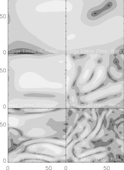
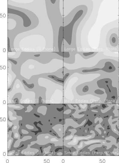
Figure 11: Anisotropy as a function of scale. (Left) Alfven mode velocity show scale-dependent anisotropy. (Right) Fast mode velocity show isotropy. Only part of the data cube is shown. Lighter tones are for larger $|{\bf v}|$. Magnetic field show similar behaviors.

References

- Andrews et al. (2001) Andrews, S. M., Meyer, D. M., & Lauroesch, J. T. 2001 ApJ, 552, L73
- Armstrong et al. (2001) Armstrong, J. W., Rickett, B. J., & Spangler, S. R. 1995, ApJ, 443, 209
- Batchelor (1950) Batchelor, G. K. 1950, Proc. Roy. Soc. Lond., A201, 405
- Batchelor (1959) Batchelor, G. K. 1959, J. Fluid Mech., 5, 113
- Beck (2002) Beck, R. 2002, preprint (astro-ph/0212288)
- Bertoglio et al. (2001) Bertoglio, J.-P., Bataille, F., & Marion, J.-D. 2001, Phys. Fluids, 13, 290
- Boldyrev (2002) Boldyrev, S. 2002, ApJ, 569, 841
- Boldyrev et al. (2002a) Boldyrev, S., Nordlund, Å., & Padoan P. 2002a, ApJ, 573, 678
- Boldyrev et al. (2002b) Boldyrev, S., Nordlund, Å., & Padoan P. 2002b, Phys. Rev. Lett. 89, 031102
- Brandenburg et al. (1996) Brandenburg, A., Jennings, R., Nordlund, A., Rieutord, M., Stein, R., & Tuominen, I. 1996, J. Fluid Mech., 306, 325
- Chandran (2000) Chandran, B. 2001, Phys. Rev. Lett., 85(22), 4656
- Cho & Lazarian (2002a) Cho, J., Lazarian, A. 2002a, Phy. Rev. Lett., 88, 245001 (CL02)
- Cho & Lazarian (2002b) Cho, J., Lazarian, A. 2002b, ApJ, 575, L63
- Cho et al. (2002a) Cho, J., Lazarian, A., & Vishniac, E. 2002a, ApJ, 564, 291 (CLV02a)
- Cho et al. (2002b) Cho, J., Lazarian, A., & Vishniac, E. 2002b, ApJ, 566, L49 (CLV02b)
- Cho et al. (2003) Cho, J., Lazarian, A., Honein, A., Knaepen, B., Kassinos, S., & Moin, P. 2003, ApJ, 589, L77
- Cho et al. (2003a) Cho, J., Lazarian, A., & Vishniac, E. 2003a, in Turbulence and Magnetic Fields in Astrophysics, eds. E. Falgarone & T. Passot (Springer LNP), p56 (astro-ph/0205286) (CLV03a)
- Cho et al. (2003b) Cho, J., Lazarian, A., & Vishniac, E. 2003b, ApJ, accepted (astro-ph/0305212)
- Cho & Vishniac (2000b) Cho, J. & Vishniac, E. 2000b, ApJ, 539, 273
- Cho & Vishniac (2000a) Cho, J. & Vishniac, E. 2000a, ApJ, 538, 217
- Del Zanna, Velli, & Londrillo (2001) Del Zanna, L., Velli, M., & Londrillo, P. 2001, A&A, 367, 705
- Deshpande (2000) Deshpande, A. A. 2000, MNRAS, 317, 199
- Deshpande, Dwarakanath & Goss (2000) Deshpande, A. A., Dwarakanath, K. S., & Goss, W. M. 2000, ApJ, 543, 227
- Dieter, Welch & Romney (1976) Dieter,N. H., Welch, W. J., & Romney, J. D. 1976, ApJ, 206, L113
- Draine & Lazarian (1999) Draine, B. T. & Lazarian, A. 1999, ApJ, 512, 740
- Faison & Goss (2001) Faison, M. D. & Goss, W. M. 2001, AJ, 121, 2706
- Goldreich & Sridhar (1995) Goldreich, P. & Sridhar, S. 1995, ApJ, 438, 763
- Goldreich & Sridhar (1997) Goldreich, P. & Sridhar, S. 1997, ApJ, 485, 680
- Heiles (1997) Heiles, C. 1997, ApJ, 481, 193
- Higdon (1984) Higdon, J. C. 1984, ApJ, 285, 109
- Jiang & Wu (1999) Jiang, G. & Wu, C. 1999, J. Comp. Phys., 150, 561
- Kida et al. (1991) Kida, S., Yanase, S., & Mizushima, J. 1991, Phys. Fluids A, 3, 457
- Kinney et al. (2000) Kinney, R. M., Chandran, B., Cowley, S., & McWilliams, J. C. 2000, ApJ, 545, 907
- Kolmogorov (1941) Kolmogorov, A. 1941, Dokl. Akad. Nauk SSSR, 31, 538
- Kulsrud & Anderson (1992) Kulsrud, R. & Anderson, S. 1992, ApJ, 396, 606
- Lazarian et al. (2002) Lazarian, A., Cho, J., & Yan, H. 2002, preprint (astro-ph/0211031)
- Lazarian & Esquivel (2003) Lazarian, A. & Esquivel, E. 2003, ApJ, accepted (astro-ph/0304007)
- Lazarian et al. (2003) Lazarian, A., Petrosian, V., Yan, H., & Cho, J. 2003, in press (astro-ph/0301181)
- Lazarian & Pogosyan (2000) Lazarian, A. & Pogosyan, D. 2000, ApJ, 537, 720
- Lazarian & Vishniac (1999) Lazarian, A. & Vishniac, E. T. 1999, ApJ, 517, 700
- Lazarian & Vishniac (2000) Lazarian, A. & Vishniac, E. T. 2000, Rev. Mex. A&A, 9, 55
- Lazarian, Vishniac & Cho (2003) Lazarian, A. & Vishniac, E. T., & Cho, J. 2003, ApJ, submitted
- Lazarian & Yan (2002) Lazarian, A. & Yan, H. 2002, ApJ, 566, L105
- Leamon et al. (1998) Leamon, R. J., Smith, C. W., Ness, N. F., Matthaeus, W. H., & Wong, H. 1998, J. Geophys Res., 103, 4775
- Lesieur (1990) Lesieur, M. 1990, Turbulence In Fluids (Dordrecht: Kluwer)
- Lithwick & Goldreich (2001) Lithwick, Y. & Goldreich, P. 2001, ApJ, 562, 279
- Liu & Osher (1998) Liu, X.& Osher, S. 1988, J. Comp. Phys., 141, 1
- L’vov, L’vov, & Pomyalov (2000) L’vov, V. S. & L’vov, Y. V., & Pomyalov, A. 2000, Phys. Rev. E, 61, 2586
- McKee (1999) McKee, C. F. 1999, in The Origin of Stars and Planetary Systems, ed. by J. L. Charles, D. K. Nikolaos (Dordrecht: Kluwer, 1999) p.29
- Mac Low et al. (1998) Mac Low, M.-M., Klessen, R., Burkert, A., & Smith, M. 1998, Phy. Rev. Lett., 80, 2754
- Maron & Goldreich (2001) Maron, J. & Goldreich, P. 2001, ApJ, 554, 1175
- Marscher et al. (1993) Marscher, A. P., Moore, E. M., & Bania, T. M. 1993, ApJ, 419, L101
- Matthaeus & Brown (1988) Matthaeus, W. H. & Brown, M. R. 1988, Phys. Fluids, 31(12), 3634
- Matthaeus et al. (1996) Matthaeus, W. H., Ghosh, S., Oughton, S., & Roberts, D. A. 1996, J. Geophysical Res., 101(A4), 7619
- Matthaeus et al. (1983) Matthaeus, W. H., Goldstein, M. L., Montgomery, D. C. 1983, Phys. Rev. Lett., 51, 1484
- Meyer & Blades (1996) Meyer, D. M. & Blades, J. C. 1996, ApJ, 464, L179
- (57) A. S. Monin, A. A. Yaglom: Statistical Fluid Mechanics: Mechanics of Turbulence, Vol. 2 (Cambridge: MIT Press, 1975)
- Myers & Lazarian (1998) Myers, P. & Lazarian, A. 1998m ApJ, 507, 157
- Müller & Biskamp (2000) Müller, W.-C. & Biskamp, D. 2000, Phys. Rev. Lett., 84(3), 475
- Padoan & Nordlund (1999) Padoan, P. & Nordlund, A. 1999, ApJ, 526, 279
- Passot & Vazquez-Semadeni (2003) Passot, T. & Vazquez-Semadeni, E. 2003, A&A, 398, 845
- Politano & Pouquet (1995) Politano, H. & Pouquet, A. 1995, Phy. Rev. E, 52, 636
- Reynolds (1988) Reynolds, R. J. 1988, ApJ, 333, 341
- Schekochihin et al. (2002) Schekochihin, A., Maron, J., Cowley, S., & McWilliams, J. 2002, ApJ, 576, 806
- Schlickeiser & Miller (1998) Schlickeiser, A. & Miller, J. A. 1998, ApJ, 492, 352
- She & Leveque (1994) She, Z. & Leveque, E. 1994, Phy. Rev. Lett. 72, 336
- Shebalin et al. (1983) Shebalin, J. V., Matthaeus, W. H., & Montgomery, D. C. 1983, J. Plasma Phys., 29, 525
- Spangler (1991) Spangler,S.R. 1991, ApJ, 376, 540
- Spangler (1999) Spangler,S.R. 1999, ApJ, 522, 879
- Stanimirovic & Lazarian (2001) Stanimirovic, S. & Lazarian, A. 2001, ApJ, 551, L53
- Stone, Ostriker, & Gammie (1998) Stone, J., Ostriker, E., & Gammie, C. 1998, ApJ, 508, L99
- Tafalla et al. (1998) Tafalla, M., Mardones, D., Myers,P., Caselli, P., Bachiller, R., & Benson, B. 1998, ApJ, 504, 900
- Thompson (1962) Thompson, W, B. 1962, An Introduction to Plasma Physics, (Pergamon Press)
- Vazquez-Semadeni (2000) Vazquez-Semadeni, E. 2000, in Advanced Series in Astrophysics and Cosmology, Vol. 10, eds. V. Gurzadyan & R. Ruffini (World Scientific), p.379
- Vazquez-Semadeni et al. (2000) Vazquez-Semadeni, E., Ostriker, E.C., Passot, T., Gammie, C.F., & Stone, J.M. 2000, in Protostars and Planets IV, eds. V. Mannings et al. (Tucson: University of Arisona Press), p.3
- Yan & Lazarian (2002) Yan, H. & Lazarian, H. 2002, Phy. Rev. Lett., 89, 281102
- Yan & Lazarian (2003) Yan, H. & Lazarian, H. 2003a, ApJ, accepted (astro-ph/0301007)
- Yan & Lazarian (2003) Yan, H. & Lazarian, H. 2003b, ApJ, submitted
- Zakharov (1967) Zakharov, V. E. 1967, Sov. Phys. JETP, 24, 455
- Zakharov & Sagdeev (1970) Zakharov, V. E. & Sagdeev, A. 1970, Sov. Phys. Dokl. 15, 439
- Zank & Matthaeus (1993) Zank, G. P. & Matthaeus, W. H. 1993, Phys. Fluids A, 5(1), 257