Evolution of the X-ray spectrum in the flare model
of Active Galactic Nuclei

Nayakshin & Kazanas (2002) have considered the time-dependent illumination of an accretion disc in Active Galactic Nuclei, in the lamppost model, where it is assumed that an X-ray source illuminates the whole inner-disc region in a relatively steady way. We extend their study to the flare model, which postulates the release of a large X-ray flux above a small region of the accretion disc. A fundamental difference to the lamppost model is that the region of the disc below the flare is not illuminated before the onset of the flare. After the onset, the temperature and the ionization state of the irradiated skin respond immediately to the increase of the continuum, but pressure equilibrium is achieved later. A few typical test models show that the reflected spectrum that follows immediately the increase in continuum flux should always display the characteristics of a highly illuminated but dense gas, i.e. very intense X-ray emission lines and ionization edges in the soft X-ray range. The behaviour of the iron line is however different in the case of a “moderate” and a “strong” flare: for a moderate flare, the spectrum displays a neutral component of the Fe K$\alpha$ line at 6.4 keV, gradually leading to more highly ionized lines. For a strong flare, the lines are already emitted by FeXXV (around 6.7 keV) after the onset, and are very intense, with an equivalent width of several hundreds eV. A strong flare is also characterized by a steep soft X-ray spectrum. The variation timescale in the flare model is likely smaller than in the lamppost model, due to the smaller dimension of the emission region, so the timescale for pressure equilibrium is long compared to the duration of a flare. It is therefore highly probable that several flares contribute at the same time to the luminosity. We find that the observed correlations between $R$, $\Gamma$, and the X-ray flux are well accounted for by a combination of flares having not achieved pressure equilibrium, also strongly suggesting that the observed spectrum is always dominated by regions in non-pressure equilibrium, typical of the onset of the flares. Finally, a flare being confined to a small region of the disc, the spectral lines should be narrow (except for a weak Compton broadening) and Doppler shifted, as stressed by Nayakshin & Kazanas (2001). All these features should constitute specific variable signatures of the flare model, distinguishing it from the lamppost model. It is however difficult, on the basis of the present observations and models, to conclude in favor of one of the hypothese.

1 Introduction

The model of “irradiated accretion disc” is now widely accepted as an explanation for the presence in the X-ray spectrum of Active Galactic Nuclei (AGN) of a Fe K$\alpha$ line and an X-ray hump (Pounds et al. 1990), and for the absence of time delay (or for the very short delay) between the variations of the optical and UV continuum fluxes (Collin-Souffrin 1991, Clavel et al. 1992). Both phenomena are most likely produced by an X-ray flux irradiating a cold medium (the accretion disc?), which leads to a signature as reprocessed radiation in the UV range, and to a Fe K$\alpha$ line and a Compton reflection hump in the X-ray range.

Three different models have been proposed to account for these properties: an X-ray source (whose origin is unknown) at a relatively high altitude above the disc, illuminating a large central region (the “lamppost”), a hot corona completely covering a cold disc (Haardt & Maraschi 1991, 1993), and finally a “patchy corona” (Haardt et al. 1994) partially covering the disc. This last model is often preferred for various reasons: the shape of the reflected continuum, the correlation between the Fe K$\alpha$ and the continuum, the absence or weakness of the helium- and hydrogen-like Fe lines (cf. Nayakshin 2000, Nayakshin & Kallman 2001), the fact that it allows us to account for the large UV over X observed luminosity ratio (cf. Walter et al. 1994). It is called the “magnetic flare” model, as it refers to magnetic loops reconnecting and suddenly releasing their energy as X-ray photons on a small portion of the disc.

There is presently no clear consensus concerning the physics of the flare, which is generally considered to be analogous to the sun. In particular, the height of a flare above the disc, its luminosity and its compactness are free parameters in addition to others that can be chosen in order to fit the observed variational and spectral properties of the objects. Poutanen & Fabian (1999) and Merloni & Fabian (2001) have proposed a model accounting for the spectral variability of accreting black holes (it is scaled for galactic sources, but it applies to AGN as well). Many simultaneous flares are required to account for the observed luminosity of an AGN. To avoid the smearing of strong luminosity variations, they propose that the amplitude of variability can be explained if these flares are triggered in a chain reaction. Each flare produces an “avalanche” of neighbouring flares, whose duration and amplitude determine the timing properties. In particular, the distribution of size and luminosity of the avalanches accounts for the shape of the power spectrum density, which gives the power as a function of the Fourier frequency (PSD, see also Zycki 2002). The most powerful avalanches have the largest size (corresponding to the largest time scales), and they correspond to the “break” and the red branch of the PSD (cf. below). In this model, the height of a magnetic loop increases during the avalanche, increasing the number of UV photons available for the cooling of the corona and causing the observed softening of the X-ray spectrum. It should be at least one order of magnitude larger than the pressure scale height of the disc. Consequently an avalanche can illuminate a relatively large fraction of the inner disc (since the radius of the illuminated region is of the order of the height of the source). Nayakshin & Kazanas (2001) argue on the contrary that the height of a flare should be of the order of the scale height of the disc, and that an avalanche of flares should illuminate only a very small fraction of the disc. In both cases the total number of simultaneous powerful avalanches is small, so that the total area illuminated by them is small compared to the disc area. This is a fundamental issue as it implies that the region of the disc located under an avalanche was not illuminated before the onset of the avalanche.

Our aim in this paper is to study the implication of this model, in particular on the soft X-ray spectrum and on the Fe lines. Note that in the following we will use the word “flare”, even if it is actually an avalanche.

Several recent results concerning time variations of the Fe lines are very intriguing in the context of irradiated discs. The expectation would be that the Fe lines respond to variations of the X-ray continuum flux in a simple way, in the same way as the broad optical-UV lines respond to the UV-X continuum flux. This is far from being the case, and the behaviour of the lines is actually very complex. The interpretations of the results are sometimes even contradictory, for instance for MCG -6-30-15 (Lee et al. 1999, Vaughan & Edelson 2001), where it is not clear whether the line flux stays constant, while the continuum varies. Another example is Mkn 841, where a rapid (less than 15 hours) and strong (a factor two) variation of the Fe K$\alpha$ line is related only to a weak variation (less than 20 $\%$) of the X-ray continuum (Petrucci et al. 2002).

Moreover the variations of the optical/UV continuum, which are generally assumed to be induced by variations of the X-ray flux and should therefore follow them after a short time delay if they are emitted by the accretion disc (Rokaki et al. 1993, Kazanas & Nayakshin 2001), do not obey a simple relationship with the X-ray light curves. For instance in NGC 7469, the UV flux leads the 2-10 keV flux in the peaks of luminosity (Nandra et al. 1998) while the 2-10 keV flux leads the UV flux during the minima of luminosity. However this effect can be an artefact due to the limited range of energy considered: since the X-ray spectrum becomes softer when the UV flux is large, the X-ray flux might be reprocessed below 2 keV. In NGC 3516 there is no clear correlation between the UV and the X-ray flux (Edelson et al. 2000).

It is clear that the response of the irradiated medium is not simply the consequence of the variation of the ionization state and of the thickness of the “hot skin” of the disc irradiated by a variable X-ray flux, as discussed either for a constant density medium or for a medium in hydrostatic equilibrium (Zycki & Różańska 2001). A most interesting idea stressed for the first time by Nayakshin & Kazanas (2002, hereafter NK02) is that if the illuminating flux varies on short time scales, the Fe line flux should not be a function of the instantaneous illuminating spectrum. In response to a variation of the illuminating flux, the atmosphere of the accretion disc remains during a relatively long time, required for readjustment of the hydrostatic balance, in a non-equilibrium state.

In this paper we extend this idea, discussing the fate of a region of the disc illuminated by a flare, a case not considered by NK02, who limited their study to the “lamppost model”. To clarify the discussion, Fig. 1 shows our vision of the lamppost and the flare models.

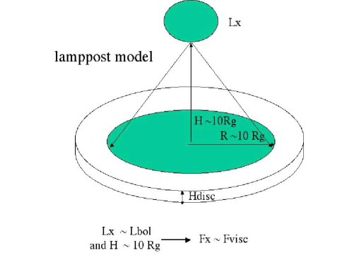
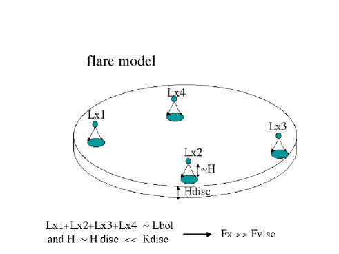
Figure 1: The lamppost and the flare models.

In both cases, the disc is illuminated by an X-ray source whose luminosity is equal to a fraction of the bolometric luminosity, located at a given height $H$ above the disc. The lamppost is located in the center (above the black hole), and its height is of the order of 10-20 $R_{G}$ ($R_{G}$ being the gravitational radius $GM/c^{2}$), while a flare is located at any radius, and its height above the disc is much smaller. Several flares can be shining at the same time. The dimension of the region illuminated by a source located above the disc is of the order of its height, and the flux on this region is of the order of $L/4\pi H^{2}$. For a flare, the flux is thus much larger than for a lamppost. It is also much larger than the viscous flux provided by the release of gravitational energy, which is maximum at a few $R_{G}$ and decreases as $R^{-3}$ (where $R$ is the distance to the center).

According to this discussion, we assume therefore that the flare model differs from the lamppost model in three respects:

• In the lamppost model, the disc is illuminated permanently. The illuminating flux can switch from a state $F_{X1}$ to a state $F_{X2}$, with $F_{X2}\sim$ a few $F_{X1}$, or inversely, but the illumination is always present. Therefore an irradiated layer, called the “hot skin”, always exists above the inner disc. However the hydrostatic equilibrium corresponding to the two states is different, and the hot skin as well as its spectrum will evolve slowly (cf. later) from one equilibrium state to the other. On the contrary, in the flare model, there is no illumination in the initial state (and in the final state, after the extinction of the flare), so the newly formed hot skin is much denser than an illuminated atmosphere (it does not exclude that another part of the disc is already illuminated, as we will discuss in Section 4).

• In the lamppost model, the disc is illuminated by a flux $F_{X}$ smaller than or of the order of the viscous flux $F_{d}$, while in the flare model, $F_{X}$ is much larger than $F_{d}$.

• In the lamppost model, the whole inner disc is illuminated, while in the flare model the illumination acts only on a small fraction of the disc.

In the following section, we recall the relevant time scales, and in Section 3 we give results corresponding to a few typical cases. Implications for the observations are discussed in Section 4.

2 Physical parameters

2.1 Time scales

When the X-ray flux varies, the illuminated medium responds with different characteristic times. Though they are recalled by NK02, we give them here in the context of the present study.

1. The radiation transfer time, $t_{rt}$. In a completely ionized medium, $t_{rt}=\tau_{es}(1+\tau_{es})/(\sigma_{T}cn)$, where $\tau_{es}$ is the Thomson thickness of the reflecting medium, $\sigma_{T}$ is the Thomson cross section, and $n$ is the electron density (note that resonance line scattering can also play a role, cf. below). Since X-ray photons are absorbed in a few Thomson units, the optical thickness of the hot skin is smaller than or of the order of unity, and therefore $t_{rt}\leq 100n_{12}^{-1}$ s, where $n_{12}$ is the density expressed in 10¹² cm^-3. We will see that the average density at the onset of the flare is probably larger than 10¹² cm^-3. So $t_{rt}$ is small, and the whole atmosphere receives the new flux quasi-simultaneously.

2. The time for readjustment of the ionization equilibrium, which is the longer of the ionization time, $t_{ion}$, and the recombination time, $t_{rec}$. One has $t_{ion}\sim<h\nu>/(F_{X}\sigma_{ion})$, where $<h\nu>$ is the mean energy of the ionizing photons, and $\sigma_{ion}$ is the ionization cross-section. For the physical conditions holding near the surface of the accretion disc, $t_{ion}\sim 10^{-7}F_{16}^{-1}$ s, where the flux is expressed in 10¹⁶ ergs cm^-2 s^-1, a typical value for $F_{X}$ during a flare (cf. Nayakshin et al. 2000, Ballantyne & Fabian 2001, and below). $t_{rec}\sim 1/(n\alpha_{rec})\sim 10n_{12}^{-1}$ s, where $\alpha_{rec}$ is the recombination coefficient of the ion under consideration. So again these times are short, and one can consider that the medium readjusts instantaneously to the new conditions.

3. The time for thermal equilibrium, $t_{therm}$, i.e. the time required to radiate the energy of the medium, $nkT/(n^{2}\Lambda)$, where $\Lambda$ is the cooling function. At the onset of a flare, $\Lambda$ is dominated by atomic processes and is of the order of 10^-23 erg cm⁺³ s^-1. This gives $t_{therm}\sim 10T_{6}n_{12}^{-1}\Lambda_{23}^{-1}$ s, again a small value .

4. The time for readjustment of the hydrostatic equilibrium (the dynamical time). Actually this time is of the order of that necessary to create the hot skin, $t_{dyn}=H/c_{s}$, where $H$ is the scale height of the atmosphere (after hydrostatic equilibrium), and $c_{s}$ is the sound velocity in the hot skin (after thermal equilibrium). Indeed the hydrostatic equilibrium of the disc itself is almost not changed by the illumination if $F_{X}/F_{d}\ll\tau_{disc}$ (except possibly close to the surface), where $\tau_{disc}$ is the optical thickness between the surface and the equatorial plane (cf. Hubeny 1990, Huré et al. 1994), a condition easily fulfilled as the disc is optically very thick for typical accretion rates in quasars and Seyfert galaxies. For a Thomson thickness of the atmosphere of order of unity, $t_{dyn}\sim 10^{5}T_{6}^{-1/2}n_{12}^{-1}$ s, if one assumes that the readjustement takes place at the sound speed. It is possible that shock waves with a relatively high Mach number contribute to this readjustment, so the dynamical time could be smaller. Even in this case, $t_{dyn}$ would be much larger than the previous “microscopic” time scales.

Figure 2: Temperature and density versus $\tau_{es}$ for model H1, before (state 1), after the onset of the flare (state 2), and after pressure equilibrium is reached (state 3); dotted line: temperature; solid line: density. We recall that state 2 is reached at a time $t_{grow}\sim 10^{3}$ s after the beginning of the flare, while state 3 is achieved after a much longer time, $t_{dyn}\sim 10^{5}$ s.

The onset of a flare is not instantaneous, and all these times should be compared to the variability time scale of the illuminating continuum. Three time scales are of interest in this context.

First, one has to take into account the “growing” time of a flare (or equivalently the “fading” time) as seen from the underlying disc, $t_{grow}$. It is probably of the order of the vertical extension of an individual flare divided by the Alfven velocity. One can assume that the dimension of a magnetic loop is of the order of the scale height of the disc (Nayakshin & Kazanas 2001). In the standard model of accretion discs (Shakura & Sunayev 1973) where the inner regions are dominated by radiation pressure and Thomson opacity, this scale height is roughly equal to 10${}^{13}M_{8}\dot{m}_{-1}$ cm, where $\dot{m}_{-1}$ is the bolometric to Eddington luminosity ratio in units 0.1, and $M_{8}$ is the black hole mass in 10⁸M_⊙. Thus $t_{grow}$ should be of the order of 10³ s.

Second, one should consider the time scale corresponding to the observed increase of the X-ray continuum, $t_{fl}$, i.e. to the onset of the whole avanlanche. It is difficult to predict theoretically, but one knows that the PSD extends from 10^-5 to 10^-2 Hz, and consists of two power laws and a break at $\sim 3\ 10^{-4}$ Hz, which should correspond to the largest and most powerful active regions. Accordingly, $t_{fl}$ is larger than, or of the order of $t_{grow}$, and smaller than the dynamical time. One deduces also that the radius $R_{fl}$ of powerful flares is smaller than 10¹⁴ cm. It is therefore smaller than the radius of the inner accretion disc giving the bulk of the viscous dissipation, $\sim 20R_{G}=3\ 10^{14}M_{8}$ cm. Note that it is in agreement with the conclusion of Nayakshin & Kazanas (2001) based on a different argument.

The third timescale is the whole duration of a flare, for which we have no real indication, and which could well be as large as 10⁵ s (the largest time given by the PDS).

To summarize, one has:

$$t_{microscopic}\ll t_{grow}\sim 10^{3}\ {\rm s}\leq t_{fl}\ll t_{dyn}\sim 10^{5}\ {\rm s}.$$ (1)

Compared with the sampling time of an observation, the onset of the flare can thus be observed. The temperature and the ionization equilibrium respond immediately to an increase of flux, but the density structure stays unchanged. The adjustement in density (i.e. in pressure) is much longer, and might not be achieved before the flare ends, or before another flare has begun. So it is likely that the observed spectrum corresponds to a mixture of spectra in different non-equilibrium phases.

An important point to notice is the difference in timescales between the lamppost and the flare models, simply due to the larger size of the illuminated region in the lamppost model: while a typical time for the onset of a flare should be $10^{3}$ s, it should be at least one order of magnitude larger for the lamppost model. We recall that all these times refer to a black hole mass of 10⁸M_⊙.

2.2 Fluxes

Figure 3: Fractional ionization of oxygen and iron for model H1.

The flare model is characterized by the fact that most of the disc receives a very small illumination, whereas one region is suddenly illuminated by an X-ray flux $F_{X}$ much larger than the underlying viscous flux $F_{d}$. So one can neglect the incident flux before the flare.

To account for the observed X-ray variability, a flare should have a luminosity comparable to the average X-ray luminosity, which is itself a fraction $f$ of the bolometric luminosity (typically $f\sim 10\%$). It means that the illuminating flux in the region covered by the flare should be of the order of:

$$F_{X}\sim 10^{17}f_{-1}\dot{m}_{-1}M_{8}^{-1}r_{fl}^{-2}\ \ {\rm erg\ cm}^{-2}{\rm s}^{-1}$$ (2)

where $f_{-1}$ is expressed in units of 0.1, and $r_{fl}$ is the size of the flaring region expressed in $R_{G}$. Since the model implies that this size is small compared to the radius of the disc corresponding to the bulk of the “viscous” luminosity, say 20$R_{G}$, the illuminating flux is larger than the viscous flux

$$F_{d}\sim 10^{15}\eta_{-1}^{-1}\dot{m}_{-1}M_{8}^{-1}\left({R_{ill}\over 20R_{G}}\right)^{-3}\ \ {\rm erg\ cm}^{-2}{\rm s}^{-1}$$ (3)

where $\eta_{-1}$ is the efficiency of mass-energy conversion in units 0.1 and $R_{ill}$ is the radius of the illuminated region. Thus after the onset of the flare, one can neglect the viscous flux.

3 Test models

It is out of the scope of this paper to solve a real time-dependent problem, which would be very difficult to handle, as it would imply a dynamical study accounting for shocks and winds. We only want to show what kind of spectral features should characterize the flare model, when an important variation of the X-ray flux is detected (say, a few tens of $\%$). We will assume that at a time t=0, the disc is irradiated by a flux larger than the viscous one, which then remains constant. The thermal and ionization equilibria respond to the variation of the illuminating flux only in a few tens seconds. Then the atmosphere begins to expand slowly under the effect of the radiation plus gas pressure. If the flare lasts for more than, say, one day, hydrostatic equilibrium can be achieved. We will simply show the difference of spectra a short time after the flare, and after hydrostatic equilibrium is reached. To this aim we use several test-models.

3.1 Standard disc

The first model is a standard irradiated $\alpha$-disc in hydrostatic equilibrium in the gravitational field of the central black hole. The method for solving the transfer and the vertical structure of the disc is described in Różańska et al. (2002). Briefly summarized, two computations are coupled. In the inner layers, the vertical structure is computed according to Różańska et al. (1999); the radiative transfer is treated in the diffusion approximation with convective transport included; the viscous energy dissipation is given by the local $\alpha$-viscosity description, with the viscous energy generation proportional to the total pressure. In the superficial layers ($\tau_{es}\leq 10$), the transfer is solved with the photoionization-transfer code Titan described in Dumont et al. (2000) and updated by Coupé et al. (2003) to include improved atomic data and a larger number of transitions. Comptonization is taken into account above 1 keV through the coupling with a Monte Carlo code, NOAR, also described in Dumont et al. (2000). The vertical temperature and the density profiles are determined according to hydrostatic equilibrium, both in the disc and in the hot skin. When multiple solutions arise in the atmosphere, the “hot solution” is chosen (actually this choice has no influence on the spectrum for the high flux considered here, cf. Coupé et al. 2002).

The test model is an accretion disc around a Schwarzschild black hole of mass $M=10^{8}$ M_⊙, with an accretion rate $\dot{m}=L/L_{Edd}=0.001$ and a viscosity parameter $\alpha=0.1$ (model H1). Before the time $t=0$, the disc is not illuminated. After the time $t=0$, the disc is illuminated by a flux equal to 10${}^{15}\ {\rm erg\ cm}^{-2}{\rm s}^{-1}$. We assume that the flare takes place at a radius $R$ equal to 18$R_{G}$, corresponding to a viscous flux of 7 $10^{12}\ {\rm erg\ cm}^{-2}{\rm s}^{-1}$. The spectral distribution of the incident continuum is a power-law with an energy index $0.9$, extending from 1 eV up to 100 keV. This model will be discussed in detail by Różańska et al. in a paper in preparation, mainly aimed at comparing low and high illumination of the disc, and their results with those obtained by other groups. Note that the model can correspond to a different set of values of $M$, $\dot{m}$, and $R$, as the main parameters which matter in this problem are $F_{X}$, $F_{X}/F_{d}$, here equal to 140, and the gravity parameter $A$ defined by Nayakshin et al. (2000), here equal to 0.023 just after the flare, and to 0.34 when hydrostatic equilibrium is achieved.

Fig. 2 displays the vertical distribution of density and of temperature in the atmosphere, before the onset of the flare (state 1) and after a time $t_{grow}$ (state 2). In state 1, the disc atmosphere is cold and relatively dense ($T\sim 10^{4}$ K and $n\sim 10^{14}$ cm^-3 at $\tau_{es}=1$). In state 2, the density profile is not changed, but thermal and ionization equilibria are achieved and $T$ reaches 10⁷ K in a skin of optical thickness $\tau_{es}\sim 0.3$. After the much longer time $t_{{dyn}}$, hydrostatic equilibrium is achieved (state 3), the density averaged over the hot skin is smaller ($n\sim 10^{12}$ cm^-3), and the hot skin extends deeper into the disc. It is interesting to note that the temperature profile is more abrupt when pressure equilibrium is achieved, leading in particular to the disappearance of intermediate ionization states. This is well known and due to the thermal instability generally present in a slab having an imposed pressure (Ko & Kallman 1994).

Fig. 3 shows the comparison between the fractional ionization of oxygen and iron in states 2 and 3. One sees clearly that in state 2 the layer contributing to the bulk of the reflection spectrum ($\tau_{es}\sim 0.1$ to 1) is dominated by intermediate species of iron and by OVII and OVIII ions, while in state 3 it is dominated by fully ionized iron and oxygen.

Figure 4: Computed spectrum for states 2 and 3 of model H1. The top figure gives the ratio of the reflected to the incident spectrum, and the two bottom figures give the sum of the two components (i.e. the observed spectrum) in two spectral ranges. Some lines and edges are identified (lines: above the spectrum; edges: below the spectrum). The spectra are displayed with a spectral resolution of 44.

This explains the behaviour of the reflected and observed spectra for states 2 and 3, shown in Fig. 4 (we recall that in state 1 there is no reflection at all). The top figure gives the ratio of the reflected to the incident spectrum, and the two bottom figures show the reflected plus incident spectrum in two spectral bands, to perform a direct comparison with the observations .

Let us compare the spectra of the two states in the different spectral bands:

- In the keV range

In state 2 the gas is not highly ionized, so the spectrum displays a Fe K$\alpha$ line at 6.4 keV, which appears as an intense shoulder in the line profile, itself peaking at 6.7 keV, and dominated by the FeXXV line. H-like iron is very weak, as is the ionization edge at 10 keV. In state 3, the reflecting layer is thicker, the reflected continuum is more intense (in other words the albedo is larger), the 6.4 keV line has disappeared, and the FeXXVI Ly$\alpha$ line at 6.9 keV has appeared, as well as an intense ionization edge in absorption at 10 keV. Note also that the iron line displays intense Comptonized wings, in particular on the red side, which are completely absent in state 2.

- In the soft X-ray range

In state 2, the spectrum displays very intense lines and ionization edges in emission, which are much weaker in state 3. In this last state, the soft X-ray lines should be partly smeared out by Comptonization, which is not taken into account in this energy range with our code, so the lines should be even less visible .

It is interesting to note that the continuum is curved and does not look like a power-law, even in a small energy range. In particular its shape in the 2-10 keV range varies from state 2 to state 3, and could well mimic the variation of an extended relativistic red wing.

The presence of the neutral iron line after the onset of the flare is caused by the specific model chosen here, where the illuminating flux is not very high. In the case of a larger flux, the illuminated skin could be highly ionized immediately after the onset of the flare, as we will see in the next section. If the illuminating flux reaches a very high local value, the hot skin can become completely ionized and the lines and edges can decrease and even disappear completely (cf. Nayakshin & Kallman 2001).

3.2 Medium in pressure equilibrium

Figure 5: Gas and radiative pressure for model P2; solid line: gas pressure after the onset of the flare, and before pressure equilibrium is reached (state 2); dotted line: gas, radiative, and total pressure after pressure equilibrium is reached (state 3): the total pressure is constant and equal to the gas pressure at the surface in state 2.

Figure 6: Temperature and density versus $\tau_{es}$ for models P1 and P2; dotted line: temperature; solid line: density.

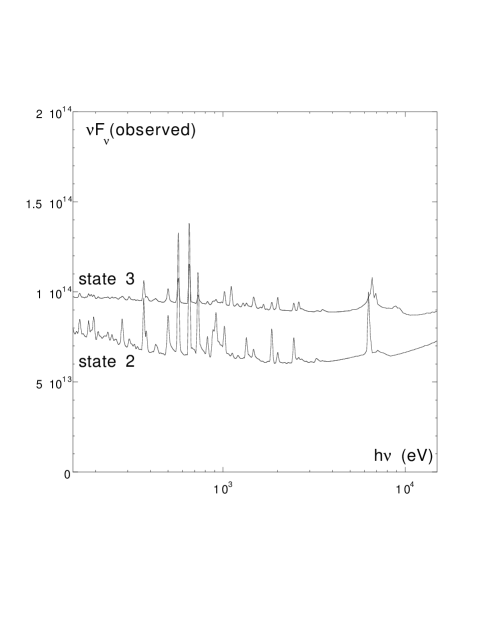
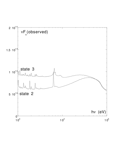
Figure 7: Computed spectrum for model P1 (moderate flare), after onset of the flare (state 2) and after pressure equilibrium is reached (state 3). The top figure gives the ratio of the reflected to the incident spectrum, and the two bottom figures give the sum of the two components (i.e. the observed spectrum) in two different spectral ranges. The spectra are displayed with a spectral resolution of 44.

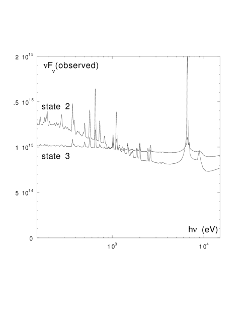
Figure 8: Same as 7 for model P2 (strong flare).

We have performed two other tests, replacing the achievement of hydrostatic equilibrium by the achievement of a constant total pressure. First it is not obvious that the only explanation for the properties of AGN is the “standard irradiated disc” model in hydrostatic equilibrium, and other models have been proposed: very dense cloudlets in a spherical optically thin accretion flow (Rees 1987, Kuncic et al. 1997), or quasi-spherical distribution of more dilute clouds (Collin-Souffrin et al. 1996). Second, the disc model is strongly parameter-dependent. Its structure depends on the value of the viscosity parameter $\alpha$, on the vertical distribution of energy deposition, and even on the assumption made for the stress tensor (given by gas-pressure or by total pressure, or by a combination of both). None of these issues have yet been definitively established. Assuming that the illuminated medium tends to settle at a constant pressure avoids the model-dependency of the results, and it leads to a significant computational simplification. Moreover this condition is not very different from hydrostatic equilibrium. The geometrical thickness of the hot skin is at most equal to a few disc scale heights (cf. the appendix of Różańska et al. 2002). Thus the gravity does not vary much between the base of the atmosphere and the height corresponding to the bulk of the reflection (i.e. between $\tau_{es}$ = 0.01 and 1).

Note also that there is an argument favoring a non-zero gas pressure at the surface of the non-perturbed accretion disc. The magnetic loops supposed to give rise to the flare are most likely located in a hot corona. The presence of this corona, even very dilute and contributing negligibly to the X-ray emission, is felt by the disc as it exerts a gas pressure on the surface. The boundary condition is changed, and in particular the surface density is increased. For instance in the disc/corona model studied by Różańska et al. (2002), the density in the disc atmosphere is constant and of the order of $10^{15}$ cm^-3 in the whole atmosphere of the disc (defined by $\tau_{es}\leq 1$). So the density chosen in these test models ($10^{14}$ cm^-3) could well correspond to an atmosphere pressurized by a weak corona.

We have therefore used two models: model P1 corresponds to a modest flare, and model P2 to a strong flare. In both models we assume that the unperturbed medium is a slab of constant density $n=10^{14}$ cm^-3 and optical thickness $\tau_{es}=25$, illuminated after $t=0$ on one side by a flux which remains constant until pressure equilibrium is reached. The incident flux is $F_{X}=10^{15}\ {\rm erg\ cm}^{-2}{\rm s}^{-1}$ in model P1, $10^{16}\ {\rm erg\ cm}^{-2}{\rm s}^{-1}$ in model P2. The spectral distribution is a power law $F_{\nu}\propto\nu^{-1}$ from 0.1 eV to 100 keV (this spectral shape is chosen to allow comparison with the set of models already obtained in another context, cf. Coupé et al. 2003). The backside of the slab is illuminated by a blackbody of 30000K, to mimic viscous dissipation, as was done for instance by Ross & Fabian (1993). It has no influence on the reflected X-ray spectrum, since the corresponding viscous flux is much smaller than $F_{X}$. The total pressure of the final state is constant and equal to the gas pressure at the surface after the onset of the flare (cf. Figs. 5 and 6). This was assumed in order to mimic the situation of an accretion disk, where there is a high gas pressure underlying the hot skin which inhibits its expansion towards the back (actually there is a small mismatch in model P1, which has no consequence for the emission spectrum).

Fig. 6 displays the temperature and density profiles, at time $t_{grow}$ after the onset of the flare (state 2), and after a time $t_{dyn}$, when pressure equilibrium is achieved (state 3) (state 1 before the onset of the flare corresponds to a low temperature medium with almost no emission).

It is interesting to note that in the final equilibrium (state 3) the temperature profiles are almost the same for both models, as well as the optical thickness of the hot layer. This is due to the fact that the “ionization parameter” (radiative flux to gas density ratio at the surface) is similar in both models. However the density is about one order of magnitude larger for model P2 in the deep layers, where gas pressure dominates radiative pressure, since radiative pressure is one order of magnitude larger in the surface layers. The density on the illuminated side is not well determined, as gas pressure is completely negligible there. On the contrary, in the initial state 2, the optical thickness of the hot skin is almost one order of magnitude larger in model P2 than in model P1, as model P2 corresponds to a larger ionization parameter than model P1.

Note also that the temperature profile is smoother when pressure equilibrium is not achieved, as in the hydrostatic case.

Figs. 7 and 8 display the spectra for both models.

The spectrum of model P1 looks like that of model H1, as expected, at least for the reflected to incident ratio. The “observed” spectrum is slightly different, owing to the different spectral index of the incident continuum (the photon index $\Gamma$ is equal to 1.9 for model H1 and to 2 for models P1 and P2). The spectrum in state 2 is characterized by an intense Fe K$\alpha$ line at 6.4 keV, and a curvature of the continuum. When pressure equilibrium is achieved, the reflected continuum is flatter, more intense, and the lines correspond to more ionized species, as in state 3 of model H1.

Model P2 leads in state 2 to a very steep reflected spectrum in the soft X-ray range (i.e. the albedo is larger than unity below 1 keV and smaller above 1 keV), while the emission lines (for instance the iron lines) correspond to highly ionized species (FeXXV and FeXXVI). It is because there is a large intermediate zone contributing to the reflection spectrum where the temperature decreases smoothly from 10⁷ K to 10⁵ K. The spectrum in state 2 is also characterized by intense lines and edges in the soft X-ray range, but the iron line is dominated by FeXXV lines, and the 6.4 keV line is absent. In state 3, model P2 leads to a spectrum similar to model P1, owing to their similar temperature structure.

So we see that the structure and the spectrum are not very dependent on the power of the flare at pressure equilibrium. On the contrary, after the onset of the flare, for a strong flare the soft X-ray spectrum is steep and the - very intense - iron line is dominated by highly ionized species, while for a moderate flare the X-ray spectrum is relatively flat and the - weak - iron line is dominated by neutral K$\alpha$ lines at 6.4 keV. For instance the equivalent width of the iron complex is equal, in state 2, to 440 eV for model P2, and only to 104 eV for model P1, while the EWs are almost the same in state 3 (100 and 78 eV respectively).

It is interesting also to compare the spectra obtained in the hard X-ray and gamma-ray range. While Comptonization of the iron line is important in states 2 and 3 for the strong flare (model P2), it is negligible for state 2 of the moderate flare (model P1). In particular the moderate and the strong flare lead to a very different local iron line profile before pressure equilibrium is achieved.

Figure 9: Computed spectrum for states 1, 2 and 3 of combination 1 (cf. text for explanations). The figure gives the sum of the reflected + incident spectrum (i.e. the observed spectrum). The spectra are displayed with a spectral resolution of 44.

Figure 10: Same as Fig. 9 for combination 2.

Figure 11: Same as Fig. 9 for combination 3.

4 Discussion

4.1 Mixture of flares

More than one flare can be present at the same time. However there are certainly not many of them, otherwise the variations would be completely erased by the time delays and by the addition of many contributions. The observed spectrum should therefore be a mixture of a few flares in different states. Actually, since the flares are independent, the observed spectrum is simply the addition of these different spectra weighted by the luminosity of each flare.

Fig. 9 displays the observed spectrum for a combination of flares, assuming that all flares are similar to model H1 (combination 1). State 1 corresponds to the addition of two flares having reached their hydrostatic equilibrium: i.e. state 1 of combination 1 = the addition of two states 3 of model H1. A third flare begins to shine. After a time $t_{grow}$, the ensemble reaches state 2 of combination 1 that equals the addition of two states 3 of model H1, and one state 2 of model H1. Finally, after a time $t_{dyn}$ the third flare also reaches hydrostatic equilibrium; it is state 3 of combination 1 = the addition of three states 3 of model H1.

We see in Fig. 9 that the increase of the flux due to the new flare is linked to the appearence of lines in the soft X-ray range, and that of the Fe K$\alpha$ line at 6.4 keV, visible as a shoulder in the red wing of the line. These lines should slowly disappear as the disc reaches hydrostatic equilibrium below the flare.

Fig. 10 displays the observed spectrum for another combination of flares (combination 2). State 1 of combination 2 corresponds to the addition of ten flares similar to model H1, having reached their hydrostatic equilibrium (state 3 of model H1). A new flare begins to shine, but now it is a strong one, similar to model P2: i.e. state 2 of combination 2 = the addition of ten states 3 of model H1 and of one state 2 of model P2. Again, the increase of the flux is linked with the apparition of intense lines in the soft X-ray range, but contrary to the previous case, the iron line at the beginning of the flare is already due to highly ionized species. The intensities of all these lines decrease when hydrostatic equilibrium is reached.

Until now, we have only considered a simple change of flux during a flare, not accompanied by a change of the spectral shape. However there is growing observationnal evidence for a large number of Seyfert, that the X-ray spectrum softens as the 2-10 keV flux increases (Perola et al. 1986; Yaqoob et al. 1993; Lee et al. 1999; Lamer et al. 2000; Chiang et al 2000; Petrucci et al. 2000; Vaughan & Edelson 2001; Zdziarski & Grandi 2001; Georgantopoulos & Papadakis 2001). We have mentioned that Merloni & Fabian (2001) interpret this effect as being due to the development of an avalanche.

We have therefore also considered a third combination, which is the case of a flare beginning with a relatively hard spectrum ($\Gamma$=1.9). When the luminosity increases, the incident continuum softens, reaching $\Gamma$=2. The first flare has the same parameters as the moderate flare of model P1, except that the spectral index of the incident continuum is equal to 1.9. When thermal equilibrium, but not pressure equilibrium, is achieved, its spectrum is basically similar to state 2 of model P1, except that the slope of the continuum is harder. It corresponds to state 1 of combination 3. Then the luminosity doubles as the spectral index increases and the flare becomes similar to model P1: it is state 2 of combination 3, equal to the addition of two states 2 of model P1. State 3 of combination 3 corresponds to the achievement of pressure equilibrium and therefore to the addition of two states 3 of model P1. Fig. 11 displays the observed spectrum for combination 3. In the next section we will show the interest of this model, where the increase in luminosity is accompanied by a softening of the spectrum.

4.2 Comparison with the observations

4.2.1 Correlations between continuum parameters

A correlation between the amplitude of the reflection component $R$ ($R$ is normalized so that $R=1$ in the case of an isotropic source above an infinite reflecting plane) and the photon index $\Gamma$, has been found by Zdziarski et al. (1999) in a large sample of Ginga spectra of Seyfert galaxies. The measured $R$ tends to be larger in softer sources. This correlation is observed in different samples of sources as well as in the time evolution of individual sources. The $R$-$\Gamma$ correlation is also found in the BeppoSAX data (Matt 2001, and Perola et al. 2001), the BeppoSAX sample showing however a significantly different shape, with on average higher $R$ values at low $\Gamma$ and a flatter correlation. This correlation is still widely controversial, in particular regarding the uncertainties on the measurement of $R$. However no-one could prove that it is an artefact. The usual interpretation of the correlation invokes the feedback from reprocessed radiation emitted by the reflector itself. Very approximately, if such a correlation exists, one can represent it as $\delta R\propto 4\ \delta\Gamma$ for $\Gamma$ of the order of 2.

As mentioned previously, a correlation between $\Gamma$ and the X-ray flux is also observed in Seyfert galaxies. We note however that the fluxes used are generally restricted to a narrow energy band, usually 2-10 keV, and it is not clear if the total X-ray luminosity would follow the same correlation (Petrucci et al. 2000). One observes an increase of $\Gamma$ of 0.2 for an increase of the flux by a factor 2 (cf. the fit of the correlation $\Gamma$-Flux of MCG -6-30-15 of Merloni & Fabian 2001).

Figure 12: Correlation between $\Gamma$ and $F$(2-10keV) expected during a flare, and deduced from the fits of the spectra. See text for explanations.

Figure 13: Correlation between $R$ and $\Gamma$ expected during a flare, and deduced from the fits of the spectra. See text for explanations.

To see whether we can obtain these correlations with the flare model, we have analyzed our different spectra with xspec. For that purpose, we needed to create, from our simulations, standard pha and unit diagonal response matrix files using the task flx2xsp of ftools. We assumed error bars of 5% for each energy bin. We then fitted our spectra with the pexrav model of xspec which has 3 parameters, the photon index $\Gamma$, the reflection normalization $R$ and the high energy cut-off $E_{c}$. Our spectra being limited to the 0.1-70 keV energy band, we fixed $E_{c}$ at 400 keV for all fits (we have checked that, even if other values of $E_{c}$ could result in small changes of our best fit values and especially $R$, their relative trends between the different states, which is what we are interested in, is insensitive to the value of $E_{c}$). The fits have been made in two energy ranges, from 100 eV to 15 keV, and from 100 eV to 70 keV. The results for the two fits are in good agreement.

Fig. 12 shows the correlation between $\Gamma$ and $F$(2-10keV) computed with the different individual models (top figure) and the different combinations (bottom figure). It is clear that none of the individual models agrees with the observations, i.e. they do not show an increase of the spectral index correlated with an increase of the flux. On the contrary, some combinations account well for the correlation: combination 1, between states 2 and 3, combination 2, between states 1 and 2, i.e. during the onset of a flare superposed on several old flares, and combination 3, also between states 1 and 2, i.e. during the onset of a moderate flare, where it is assumed that the slope of the incident X-ray spectrum itself increases during the increase of luminosity. A likely explanation for the lack of agreement between the observations and the individual models could be that the flares do not last long enough for the atmosphere to achieve hydrostatic equilibrium, and that another flare begins before the atmosphere below the previous one has reached pressure equilibrium. In this case, the observed spectrum would be dominated by several flares in non-equilibrium states, and would display short-term variations (on $10^{3}-10^{4}$ s), similar to states 1 and 2 of combinations 2 and 3. This result suggests that the luminosity is always dominated by regions of the disc having not reached their pressure equilibrium.

Fig. 13 shows the correlation between $R$ and $\Gamma$. A correlation between the two parameters is visible on all the individual models and the combinations. It is similar to that observed by Zdziarski et al. (1999), even if our best fit values do not completely agree with that reported by these authors. This could be explained in part by the fact that our simulations suppose a simple power law up to 100 keV for the continuum while we fit our spectra assuming $E_{c}$=400 keV. It is not a critical point in our study however, since the presence of a remote reflector (a torus) far from the central engine, which has not been taken into account in our simulations, could easily reproduce the $R$-$\Gamma$ correlation reported in the literature (Malzac & Petrucci 2002).

4.2.2 Line spectrum

Nayakshin & Kazanas (2001) stressed that the lines emitted during a flare should be narrow, owing to the small dimension of the active region, and they should move in the frequency space according to the rotation of the disc. The shift in frequency would prevent one from distinguishing between a neutral and an ionized iron line if there is only one line. But if several ionization states are present, the frequency ratios would remain constant, and the frequency shift would constitute a specific signature of a flare.

The high sensitivity of the XMM-Newton satellite has recently permitted the detection of narrow and rapidly variable iron lines. Petrucci et al. (2002) report a highly variable iron line in Mkn 841, unresolved with the XMM-pn instrument, which disappears in about 15 hours. Turner et al. (2002) claim, also from XMM-pn observations, the presence of several variable narrow components within the profile of the iron $K_{\alpha}$ line in NGC 3516. The presence of a varying narrow line component in MCG -6-30-15 has also been detected by Lee et al. (2002) in Chandra HETGS observations. In the two latter cases, the line variability appeared to be related to changes in the continuum flux. The lines have been interpreted by the different authors as the narrow red or blue wings of relativistically broadened profiles. It thus agrees with the interpretation that magnetic flares, such as those studied here, may provide the source of enhanced continuum emission by illuminating small areas of the accretion flow. The flares have then to be produced near the central black hole to explain the relativistic broadening.

In the case of Mkn 841, there were apparently no or only small changes of the X-ray continuum when the iron line decreased or even disappeared. An interpretation which could be proposed is that the line observed during the first observation was due to a very strong flare still out of pressure equilibrium. When pressure equilibrium was achieved (which could have happened during the time between the two observations), the line became very weak, while the continuum did not increase more. This would be similar to our model P2, except that the flare would have to be even stronger. New observations are clearly needed to confirm the line variability in this source. We note however that it may also be produced by different processes (like the presence of a concave disc as proposed by Blackman 1999) which do not necessarily require variations of the continuum.

Concerning the soft X-ray spectrum, it is difficult presently to perform a detailed comparison with the existing spectra, such as that of MCG -6-30-15. This would require the presence of a warm absorber in addition to the disc itself, and to take into account Comptonization in the lines, which would smear the profiles, especially when pressure equilibrium is achieved. We intend to perform such computations in the near future.

5 Conclusion

We have made a preliminary study of the consequences of the flare model on the X-ray spectrum and on its time variations.

We have in particular stressed the importance of the transient state during which the flare reached its maximum intensity and the irradiated atmosphere below has adjusted its thermal and ionization equilibrium, but is not in pressure equilibrium. Such states are characterized by intense soft X-ray lines, and in the case of strong flares, by a very intense FeXXV line at 6.7 keV with a neutral component at 6.4 keV.

We have also reached the conclusion that the observed correlation between $F$(2-10keV) and $\Gamma$ can be explained without invoking a feed-back of the reprocessed variation on the primary one. However an individual flare alone is not able to provide this correlation, as the simple variation of albedo occuring during the transition towards pressure equilibrium leads to a correlation inverse to the observed one, and in particular to a steep soft X-ray spectrum. The onset of a strong flare superposed on several preexisting flares is required. This strongly suggests that the luminosity is dominated by transient states having not reached pressure equilibrium. On the other hand the correlation between $\Gamma$ and $R$, if real, is easily accounted for by all models.

In the absence of pressure equilibrium, such atmospheres are not subject to the usual thermal instability, that leads to the disappearance of the intermediate temperature and intermediate states of ionization. As a consequence the spectrum displays both intense neutral and ionized iron lines. Quite strangely, it would mean that the first models proposed for irradiated discs, and assuming a constant density illuminated slabs (Ross & Fabian 1993, and susbsequent papers) are perhaps more relevant than the more sophisticated ones with atmospheres in hydrostatic equilibrium!

In this study, we have not taken into account any relativistic effects, and we have considered only local profiles. This is justified by the fact that the emission is provided by small localized regions on the disc. Thus the line profiles are not broadened by relativistic and gravitational effects, but only by Comptonization (which actually might be important, see the figures of the paper). On the other hand, the lines may be boosted, and red or blueshifted, and they could move according to the orbital motion of the disc, if the emission region is located close to the black hole.

Several aspects should therefore differentiate the flare from the lamppost model:

• a shorter variation time scale, of $10^{3}-10^{4}$ s,

• larger spectral variations during the increase of the flux, including the appearance of lines and edges in the soft X-ray range and of very intense Fe K$\alpha$ lines at 6.4 and 6.6 keV,

• narrow and moving lines.

We are not able to reach definitive conclusions about the reliability of either the lamppost or the flare model in the context of present variation studies, though a few observations tend to support the flare model. More observations are required to understand the relationship between the flux, the iron line, the soft and hard X-ray continua. To make some progress, it is also necessary to compare a larger set of models to the observations. The aim of this paper was simply to draw attention to the differences between the lamppost and the flare model, in particular to the fact that the disc underlying a flare is “cold” before the flare settles, and more generally to the fact that the luminosity is certainly dominated by transient states out of pressure equilibrium. We have given here only a few typical examples, postponing a more in-depth study to a future paper.