Estimates of Cosmological Parameters Using the CMB Angular Power Spectrum of ACBAR

Abstract

We report an investigation of cosmological parameters based on the measurements of anisotropy in the cosmic microwave background radiation (CMB) made by Acbar. We use the Acbar data in concert with other recent CMB measurements to derive Bayesian estimates of parameters in inflation-motivated adiabatic cold dark matter models. We apply a series of additional cosmological constraints on the shape and amplitude of the density power spectrum, the Hubble parameter and from supernovae to further refine our parameter estimates. Previous estimates of parameters are confirmed, with sensitive measurements of the power spectrum now ranging from $\ell\sim 3$ to $2800$. Comparing individual best model fits, we find that the addition of $\Omega_{\Lambda}$ as a parameter dramatically improves the fits. We also use the high-$\ell$ data of Acbar, along with similar data from CBI and BIMA, to investigate potential secondary anisotropies from the Sunyaev-Zeldovich effect. We show that the results from the three experiments are consistent under this interpretation, and use the data, combined and individually, to estimate $\sigma_{8}$ from the Sunyaev-Zeldovich component.

1 Introduction

Anisotropies in the cosmic microwave background radiation (CMB) are caused by density and temperature fluctuations in the early universe, when radiation decoupled from matter ($z\sim 1100$). For models in which these initial fluctuations are of a Gaussian random nature, the information carried by the CMB anisotropies is completely characterized by their angular power spectrum as a function of Legendre polynomial index $\ell$. The comparison between measured CMB angular power spectra and theoretical predictions can be used to rule out entire classes of cosmological models as well as to estimate the values of a variety of cosmological parameters within a given family of models.

Acoustic oscillations that occurred before the universe became largely neutral ($z>1100$) produced a harmonic series of broad peaks in the power spectrum. For flat models, the first peak lies near $\ell\sim 220$. Superposed upon the subsequent peak/dip structure is an overall diminishment at higher $\ell$ because of photon diffusion and the finite thickness of the last scattering surface. Above $\ell\sim 1500$, the entire power spectrum is expected to be strongly attenuated by these effects; this decay at high $\ell$ is called the damping tail.

CMB anisotropies have been measured over a wide range of $\ell$ with high significance. Large angular scale observations with the COBE-DMR instrument produced the first convincing detection of CMB anisotropy (Bennett et al., 1992). At intermediate angular scales, a variety of groups have made high signal-to-noise measurements of the first peak, near $\ell\sim 200$ (de Bernardis et al., 2000; Hanany et al., 2000; Halverson et al., 2001; Scott et al., 2002). There is also very good evidence for additional harmonic features at higher $\ell$ (Halverson et al., 2001; Ruhl et al., 2002). Finally, at high $\ell$ the expected damping tail has been found (Pearson et al., 2002), along with some evidence for greater power at $\ell>2000$ than is expected for primary CMB anisotropies (Mason et al., 2002).

These measurements provide strong support for the inflation-motivated family of cold dark matter models with adiabatic initial density perturbations. Improved measurements of the power spectrum will put these models to a more stringent test. The Acbar results reported in Kuo et al. (2002, hereafter Paper I) provide the strongest constraint to date on the angular power spectrum from $1000<\ell<2800$, in the damping tail region. In this paper we combine these new Acbar results with other published CMB results in order to investigate constraints on cosmological parameters in the adiabatic $\Lambda$-CDM model space.

The Acbar results provide detections of power in the high-$\ell$ region where the effects of secondary anisotropies become relevant. In this paper we also combine our high-$\ell$ data with previous results from the CBI and BIMA interferometers operating at 30 GHz in an attempt to quantify the contribution from the Sunyaev–Zeldovich Effect (SZE) to the power spectrum. Observations such as these, at multiple frequencies and over a range of angular scales, are essential to the separation of contributions from the primary anisotropies and the SZE.

2 The Instrument

A brief description of the Acbar instrument is given in Paper I, with a more complete treatment in Runyan et al. (2002). We give only the most relevant details here. Acbar is a 16 pixel bolometer array installed on the 2.1 m Viper telescope at the South Pole, with an angular resolution of $\sim 5^{\prime}$ at 150 GHz. We report here on results derived from a subset of those detectors, with bands centered at 150 GHz. In the first season of observations (2001) the array had four such 150 GHz detectors, while in the second season (2002) there were eight. Improvements to the receiver and telescope between seasons led to greater sensitivity and improved pointing reconstruction in the second season.

The Acbar power spectrum used in this work is derived from observations of two fields covering a total of $24\,{\rm deg}^{2}$ of sky. The fields are selected to contain a bright guiding quasar near the center, which is removed prior to power spectrum estimation. The absolute calibration of the instrument is derived from observations of Venus and Mars, and has an uncertainty of 10%. The beam profiles are derived from images of the guiding quasars and thus include any drifts or uncertainties in pointing reconstruction. The systematic uncertainty in the beam width, also needed here for use in parameter estimation, is 3%.

3 The Power Spectrum

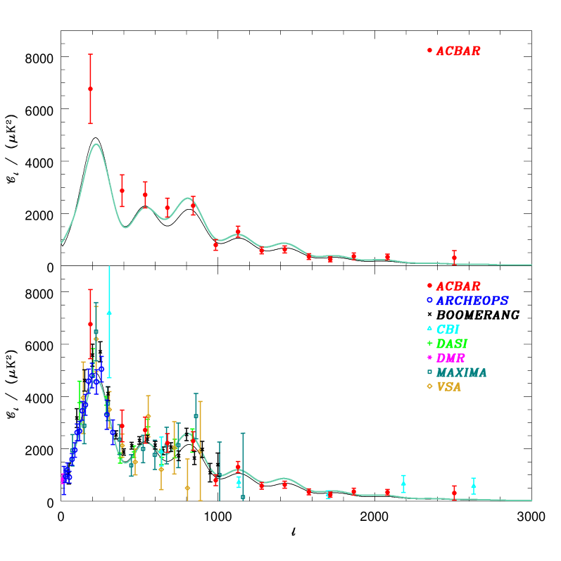
Figure 1: Top Panel: The Acbar CMB power spectrum, ${\mathcal{C}}_{\ell}\equiv\ell(\ell+1)C_{\ell}/{(2\pi)}$, plotted over a vacuum energy dominated [$\Omega_{k}=-0.05$, $\Omega_{\Lambda}=0.5$, $\omega_{cdm}=0.12$, $\omega_{b}=0.02$, $H_{0}=50$, $\tau_{C}=0.025$, $n_{s}=0.925$, amplitude ${\sqrt{\mathcal{C}}_{10}}=1.11\times 10^{-5}T_{\rm CMB}$] model (black thin line) and a CDM dominated [$\Omega_{k}=0.05$, $\Omega_{\Lambda}=0$, $\omega_{cdm}=0.22$, $\omega_{b}=0.02$, $H_{0}=50$, $\tau_{C}=0$, $n_{s}=0.925$, amplitude ${\sqrt{\mathcal{C}}_{10}}=1.34\times 10^{-5}T_{\rm CMB}$] model (green thick line). These are the best-fit models, for $\Lambda$ and $\Lambda$-free models respectively, found during the Acbar+Others parameter estimation described in the text, with the weak-$h$ prior. Bottom Panel: The top panel with the addition of power spectra from several other experiments. Both models appear to be reasonable fits to the data, with the $\Omega_{\Lambda}=0.5$ model statistically being the better of the two.

The results of Paper I provide 14 “band powers” with effective centers between $\ell=190$ and 2500. Figure 1 shows these results, along with a selection of other current measurements for context and comparison. The points plotted in Figure 1 lie at the maxima $\overline{{\mathcal{C}}}_{B}$ of the joint likelihood distribution ${\mathcal{L}}(\{{\mathcal{C}}_{B})$ for each band power (${\mathcal{C}}_{B}$), with the vertical bars showing errors derived from the curvature of the likelihood at that maximum,

$${\mathcal{F}}_{BB^{\prime}}^{({\mathcal{C}})}=-\frac{\partial^{2}\ln{{\mathcal{L}}({\mathcal{C}}_{B})}}{\partial{\mathcal{C}}_{B}\partial{\mathcal{C}}_{B^{\prime}}}\ .$$ (1)

The errors shown are Gaussian ones, $[{\mathcal{F}}^{-1/2}]_{BB}$. For Acbar, the curvature matrix determined from the original bands has been rotated into the diagonal frame, with eigenvalues $f_{B}$. Figure 1 shows $f_{B}^{-1/2}$ for the errors. For the other experiments shown, the results are not rotated to the diagonal frame.

Of course the likelihood curves for the individual bandpowers are not Gaussians. An offset lognormal distribution (Bond et al., 2000) has been shown to be an accurate representation of the likelihood curves, and is used in all of our parameter estimations. This distribution is Gaussian in the variables

$$Z_{B}=\ln{({\mathcal{C}}_{B}+x_{B})}\ .$$ (2)

Here, $x_{B}$ represents a noise contribution to the band power. For Acbar, $x_{B}$ was treated as a parameter determined by fitting the lognormal distribution to the likelihood, as described in in Paper I. $\overline{{\mathcal{C}}}_{B}$, $f_{B}^{-1/2}$, and $x_{B}$ are given in Table 2 of that paper.

4 Comparison with Theory

For the standard cosmological model with adiabatic initial density perturbations, the CMB angular power spectrum can be readily calculated as a function of input cosmological parameters $\vec{y}$. These theoretical predictions for $C_{\ell}$ can be made individually for each $\ell$, while our measurement is over bands of finite width, characterized by the window functions $\varphi_{B\ell}$. Given the theoretically predicted $C_{\ell}$, the predicted band power ${\mathcal{C}}_{B}$ in one of our bands is

$${\mathcal{C}}_{B}\equiv{\mathcal{I}}(\varphi_{B\ell}{\mathcal{C}}_{\ell})/{\mathcal{I}}(\varphi_{B\ell})\ ,$$ (3)

where ${\mathcal{C}}_{\ell}\equiv\ell(\ell+1)C_{\ell}/2\pi$ and

$${\mathcal{I}}(f_{\ell})\equiv\sum\limits_{\ell}\frac{(\ell+\frac{1}{2})}{\ell(\ell+1)}f_{\ell}\ .$$ (4)

The window functions $\varphi_{B\ell}$ give the response of the bands to power at each $\ell$. Numerical tabulations of the window functions are available on the Acbar experiment public website. They have been rotated into the diagonal frame.

The likelihood that the data would result from the cosmology described by $\vec{y}$ is given by

$$\begin{split}\ln{\mathcal{L}}({\bf{\mathcal{C}}})=&\ln{\mathcal{L}}(\overline{{\bf\mathcal{C}}})-\\ &\frac{1}{2}\sum\limits_{BB^{\prime}}(Z_{B}-\overline{Z}_{B}){\mathcal{F}}_{BB^{\prime}}^{(z)}(Z_{B^{\prime}}-\overline{Z}_{B^{\prime}})\ ,\end{split}$$ (5)

where $\overline{Z}_{B}=\ln{(\overline{{\mathcal{C}}}_{B}+x_{B})}$ is the value of the lognormal parameter at the position of maximum likelihood $\overline{{\mathcal{C}}}_{B}$ and ${\mathcal{F}}_{BB^{\prime}}^{(z)}$ is the curvature matrix transformed into the lognormal variables,

$${\mathcal{F}}_{BB^{\prime}}^{(z)}=(\overline{{\mathcal{C}}}_{B}+x_{B}){\mathcal{F}}_{BB^{\prime}}^{({\mathcal{C}})}(\overline{{\mathcal{C}}}_{B}^{\prime}+x_{B}^{\prime})\ .$$ (6)

Provided with the maximum likelihood band powers $\overline{{\mathcal{C}}}_{B}$, the lognormal offsets $x_{B}$, the curvature matrix ${\mathcal{F}}_{BB^{\prime}}^{({\mathcal{C}})}$, and the window functions $\varphi_{B\ell}$, the likelihood of the parameter set $\vec{y}$, given the data, can be computed.

Our set $\vec{y}$ consists of seven cosmological parameters: $\Omega_{k}=(1-\Omega_{tot}),\Omega_{\Lambda},\omega_{cdm},\omega_{b},n_{s},\tau_{C},\ln{{\mathcal{C}}_{10}}$. The total energy density of the universe in units of critical density $\Omega_{tot}$ is linked to the global curvature of space: negatively curved for $\Omega_{tot}<1$, positively curved for $\Omega_{tot}>1$ and flat for $\Omega_{tot}=1$. The total energy density has 3 constituents: vacuum ($\Omega_{\Lambda}$), matter and relativistic particles. The relativistic energy density is currently negligible. The matter density is split into two types, baryonic matter ($\Omega_{b}\equiv\omega_{b}/h^{2}$), which interacts with electromagnetic radiation, and cold dark matter ($\Omega_{cdm}\equiv\omega_{cdm}/h^{2}$), which does not. The total matter density is denoted $\Omega_{m}=\Omega_{b}+\Omega_{cdm}$. The amplitude of the CMB power spectrum at $\ell=10$, $\ln{{\mathcal{C}}_{10}}$ gives the overall amplitude of the primordial fluctuations. This quantity is well-constrained by the COBE-DMR observations (Bennett et al., 1996). The full COBE-DMR power spectrum as described in Bond et al. (2000) is included in all of our parameter analyses. The spectral index of primordial density perturbations, $n_{s}$, parameterizes the variation in the fluctuation power as a function of length scale; $n_{s}=1$ corresponds to scale invariance.

The universe reionized at some point between decoupling and the present. After reionization, CMB photons scatter further. $\tau_{C}$ is the Compton optical depth (from decoupling to present) due to such scattering. High $\tau_{C}$ diminishes CMB power by a factor of $\exp[-2\tau_{C}]$ over most of the $\ell$ range, though not in the DMR range.

Many more parameters than our basic 7 may be needed to completely describe inflationary models. These include the gravity-wave induced tensor amplitude and tilt, variations of tilt with wavenumber, relativistic particle densities, more complex dynamics associated with the dark energy $\Omega_{\Lambda}$, etc. For example, a gravity-wave induced component is expected in the largest class of inflation models, and has impact on the spectrum in the $\ell<100$ region. Although far from the region where Acbar has its impact, it can affect the amplitude, tilt, and Compton depth. If one constrains the tilts and amplitudes of the tensor component to those motivated by simple inflation models, there is little change in the other parameters.

It is possible that secondary anisotropies, such as the Sunyaev-Zeldovich effect investigated later in this paper, could contribute significant power to the highest $\ell$ band of our measurement. However, the detection of anisotropy in that band is only $1.1\sigma$, or $0.9\sigma$ above the best-fit model primary CMB angular power spectrum. Thus, for the purpose of cosmological parameter estimation from the primary CMB signal, we can safely ignore the effects of potential SZE contamination.

To derive estimates of cosmological parameters, we compare our data with the primary CMB power spectra predicted by combinations of cosmological parameters $\vec{y}$. In this comparison, we vary $\ln{{\mathcal{C}}_{10}}$ continuously, while the other parameters take the discrete values listed in Table 1. An angular power spectrum is generated for each set of discrete parameter values, forming a grid. Given a CMB dataset (e.g., Acbar or a combination of various measured power spectra), the likelihood is then calculated for each point on the seven dimensional grid.

To compute the likelihood that a particular parameter $X$ has a value $x_{0}$, the seven dimensional grid of likelihoods is integrated over the other six parameters, holding the parameter of interest fixed at $x_{0}$. This method, known as marginalization, involves calculating

$$L(X=x_{0})=\int\delta(X-x_{0})P_{prior}(\vec{y}){\mathcal{L}}(\vec{y})d\vec{y}\ ,$$ (7)

where $\delta(x)$ is the usual delta function and the prior $P_{prior}(\vec{y})$ is discussed below.

For each model on the parameter grid, along with the overall amplitude parameter ${\cal C}_{10}$, we continuously vary the beam widths $\sigma_{bi}$ and calibrations $A_{i}$ for each experiment $i$ about their estimated values $\overline{\sigma_{bi}}$ and unity, to take into account the uncertainties in the respective measurements. We approximate the beam-uncertainty and calibration-uncertainty “prior” probabilities by Gaussians in $\Delta(\sigma_{bi})^{2}$ and $\ln A_{i}^{2}$, respectively. The modification to the bandpower as a result of the uncertainty $\Delta(\sigma_{bi})^{2}$ is modeled by $\exp[-\langle(\ell+\frac{1}{2})^{2}\rangle_{B}\Delta(\sigma_{bi})^{2}]$, with $\langle(\ell+\frac{1}{2})^{2}\rangle_{B}={\mathcal{I}}(\varphi_{B\ell}(\ell+\frac{1}{2})^{2})/{\mathcal{I}}(\varphi_{B\ell})$. The overall impact of the calibration and beam uncertainties is that the combination $\ln{\cal C}_{10}+\sum_{i}\ln A_{i}^{2}-\langle(\ell+\frac{1}{2})^{2}\rangle_{B}\Delta(\sigma_{bi})^{2}$ is adjusted for each grid parameter combination to give the best fit with errors. Marginalization over the continuous parameters is done by calculating a Fisher matrix, and assuming a Gaussian distribution in the posterior distributions in the $\{\ln{\cal C}_{10},\ln A_{i}^{2},\Delta(\sigma_{bi})^{2}\}$ variables. Marginalization over the grid parameters is done by discrete integration.

In addition to the parameters given in Table 1, we examine four “derived” parameters, which are functions of our basic 7 variables, $\{t_{0}$, $h$, $\sigma_{8}^{2}$, and $\Gamma_{\rm eff}\}$. Here $h$ is the value of the Hubble expansion parameter, $H_{0}=100~{}h$ km/s/Mpc and is given by

$$h={\sqrt{\frac{\omega_{b}+\omega_{cdm}}{1-\Omega_{k}-\Omega_{\Lambda}}}}\ .$$ (8)

The age of the universe is

$$t_{0}({\rm Gyr})\approx\frac{9.778}{h}\int_{0}^{1}\frac{2x^{2}}{\sqrt{\Omega_{m}+\Omega_{k}x^{2}+\Omega_{\Lambda}x^{3}}}dx\ ,$$ (9)

where we have dropped the minor effects of relativistic particles here, but not when we do our actual comparisons. The variance in the (linear) density fluctuation spectrum on the scale of clusters of galaxies ($8h^{-1}$ Mpc) is $\sigma_{8}^{2}$. The shape of the linear density power spectrum is described by the parameter

$$\begin{split}&\Gamma_{\rm eff}=\Gamma+(n_{s}-1)/2,\quad{\rm where}\\ &\Gamma=\Omega_{m}\,h\,\,e^{-(\Omega_{b}(1+\Omega_{m}^{-1}\sqrt{2h})-0.06)}\ .\end{split}$$ (10)

Note that $\Gamma_{\rm eff}\approx\Omega_{m}h$ with corrections due to baryon density and spectral tilt $n_{s}$ over the region probed by large scale structure observations that approximate the dominant dependences. The derived parameters are not marginalized over, and do not define dimensions in the parameter grid because they are determined given a set of parameters $\vec{y}$. The derived parameters are calculated at each point on the model grid. We can make Bayesian estimates of those parameters using equation (7) with $X$ being the derived parameter of interest.

We can also use the derived parameters to account for other cosmological information. Estimates of these parameters from other, non-CMB, observations can be included as “prior constraints”. Equation (7) is cast in a form that gives a likelihood as a function of our parameters, and priors $P_{prior}(\vec{y})$.

All our analyses include the loose prior implicitly imposed by the edges of the database given in Table 1, and two other very weak priors that are generally accepted by most cosmologists: models are restricted to those where the current age of the universe is $t_{0}>10$Gyr, and where the matter density $\Omega_{m}$ is greater than 0.1.

We add to these constraints a series of additional priors:

• weak-h : $0.45<h<0.90$. This is a tophat restriction, designed to allow the CMB data, rather than arguable priors, to drive the results.

• LSS : We employ two constraints based on large scale structure (LSS) observations, on the combinations $\sigma_{8}\Omega_{m}^{0.56}$ and $\Gamma_{\rm eff}$. For both priors, we adopt a Gaussian distribution convolved with a top-hat distribution, characterized by the parameters $\sigma_{8}\Omega_{m}^{0.56}=0.47_{-.02,-.08}^{+.02,+.11}$ and $\Gamma_{\rm eff}=0.21_{-.03,-.08}^{+.03,+.08}$, where the first error gives the 1-$\sigma$ point of the Gaussian distribution, and the second error gives the extent of the tophat distribution. Our basic philosophy is to adopt priors that are not overly restrictive since the LSS data is still improving. The motivation for the choice and the discussion of the LSS data is given in Bond et al. (2002a). The $\Gamma_{\rm eff}$ distribution encompasses recent results from the 2dF and SDSS surveys. The $\sigma_{8}$ distribution encompasses results from recent weak lensing surveys. It also covers many of the cluster abundance determinations using X-ray temperature and other cluster data.

• LSS($low$–$\sigma_{8}$): There are currently a few cluster abundance estimations that point to values of $\sigma_{8}$ that are lower than the weak lensing estimates. Although our standard LSS prior takes most of these variations into account by its spread, we have also tested the effect of shifting the entire $\sigma_{8}$-distribution downward by 15%, to $\sigma_{8}\Omega_{m}^{0.56}=0.40_{-.02,-.08}^{+.02,+.11}$. We keep the $\Gamma$ prior the same.

• HST-h : We strengthen our $h$ prior, based on the Hubble Space Telescope Key Project measurement (Freedman et al., 2001) of the Hubble constant, $h=0.72\pm 0.08$. This is a Gaussian prior with the stated error as the 1–$\sigma$ points.

• Strong data : We combine the LSS prior given above with the HST-$h$ prior, and add a constraint (in the $\Omega_{\Lambda}$ vs. $\Omega_{tot}$ plane) based on surveys of the brightness vs. redshift relation of Type 1a Supernovae (Perlmutter & Riess, 1999; Riess et al., 1998).

• Flat : Inflation models generally predict a flat geometry, and recent evidence supports this (eg de Bernardis et al., 2000; Halverson et al., 2001). For the converted, we investigate the effects of holding $\Omega_{tot}$ equal to one.

5 Constraints on Cosmological Parameters from CMB Spectra

We apply these methods to three combinations of CMB data, using a series of priors for each case. By doing so, we can investigate the power of adding Acbar data to the current cosmological mix, as well as the dependence of results on the strength and nature of the applied priors.

The full COBE-DMR power spectrum of Bond et al. (1998) is included in all our analyses. The first combination of CMB data, Acbar+DMR, investigates the potential for using the DMR low-$\ell$ anchor with the damping-tail measurement of Acbar as an independent check on previous CMB-based cosmological parameter estimation.

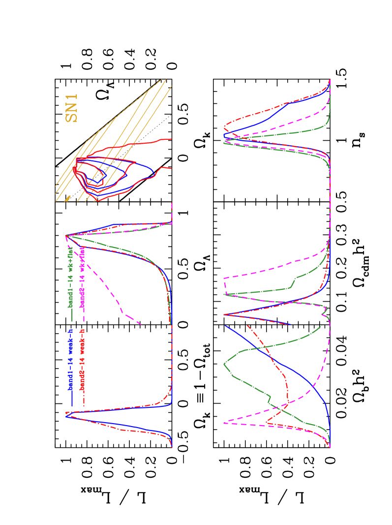
Figure 2: Likelihood curves for Acbar+DMR with the $weak$ and $weak$+flat priors. Each prior case is plotted with and without the first Acbar band (centered on $\ell=187$) included in the analysis. In the upper–right panel, the 1 to 3-$\sigma$ contours are shown for the 2D $\Omega_{k}$–$\Omega_{\Lambda}$ likelihood with the $weak$ prior and bands 1-14 (blue) and bands 2-14 (red). The thick black lines define $\Omega_{m}=0$ and $\Omega_{m}=1$ and the dotted black line defines $\Omega_{m}=0.5$. The yellow contours are the 1, 2 and 3-$\sigma$ levels of constraints based on Type 1a Supernovae. The lack of stability of the curves (for $\omega_{b}$ in particular) indicates that Acbar+DMR alone is not sufficient for robust parameter estimation.

Figure 2 shows marginalized likelihood curves for Acbar and DMR only, using the weak-$h$ and weak-$h$+flat priors. These are displayed for each of two sets of Acbar data, the first being the full spectrum (bands 1-14), the second being bands 2-14. The curves show the parameter estimates are very prior-dependent, and also depend upon whether we include the lowest $\ell$ band data, despite the large errors in that band. These variations are a result of Acbar not pinning down the peak/dip structure well. Parameter estimates are then relying more on the specific shape of the damping tail.

The physics of damping is well known and clearly depends upon the cosmological parameter characterizing the strength of the viscous and diffusive couplings, $\omega_{b}$. It might then be thought that by using only Acbar and DMR we could get a strong constraint on this parameter. However, when we take account of all of the influences that determine the damping scale in $\ell$-space, it is found to be relatively insensitive (see e.g., Sievers et al. (2002) for a discussion). Once some information is given on the peak/dip structure that helps to pin the parameters, Acbar improves the quality of the determinations by virtue of its small error bars in the damping tail region. We therefore proceed by including CMB data in the $\ell$ range between DMR and Acbar, over the first three acoustic peaks.

Many CMB experiments have made sensitive measurements of the power spectrum in the region of those peaks; we choose here to combine the low-$\ell$ measurement of DMR with a set of recent higher-$\ell$ observations, comprised of Archeops (Benoit et al., 2002), Boomerang (Ruhl et al., 2002), DASI (Halverson et al., 2001), MAXIMA (Hanany et al., 2000), and VSA (Scott et al., 2002). We also include the recent high-$\ell$ results of CBI (Pearson et al., 2002). We give the label “Others” to this aggregate set of data and first investigate the parameter extraction that can be done with these measurements, sans Acbar. Finally, we investigate the improvements made when adding Acbar to the mix, in a combination we label “Acbar+Others”.

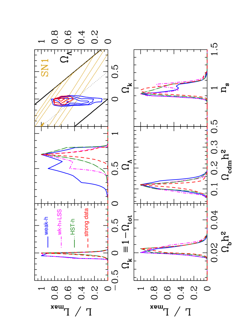
Figure 4: Likelihood curves for Acbar +Archeops+B98+CBI+DASI+DMR+MAXIMA+VSA (Acbar+“Others”) with the $weak$, $weak$+LSS, HST–$h$, and strong data priors. The $\Omega_{k}$–$\Omega_{\Lambda}$ contours are shown for the $weak$ (blue) and strong data (red) cases. The yellow contours are the 1, 2 and 3-$\sigma$ levels of constraints based on Type 1a Supernovae. The positions and widths of these curves do not differ significantly from those in Figure 3 despite the addition of the low noise Acbar data through the damping tail. A comparison of the curves here containing the LSS prior ($weak$+LSS and strong data) with those derived using the a lower estimate (discussed in the text) shows only small changes. The most noticeable changes are an upward shift in the lower tail on $\Omega_{\Lambda}$, and a broader and higher–value $n_{s}$ peak. Table 2 gives numerical estimates of these parameters, derived by integration of these curves.

Two plots of one-dimensional marginalized likelihood curves, for “Others” and “Acbar+Others”, are given in Figures 3 and 4 respectively. Here we see that results are generally stable to the application of priors - that is, the application of a prior may narrow the result, but does not move it outside the range imposed by other priors.

It is remarkable how many parameters are well constrained in Figures 3 and 4. Using only a weak-$h$ prior, four of the five parameters shown ($\Omega_{k}$, $\Omega_{b}h^{2}$, $\Omega_{cdm}h^{2}$, and $n_{s}$) are well localized. The detection of $\Omega_{\Lambda}$ becomes stronger as stronger priors are applied.

We have investigated the effects of dropping the first Acbar bin on the results shown in Figure 4, and unlike the Acbar+DMR results, the effects of this action are negligible. This is not surprising, given that the first peak information in “Others” and “Others+Acbar” is driven by the other measurements.

The likelihood curves shown in these figures can be used to find confidence intervals on each parameter for each prior. We can proceed in a similar way to constrain the values of other parameters, such as $h$ and the current age of the universe ($t_{0}$). Table 2 gives the median values and 1-$\sigma$ limits (16% and 84% integrals of the likelihood) for a set of cosmological parameters. For $\tau_{C}$, the 95% confidence upper limit is given. A comparison of the values in the Table, or of Figures 3 and 4, shows that the impact of adding Acbar to this mix is not dramatic. There are modest improvements in some parameter estimates, most notably $\Omega_{\Lambda}$ and $\Omega_{cdm}h^{2}$.

Not immediately obvious from the figures is the improved rejection of $\Omega_{\Lambda}=0$ models. One measure of this is the improvement in the 3-$\sigma$ lower limit on $\Omega_{\Lambda}$, found by integrating the likelihood curve. This 3-$\sigma$ limit improves from $\Omega_{\Lambda}>0.086$ for “Others” to $\Omega_{\Lambda}>0.136$ for “Acbar+Others”; that is, the probability of having a lower value of $\Omega_{\Lambda}$ than these is $0.14\%$. This depends upon the specific range in $h$ we are allowing in our weak prior.

The source of this rejection of models near $\Omega_{\Lambda}=0$ can be illustrated by examining the $\chi^{2}$ of the aggregate dataset to the best-fit models, in both the $\Omega_{\Lambda}=0$ and the “free” $\Omega_{\Lambda}$ cases. We find, for the “Acbar+Others” dataset (consisting of 116 band powers) $\chi^{2}=140$ and $\chi^{2}=160$ for the best-fit “free $\Omega_{\Lambda}$” and $\Omega_{\Lambda}=0$ models, respectively. Thus, while both models plotted in Figure 1 appear reasonable to the eye, the fit is significantly better for the $\Omega_{\Lambda}=0.5$ model.

Unfortunately, calculating the effective number of degrees of freedom in this $\chi^{2}$ is not straightforward. Taking beam and calibration uncertainties for each observation as a total of 16 parameters in the fit added to the 7 cosmological parameters, we know the effective degrees of freedom lies in the range $93<\mbox{dof}<116$. Adopting dof=100 as a reasonable estimate, the probability of finding $\chi^{2}>140$ and $\chi^{2}>160$ are $P_{>}=0.0051$ and 0.00013 respectively. We caution the reader against strict interpretation of these statistically high $\chi^{2}$ in the face of this very heterogeneous data set. Instead, we note the significant improvement in $\chi^{2}$ enabled by the addition of a single parameter in the fit.

Interestingly, the $\chi^{2}$ difference of the best-fit models is roughly consistent with the ratio of the marginalized likelihoods (for the weak-$h$ prior) at the peak of the likelihood curve near $\Omega_{\Lambda}=0.7$ and its level at $\Omega_{\Lambda}=0$. Exact correspondence would be expected if our parameter likelihood function had a Gaussian form.

One would think that the information Acbar adds at high $\ell$ would significantly improve the determinations of $\omega_{b}$ because of viscous damping and $n_{s}$ just because of the increased $\ell$-baseline. This is clearly not the case. We have discussed the damping tail issue already. The near degeneracies due to correlations among certain parameter combinations imply that increased data does not necessarily lead to increased precision on the cosmological parameters. It is likely that the lack of improvement in these projections to individual parameters is due to degeneracies in the parameter space.

Such degeneracies are well known and have been discussed at length in the literature; see Efstathiou & Bond (1999) for an extensive treatment of some of the most pernicious of these. For example, one of these (the “geometric degeneracy”), leads to nearly identical angular power spectra for particular combinations of ($\Omega_{\Lambda}$, $\Omega_{k}$, $\Omega_{m}$, $h$), while leaving $\omega_{b}$ and $\omega_{cdm}$ fixed. The breaking of this geometric degeneracy is the reason estimates of $\Omega_{\Lambda}$ and, to a lesser extent $\Omega_{cdm}h^{2}$, improve so dramatically as stronger priors on $h$ are applied. Other less exact degeneracies, such as one between amplitude, $n_{s}$ and $\tau_{C}$, lead to similar broadenings of these projected likelihood curves.

By choosing our database parameters well (e.g., using the physical densities $\omega_{b}$ and $\omega_{cdm}$ rather than the densities relative to critical) we have minimized the effects of some potential degeneracies. By exploring the parameter eigenmodes we can escape the limitations of the canonical parameters and determine the true power of any combination of datasets. This process is in fact quite familiar to most cosmologists; the Type 1a supernovae results are often considered as limiting the parameter “eigenmode” $\Omega_{\Lambda}$–$\Omega_{M}$.

Table 3 lists the best-determined five (of seven total) eigenmodes for the “Others” and “Acbar+Others” analyses. The coefficients describing those modes, and the errors on the eigenvalues, are determined by ensemble averages of the likelihood derivatives over the parameter database. We introduce the probability-weighted ensemble average of a parameter $y_{a}$,

$$\left<y_{a}\right>=\int y_{a}P_{prior}(\vec{y}){\cal L}(\vec{y})d\vec{y}\ ,$$ (11)

and the probability weighted ensemble average of the differentials

$$\left<\delta y_{a}\,\delta y_{b}\right>=\int\delta y_{a}\delta y_{b}P_{prior}(\vec{y}){\cal L}(\vec{y})d\vec{y}\ ,$$ (12)

where $\delta y_{a}\equiv y_{a}-\left<y_{a}\right>$.

The eigenmodes themselves ($\xi_{k}$) and their errors ($\sigma^{\xi}_{k}$) are given by the application of a rotation matrix ${\bf R}$ to the parameter vector $\vec{y}$,

$$\xi_{k} = \sum_{a}R_{ak}\delta y_{a}\ ,$$ (13)

$$\left<\delta y_{a}\delta y_{b}\right> = \sum_{k}R_{ak}(\sigma^{\xi}_{k})^{2}R_{bk}\ .$$ (14)

In this eigenmode analysis, we have used the fractional deviations $\delta\omega_{b}/\left<\omega_{b}\right>$ and $\delta\omega_{cdm}/\left<\omega_{cdm}\right>$ as parameters, rather than $\omega_{b}$ and $\omega_{cdm}$, to set their deviation magnitudes on more equal footing with those of the other parameters.

Inspection of the table shows that while the eigenmodes for “Others” and “Acbar+Others” are not identical, they are very similar. In most cases they are dominated by contributions from one or two cosmological parameters, but in all cases there are significant components from several parameters. The table shows much more clearly the impact of adding Acbar to the dataset; all of the eigenvalue uncertainties improve, but the greatest improvement is in the fifth eigenmode, which becomes the fourth one when Acbar is added. It is dominated by the cosmological constant.

6 Constraints on $\sigma_{8}$ from the Sunyaev-Zeldovich Effect

The Acbar results provide the first data above $\ell=2000$ at 150 GHz. The recent CBI Deep field results (Mason et al., 2002), at 30 GHz, have indicated a possible excess over the expected primary anisotropy signal at $\ell>2000$. The most promising candidate for the source of the excess is the Sunyaev-Zeldovich Effect (SZE) due to the scattering of CMB off hot electrons in the intra-cluster medium (see Birkinshaw (1999) for a recent review). The CBI results have been interpreted in the context of the SZE with tentative constraints being obtained on the value of $\sigma_{8}$ (Bond et al., 2002a; Komatsu & Seljak, 2002; Holder, 2002). The BIMA array (Dawson et al., 2002), operating at 30 GHz, has also reported detection of power at higher $\ell$ which also has been attributed to the SZE by Komatsu & Seljak (2002).

Parameter fitting using secondary effects such as the SZE must be approached with caution. Both numerical and analytical predictions for the SZE power spectrum suffer from a number of uncertainties. The results of different simulations, although in general agreement, show significant differences in both the amplitude and shape of the predicted spectrum. Analytical models suffer from uncertainties inherent in modeling the profile of the clusters. In addition, cooling and heating effects in the clusters are not yet well understood and most simulations and analytical models do not take these effects into account. Simulations have shown that for modest deviations about the concordance $\Lambda CDM$ model, the SZE angular power spectrum scales as ${\cal C}^{\rm SZ}_{\ell}\sim(\Omega_{b}h)^{2}\sigma_{8}^{7}$. Despite uncertainties in the physics of cluster models, especially the role of energy injection, and the relatively large errors on the observations, this very strong dependence of the SZE spectrum on $\sigma_{8}$ enables the derivation of significant constraints on $\sigma_{8}$ from current data.

We choose to model the SZE using two angular power spectrum templates. The first is obtained from large Smoothed Particle Hydrodynamics (SPH) simulations of $\Lambda CDM$ (Bond et al., 2002b; Wadsley et al., 2002). The second is obtained from an analytical model (see Zhang et al. (2002); Bond et al. (2002a) for details). Both templates were scaled to a fiducial value of $\Omega_{b}h=0.035$.

Although the power in the primary spectrum is falling rapidly compared to the rising contribution of the SZE at $\ell>2000$, interpretation of the low noise Acbar band powers around the cross-over region is sensitive to the contribution of the primary signal together with the secondary. Rather than consider a full range of parameter space we select a simple model for the primary spectrum, a best fit flat model for the “Acbar+Others” data combination ($\Omega_{b}=0.047$, $\Omega_{cdm}=0.253$, $\Omega_{\Lambda}=0.7$, $h=0.69$, $n_{s}=0.975$ and $\tau_{C}=0.2$). The primary model was normalized with the best fit amplitude obtained from the fits. However, uncertainties in the model parameters affect the overall amplitude of the primary spectrum at scales $\ell\approx 2000$ where the primary and secondary signals are comparable. We chose to parameterize the freedom in the primary and secondary spectra by two effective parameters, an amplitude in the primary power spectrum $q_{2K}^{\rm eff}$ and a scaling factor for the SZE $\sigma_{8}^{\rm SZ}$. Uncertainty in the primary parameter $q_{2K}^{\rm eff}$ represents the uncertainties in a number of dominant effects given by the combination of parameters: $\sigma_{8}$, $\tau_{C}$, and $n_{s}$, as shown in section 5. Most significantly, it also incorporates the effect of systematic uncertainties such as an overall calibration and beam uncertainty in the data. The secondary amplitude parameter $\sigma_{8}^{\rm SZ}$ describes the scaling of the SZE spectrum and can be related to $\sigma_{8}$ via $\sigma_{8}^{\rm SZ}\approx(\Omega_{b}h/0.035)^{0.29}\sigma_{8}$.

We select points with $\ell>1500$ for fitting and use the offset lognormal approximation as described in Section 3. The target model is now $Z^{T}_{B}=\ln({\cal C}_{B}+g_{\nu}{\cal C}_{B}^{\rm SZ}+x_{B})$ where the primary and SZE spectra have been filtered by the appropriate window functions for each band power and $g_{\nu}$ is the frequency dependent scaling of the SZE (a factor of $\sim 4$ in power lower at 150GHz compared to 30GHz). Top–hat windows are used to model the BIMA band powers. The primary model is scaled by $q_{2K}^{\rm eff}$ over the range $(0.1,1.8)$ and the secondary model is scaled by $\sigma_{8}^{\rm SZ}$ over the range $(0.5,1.4)$. At each point in the grid, we calculate the quantity $-2\ln(L)$ for the model.

To assign a realistic uncertainty to the amplitude of the primary models, we add a Gaussian prior in the amplitude $q_{2K}^{\rm eff}$ with a width of 20% RMS. This is chosen to reflect the uncertainty in the amplitude of the best fit models obtained in the parameter fits described in section 5. As an example, the Acbar data fixes the amplitude of our template model with an RMS of 17% while the CBI Deep field data fixes the same model with an RMS of 21%. We check that our results are robust to a change in the width of the prior by fitting with a 10% and 40% RMS width. The marginalized, best fit value, and upper errors for $\sigma_{8}^{\rm SZ}$ reported below changes by only 0.1% while the lower error changes by 1% on average.

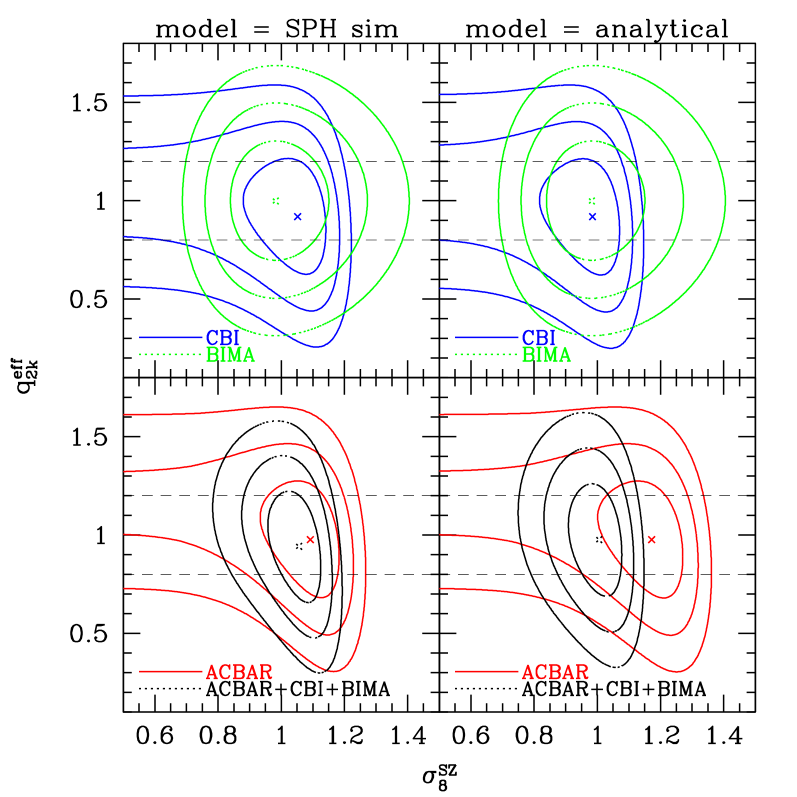
Figure 5: 1, 2, and 3–$\sigma$ contours for various combinations of data sets in the $(q_{2K}^{\rm eff},\sigma_{8}^{\rm SZ})$ plane. The left panels show fits obtained using the SPH template and the right panels are the equivalent for the analytical model. Both CBI and Acbar data points constrain the upper values of $\sigma_{8}^{\rm SZ}$ but not the lower values as they are sensitive to the amplitude of the primary spectrum. The higher–$\ell$ BIMA observations are insensitive to the primary component and therefore provide a strong lower bound. The combination of the three datasets (bottom row – dotted, black contours) show a strong detection of the SZ component. The dashed parallel lines show the width of the Gaussian prior imposed on $q_{2K}^{\rm eff}$. We use a lognormal distribution for the BIMA band powers.

In Fig. 5 we show contour plots of the $\chi^{2}$ grids in the ($q_{2K}^{\rm eff}$, $\sigma_{8}^{\rm SZ}$) plane. We subtract the $\chi^{2}$ value at the minimum from the grids and the (2.3, 6.17, 11.8) contours give an indication of where the 1, 2, 3–$\sigma$ levels would fall if the likelihoods were Gaussian. We show results for both template models used in the analysis. The contours show that the data is only weakly dependent on the $q_{2K}^{\rm eff}$ amplitude with a slight movement to higher $\sigma_{8}^{\rm SZ}$ for low $q_{2K}^{\rm eff}$ as expected for Acbar and CBI data. This reflects the fact that the only bands sensitive to the primary amplitude are the lowest $\ell$ bands included from the Acbar and CBI data. The high–$\ell$ BIMA data is fully degenerate in the amplitude of the primary, as expected, and the contours in the $q_{2K}^{\rm eff}$ direction simply reflect the Gaussian prior. It does however give a strong lower bound although this depends strongly on the lognormality of the BIMA band power distribution. The $x_{B}$ offsets are not available for BIMA and are set to $x_{B}=0$ although we also show results where no lognormal transformation was applied to the BIMA points (Table 4). Acbar and CBI provide strong upper bounds. A combination of the three data sets give strong constraints in $\sigma_{8}^{\rm SZ}$ with the contours showing a slight tilt in the expected direction with respect to $q_{2K}^{\rm eff}$.

One major obstacle in using a secondary effect such as the SZE to fit parameters is the non-Gaussian nature of the signal from non-linear structures such as clusters. In general the non-Gaussianity will increase the sample variance of the underlying signal. Treating the data as Gaussian can therefore result in an overestimate of the significance of the constraint. This effect has been investigated using numerical simulations of the SZE (White et al., 2002; Zhang et al., 2002) and also by calculating the contribution to the covariance by the fourth order, trispectrum term $T_{\ell\ell^{\prime}}$ (Cooray, 2001; Komatsu & Seljak, 2002). In general the sample variance is found to be a factor $\sim 3$ higher than the Gaussian equivalent with some dependence on $\ell$ and also on the width of the bands being considered ($\ell$-$\ell^{\prime}$ correlations are also altered by the non-Gaussianity). In order to include this effect in the errors and correlations we scale the inverse Fisher matrix of the band powers as

$${\cal\bar{F}}_{BB^{\prime}}^{-1}\equiv f^{\rm ng}_{B}{\cal F}_{BB^{\prime}}^{-1}f^{\rm ng}_{B^{\prime}}\ ,$$ (15)

where $f^{\rm ng}_{B}$ is the scaling factor. Here we chose $f^{\rm ng}_{B}$ such that the sample variance component of the error is a factor of 3 larger than the expected Gaussian case which can be approximately evaluated as

$$\Delta C_{\ell}\approx\frac{\sqrt{2}C_{\ell}}{\sqrt{f_{\rm sky}\Delta_{B}(2\ell_{b}+1)}}\ .$$ (16)

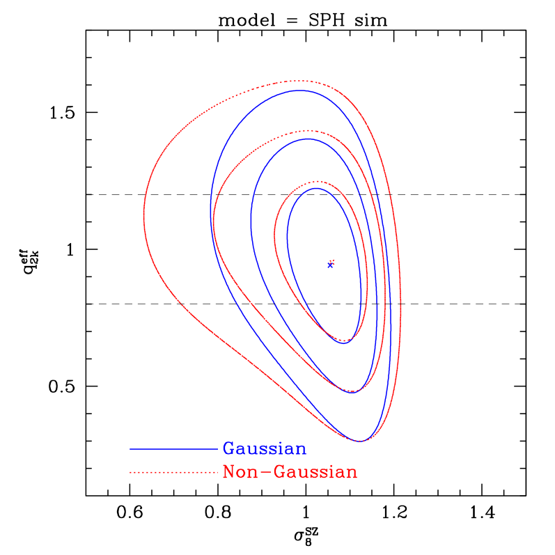
Figure 6: The plot shows the effect of adding a correction for the increased sample variance of the data due to the non–Gaussian scatter. Both contours are for the combination Acbar+CBI+BIMA. The effect is significant, particularly at the 3–$\sigma$ level.

Fig. 6 shows the effect of the correction on ($q_{2K}^{\rm eff}$,$\sigma_{8}^{\rm SZ}$). In general the correction changes from experiment to experiment and from band to band due to the different sample variance component in the uncertainty of each band. It is therefore important to include this effect in the analysis since it can have a substantial effect on the structure of the contours as opposed to a simple rescaling of the confidence limits. We find that the correction has significant effects on the allowed region, particularly at the 2 to 3-$\sigma$ level.

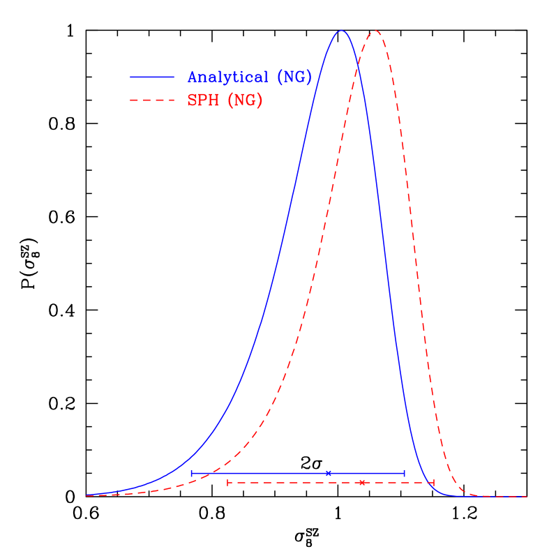
Figure 7: Marginalized likelihoods for the Acbar+CBI+BIMA combination. The results of fits using both the SPH (red, dashed) and analytical (blue, solid) models are shown. Both cases include non–Gaussian corrections. The 2–$\sigma$ upper and lower bounds and median values were obtained by computing the 2.5%, 97.5%, and 50% integrals of the likelihoods respectively. We find that the SPH model prefers slightly higher values for $\sigma_{8}^{\rm SZ}$. This is due to the fact that the SPH spectra show less power than the analytical models on large scales.

To obtain best estimates on the value of $\sigma_{8}^{\rm SZ}$, we marginalize over the $q_{2K}^{\rm eff}$ direction to recover the one dimensional likelihood in $\sigma_{8}^{\rm SZ}$. We show the resulting likelihoods in Fig. 7 for both analytical and SPH templates. Both results include the non-Gaussian correction discussed above. The 2-$\sigma$ region and median values shown as errorbars are obtained by calculating the $2.5\%$, $97.5\%$ and $50\%$ integrals of the likelihoods respectively. The results for both templates with 2-$\sigma$ error estimates are summarized in Table 4. We find that fitting with the SPH template results in values for $\sigma_{8}^{\rm SZ}$ about 6% higher than when the analytical model is used. This effect is due to the SPH model having a lower amplitude at larger scales than the analytical model (Fig. 8).

In Fig. 8 we show the primary and SZE templates used, scaled to the best fit value of $\sigma_{8}^{\rm SZ}=0.98$ (at 30GHz and 150GHz) for the analytical case shown in Fig. 7. The total primary+SZE (analytical) model is also shown together with the SPH template scaled to the same parameters. We see that the method can obtain a good fit between the data and primary+SZE model at both observing frequencies. Fig. 8 also shows the non-Gaussian corrections to each band power error.

It is important to note that if there is a non-negligible SZE component to the observed power, it may affect the parameter fits which assume only a primary contribution. However, the relative contribution to the Acbar band powers is very small, only approximately 15% in the last three bands. We do not expect this to have any significant impact on the parameter estimates derived in this work. As future observations increase the accuracy in this region of the spectrum, a fully consistent approach to parameter fitting will have to be adopted. Such an approach would simultaneously account for primary and secondary anisotropy, fitting for all parameters.

7 Conclusions

The Acbar data, the most sensitive to date in the damping-tail region, are in good agreement with predictions of flat $\Lambda$-CDM models with adiabatic initial perturbations. Considering the Acbar data together with other recent CMB results, we find that the addition of a single parameter to the model, $\Omega_{\Lambda}$, dramatically improves the best fit, with an improvement of $\Delta\chi^{2}=20$ upon adding that one parameter. Using very weak cosmological priors ($\Omega_{m}>0.1$, age $>10$Gyr, $0.45<h<0.90$), the 3-$\sigma$ lower limit on the cosmological constant rises to $\Omega_{\Lambda}>0.136$ upon including the Acbar data.

We find that the addition of Acbar data to the current CMB set does not lead to substantial improvements in the 1-$\sigma$ estimates of the canonical cosmological parameters. However, in an eigenmode analysis, the addition of Acbar data does improve the rotated parameter uncertainties, indicating that in this case the lack of improved errors on the pure cosmological parameters is probably dominated by degeneracies between those parameters.

We fit a SZE component to the data using Acbar and other measurements at high-$\ell$. Our estimates for the value of the effective quantity $\sigma_{8}^{\rm SZ}=(\Omega_{b}h/0.035)^{0.29}\sigma_{8}$ show an improvement over previous estimates using only CBI and BIMA observations. Although CBI and Acbar alone do not provide lower bounds on $\sigma_{8}^{\rm SZ}$, the combination of the two observations results in a detection greater than 3-$\sigma$ which is independent of the BIMA lower bound.

Our fits show that at a fiducial value of $\Omega_{b}h=0.035$ the central values for $\sigma_{8}$ are consistently higher than other estimates obtained using cluster data, weak lensing surveys and primary CMB observations (see Bond et al. (2002a) for a recent survey of $\sigma_{8}$ estimates). However, the results overlap with most other estimates at the 2-$\sigma$ level. As an indication, our LSS prior, a smoothed tophat on the combination $\sigma_{8}\Omega_{m}^{0.56}$, translates roughly into a smoothed tophat of $\sigma_{8}=0.92^{+0.21}_{-0.15}$ at $\Omega_{m}=0.3$. Any statistical inconsistency therefore, appears to be mild. Furthermore, systematic uncertainties in the estimates have not yet been taken into account. The difference displayed by the numerical and analytical based results of about 10% is indicative of the agreement between the two methods for predicting the SZE power spectrum (Komatsu & Seljak, 2002). In addition, entropy injection may have a significant effect on the SZE power spectrum. These effects would change the shape of the SZE template and impact directly on our determination of $\sigma_{8}$. Nevertheless, we conclude that the in the context of the phenomenological models adopted in this work, the data is consistent with a SZE component at $\sigma_{8}$ values near the high end of independent estimates.

Figure 3: Likelihood curves for Archeops+B98+CBI+DASI+DMR+MAXIMA+VSA (“Others”) with the $weak$, $weak$+LSS, HST-$h$, and strong data priors. The $\Omega_{k}$–$\Omega_{\Lambda}$ contours are shown for the $weak$ (blue) and strong data (red) cases. The yellow contours are the 1, 2 and 3-$\sigma$ levels of constraints based on Type 1a Supernovae. CMB estimates of $\Omega_{k}$, $\omega_{cdm}$, and $\omega_{b}$ are stable with sensible behavior as additional priors are employed.

Figure 8: Best fit primary+SZ model amplitudes. The top panel shows the SZ model scaled to an observing frequency of 30GHz which corresponds to the BIMA and CBI observations (first four rightmost points and two leftmost points respectively). The lower panel is for 150GHz, corresponding to the Acbar results. The solid lines show the analytical model at each frequency and the total primary+SZ. The dotted line shows the fiducial spectrum used to model the primary contribution at $\ell>1000$. The dashed line shows the SPH spectrum used as a template shape. The SZ contributions are scaled to a value of $\sigma_{8}^{\rm SZ}=0.98$ to show the amplitude at the best fit value obtained from the Acbar+CBI+BIMA combination using the analytic model as template (with non-Gaussian corrections). The extended errorbars for each point show the corrections due to the increase in sample variance expected from the non-Gaussian signal.

Table 1: Parameter Values Used in Grid

Parameter	Values
$\Omega_{k}$	$-0.5$	$-0.3$	$-0.2$	$-0.15$	$-0.1$	$-0.05$	$0$	$0.05$	$0.1$	$0.15$	$0.2$	$0.3$
	$0.5$	$0.7$	$0.9$
$\Omega_{\Lambda}$	$0$	$0.1$	$0.2$	$0.3$	$0.4$	$0.5$	$0.6$	$0.7$	$0.8$	$0.9$	$1.0$	$1.1$
$\omega_{cdm}$	$0.03$	$0.06$	$0.08$	$0.10$	$0.12$	$0.14$	$0.17$	$0.22$	$0.27$	$0.33$	$0.40$	$0.55$
	$0.8$
$\omega_{b}$	$0.003125$	$0.00625$	$0.0125$	$0.0175$	$0.02$	$0.0225$	$0.025$	$0.03$	$0.035$	$0.04$	$0.05$	$0.075$
	$0.10$	$0.15$	$0.2$
$n_{s}$	$0.5$	$0.55$	$0.6$	$0.65$	$0.7$	$0.725$	$0.75$	$0.775$	$0.8$	$0.825$	$0.85$	$0.875$
	$0.9$	$0.925$	$0.95$	$0.975$	$1.0$	$1.025$	$1.05$	$1.075$	$1.1$	$1.125$	$1.15$	$1.175$
	$1.2$	$1.25$	$1.3$	$1.35$	$1.4$	$1.45$	$1.5$
$\tau_{C}$	$0$	$0.025$	$0.05$	$0.075$	$0.1$	$0.15$	$0.2$	$0.3$	$0.4$	$0.5$	$0.7$

Note. — Grid point values for the six cosmological parameters that are varied discretely. The grid is not spaced evenly for $\omega_{cdm},\omega_{b},n_{s},{\rm and}\;\tau_{C}$; points are purposefully more concentrated in regions in which the likelihood (found from previous datasets) is high. We only calculate models on this grid which have $\Omega_{m}>0.1$; this, along with the edges of each parameter range, forms an implicit prior in our analysis.

Table 2: Parameter Estimates and Errors

Priors	Run	$\Omega_{tot}$	$n_{s}$	$\Omega_{b}h^{2}$	$\Omega_{cdm}h^{2}$	$\Omega_{\Lambda}$	$\Omega_{m}$	$\Omega_{b}$	$h$	Age	$\tau_{C}$
weak–$h$
	Others	$1.03^{0.05}_{0.04}$	$0.96^{0.09}_{0.05}$	$0.022^{0.003}_{0.002}$	$0.13^{0.03}_{0.03}$	$0.53^{0.18}_{0.19}$	$0.50^{0.19}_{0.19}$	$0.072^{0.023}_{0.023}$	$0.57^{0.11}_{0.11}$	$14.9^{1.3}_{1.3}$	$<0.48$
	Acbar+Others	$1.04^{0.04}_{0.04}$	$0.95^{0.09}_{0.05}$	$0.022^{0.003}_{0.002}$	$0.12^{0.03}_{0.03}$	$0.57^{0.16}_{0.18}$	$0.47^{0.18}_{0.18}$	$0.071^{0.022}_{0.022}$	$0.57^{0.11}_{0.11}$	$15.1^{1.3}_{1.3}$	$<0.47$
HST–$h$
	Others	$1.00^{0.03}_{0.03}$	$0.99^{0.07}_{0.07}$	$0.022^{0.003}_{0.003}$	$0.12^{0.03}_{0.02}$	$0.68^{0.09}_{0.12}$	$0.33^{0.11}_{0.11}$	$0.049^{0.013}_{0.013}$	$0.68^{0.08}_{0.08}$	$13.7^{1.0}_{1.0}$	$<0.45$
	Acbar+Others	$1.00^{0.03}_{0.02}$	$0.97^{0.07}_{0.06}$	$0.022^{0.003}_{0.002}$	$0.12^{0.02}_{0.02}$	$0.70^{0.07}_{0.10}$	$0.31^{0.10}_{0.10}$	$0.049^{0.013}_{0.013}$	$0.68^{0.08}_{0.08}$	$13.9^{0.9}_{0.9}$	$<0.43$
wk–$h$+flat
	Others	(1.00)	$0.95^{0.08}_{0.05}$	$0.022^{0.003}_{0.002}$	$0.13^{0.03}_{0.03}$	$0.59^{0.15}_{0.23}$	$0.43^{0.19}_{0.19}$	$0.056^{0.014}_{0.014}$	$0.63^{0.10}_{0.10}$	$13.9^{0.5}_{0.5}$	$<0.34$
	Acbar+Others	(1.00)	$0.95^{0.07}_{0.05}$	$0.022^{0.002}_{0.002}$	$0.13^{0.02}_{0.02}$	$0.66^{0.10}_{0.16}$	$0.35^{0.15}_{0.15}$	$0.049^{0.011}_{0.011}$	$0.67^{0.09}_{0.09}$	$13.8^{0.4}_{0.4}$	$<0.31$
	Acbar+Others
wk–$h$+LSS		$1.03^{0.05}_{0.04}$	$0.98^{0.09}_{0.07}$	$0.022^{0.003}_{0.003}$	$0.11^{0.02}_{0.03}$	$0.64^{0.08}_{0.12}$	$0.41^{0.11}_{0.11}$	$0.067^{0.019}_{0.019}$	$0.59^{0.09}_{0.09}$	$15.2^{1.4}_{1.4}$	$<0.51$
wk–$h$+flat+LSS		(1.00)	$0.94^{0.07}_{0.05}$	$0.022^{0.002}_{0.002}$	$0.13^{0.02}_{0.02}$	$0.65^{0.08}_{0.11}$	$0.36^{0.10}_{0.10}$	$0.050^{0.008}_{0.008}$	$0.66^{0.07}_{0.07}$	$13.9^{0.4}_{0.4}$	$<0.32$
wk–$h$+flat+LSS($low$–$\sigma_{8}$)		(1.00)	$0.98^{0.07}_{0.06}$	$0.022^{0.002}_{0.002}$	$0.12^{0.02}_{0.02}$	$0.71^{0.06}_{0.07}$	$0.28^{0.07}_{0.07}$	$0.044^{0.006}_{0.006}$	$0.71^{0.07}_{0.07}$	$13.7^{0.4}_{0.4}$	$<0.34$
strong data		$1.01^{0.03}_{0.02}$	$0.99^{0.07}_{0.05}$	$0.023^{0.003}_{0.002}$	$0.12^{0.02}_{0.02}$	$0.70^{0.05}_{0.05}$	$0.31^{0.05}_{0.05}$	$0.051^{0.011}_{0.011}$	$0.67^{0.05}_{0.05}$	$14.1^{0.9}_{0.9}$	$<0.49$
strong data+flat		(1.00)	$0.97^{0.05}_{0.05}$	$0.022^{0.002}_{0.002}$	$0.12^{0.01}_{0.01}$	$0.70^{0.04}_{0.05}$	$0.30^{0.04}_{0.04}$	$0.046^{0.004}_{0.004}$	$0.69^{0.04}_{0.04}$	$13.7^{0.2}_{0.2}$	$<0.32$
strong data+flat+LSS($low$–$\sigma_{8}$)		(1.00)	$0.97^{0.05}_{0.05}$	$0.022^{0.002}_{0.002}$	$0.12^{0.01}_{0.01}$	$0.71^{0.05}_{0.04}$	$0.28^{0.05}_{0.05}$	$0.045^{0.004}_{0.004}$	$0.70^{0.04}_{0.04}$	$13.7^{0.2}_{0.2}$	$<0.31$

Note. — Parameter estimates and errors for several prior combinations with and without Acbar. Errors are quoted at 1–$\sigma$ (16% and 84% points of the integral of the likelihood), except for $\tau_{C}$ where the 95% upper-limit is given. The various priors are described in the text. The top block lists results found with and without the inclusion of Acbar data, which shows the small improvements found upon adding Acbar to the mix. The bottom block shows the effect of applying stronger priors on the Acbar+Others dataset, which naturally leads to dramatic improvements on the parameter estimates. The difference between the LSS and LSS(low-$\sigma_{8}$) priors (discussed in the text) does lead to several slight shifts, smaller than the 1–$\sigma$ errors.

Table 3: Eigenmodes

Eigenmode	Error	$\tau_{C}$	$\frac{\Delta\omega_{cdm}}{\omega_{cdm}}$	$\frac{\Delta\omega_{b}}{\omega_{b}}$	$\Omega_{\Lambda}$	$\Omega_{k}$	$n_{s}$	$C_{10}$
“Others”=Archeops+Boomerang+CBI+DASI+DMR+Maxima+VSA
1	0.012	-0.233	0.082	-0.084	0.111	-0.724	0.604	0.174
2	0.017	-0.210	-0.223	-0.007	-0.238	0.607	0.676	0.155
3	0.046	0.432	0.236	-0.751	0.146	0.111	0.231	-0.327
4	0.091	0.107	0.700	0.521	0.315	0.196	0.244	-0.171
5	0.126	0.421	0.007	0.260	-0.750	-0.231	0.157	-0.340
“Acbar+Others”
1	0.010	-0.140	0.133	-0.051	0.194	-0.889	0.344	0.123
2	0.015	-0.264	-0.155	-0.026	-0.238	0.320	0.843	0.189
3	0.043	0.489	0.339	-0.673	0.070	0.081	0.259	-0.338
4	0.063	0.368	0.279	0.362	-0.780	-0.198	0.050	-0.078
5	0.088	0.012	0.630	0.541	0.451	0.223	0.206	-0.123

Note. — Eigenmodes and the uncertainties on their determination, for the “Others” analysis (top set) and the “Acbar+Others” analysis (bottom set). Only the top five (of seven) are listed. The first column labels the eigenmodes in rank order of uncertainty; these uncertainties, and the eigenvectors chosen, are derived from weak-$h$ prior ensemble averages over the database as described in the text. The second column lists the uncertainty on each eigenmode, while columns 3-9 list the coefficients of the eigenmode rotation matrix $R_{ak}$, applied to the basis set of parameters labelled at the top of the columns. There is significant improvement, especially for the fifth eigenmode, upon adding Acbar to the dataset; note that it becomes the fourth eigenmode of “Acbar+Others”, and shows a factor of two improvement.

Table 4: $\sigma_{8}^{\rm SZ}$ Estimates

Data	SPH	Analytic
ACBAR	$1.04^{0.17}_{0.48}$	$1.12^{0.18}_{0.55}$
ACBAR+CBI+BIMA	$1.04^{0.11}_{0.21}$	$0.98^{0.12}_{0.21}$
ACBAR+CBI+BIMA†	$1.04^{0.12}_{0.42}$	$0.96^{0.15}_{0.41}$

Note. — The results for the phenomenological fits to a SZE component. The table shows $\sigma_{8}^{\rm SZ}$ estimates with statistical 2–$\sigma$ errors, for both SPH and analytical models. Non–Gaussian corrections are included.
^† No lognormal transformation applied to the BIMA band power.

References

- Bennett et al. (1996) Bennett, C. L., Banday, A. J., Gorski, K. M., Hinshaw, G., Jackson, P., Keegstra, P., Kogut, A., Smoot, G. F., Wilkinson, D. T., & Wright, E. L. 1996, ApJ, 464, L1
- Bennett et al. (1992) Bennett, C. L., Smoot, G. F., Hinshaw, G., Wright, E. L., Kogut, A., Amici, G. D., Meyer, S. S., Weiss, R., Wilkinson, D. T., Gulkis, S., Janssen, M., Boggess, N. W., Cheng, E. S., Hauser, M. G., Kelsall, T., Mather, J. C., Moseley, S. H., Murdock, T. L., & Silverberg, R. F. 1992, ApJ, 396, L7
- Benoit et al. (2002) Benoit, A., Ade, P., Amblard, A., Ansari, R., Aubourg, E., Bargot, S., Bartlett, J., Bernard, J., Bhatia, R., Blanchard, A., Bock, J., Boscaleri, A., Bouchet, F., Bourrachot, A., Camus, P., Couchot, F., de Bernardis, P., Delabrouille, J., Desert, F., Dore, O., Douspis, M., Dumoulin, L., Dupac, X., Filliatre, P., Fosalba, P., Ganga, K., Gannaway, F., Gautier, B., Giard, M., Giraud-Heraud, Y., Gispert, R., Guglielmi, L., Hamilton, J., Hanany, S., Henrot-Versille, S., Kaplan, J., Lagache, G., Lamarre, J., Lange, A., Macias-Perez, J., Madet, K., Maffei, B., Magneville, C., Marrone, D., Masi, S., Mayet, F., Murphy, A., Naraghi, F., Nati, F., Patanchon, G., Perrin, G., Piat, M., Ponthieu, N., Prunet, S., Puget, J., Renault, C., Rosset, C., Santos, D., Starobinsky, A., Strukov, I., Sudiwala, R., Teyssier, R., Tristram, M., Tucker, C., Vanel, J., Vibert, D., Wakui, E., & Yvon, D. 2002, preprint, astro-ph/0210305
- Birkinshaw (1999) Birkinshaw, M. 1999, Physics Reports, preprint astro-ph/09808050
- Bond et al. (2002a) Bond, J. R., Contaldi, C. R., Pen, U.-L., Pogosyan, D., Prunet, S., Ruetalo, M. I., Wadsley, J. W., Zhang, P., Mason, B. S., Myers, S. T., Pearson, T. J., Readhead, A. C. S., Sievers, J. L., & Udomprasert, P. S. 2002a, Submitted to ApJ, astro-ph/0205386
- Bond et al. (1998) Bond, J. R., Jaffe, A. H., & Knox, L. 1998, Phys. Rev. D, 57, 2117
- Bond et al. (2000) —. 2000, Phys. Rev. D, 533, 19D
- Bond et al. (2002b) Bond, J. R., Ruetalo, M. I., Wadsley, J. W., & Gladders, M. D. 2002b, Proc. TAW8.
- Cooray (2001) Cooray, A. 2001, Phys. Rev., D. 64, 063514
- Dawson et al. (2002) Dawson, K. S., Holzapfel, W. L., Carlstrom, J. E., Laroque, S. J., Miller, A., Nagai, D., & Joy. 2002, ApJ, In Press, astro-ph/0206012
- de Bernardis et al. (2000) de Bernardis, P., Ade, P. A. R., Bock, J. J., Bond, J. R., Borrill, J., Boscaleri, A., Coble, K., Crill, B. P., De Gasperis, G., Farese, P. C., Ferreira, P. G., Ganga, K., Giacometti, M., Hivon, E., Hristov, V. V., Iacoangeli, A., Jaffe, A. H., Lange, A. E., Martinis, L., Masi, S., Mason, P., Mauskopf, P. D., Melchiorri, A., Miglio, L., Montroy, M., Netterfield, C. B., Pascale, E., Piacentini, F., Pogosyan, D., Prunet, S., Rao, S., Romeo, G., Ruhl, J. E., Scaramuzzi, F., Sforna, D., & Vittorio, N. 2000, Nature, 404, 955
- Efstathiou & Bond (1999) Efstathiou, G. & Bond, J. R. 1999, MNRAS, 304
- Freedman et al. (2001) Freedman, W. L., Madore, B. F., Gibson, B. K., Ferrarese, L., Kelson, D. D., Sakai, S., Mould, J. R., Kennicutt, R. C., Ford, H. C., Graham, J. A., Huchra, J. P., Hughes, S. M. G., Illingworth, G. D., Macri, L. M., & Stetson, P. B. 2001, ApJ, 553, 47
- Halverson et al. (2001) Halverson, N. W., Leitch, E. M., Pryke, C., Kovac, J., Carlstrom, J. E., Holzapfel, W. L., Dragovan, M., Cartwright, J. K., Mason, B. S., Padin, S., Pearson, T. J., Shepherd, M. C., & Readhead, A. C. S. 2001, ApJ, 568, 38
- Hanany et al. (2000) Hanany, S. et al. 2000, ApJ, 545, L5
- Holder (2002) Holder, G. P. 2002, preprint, astro-ph/0207663
- Komatsu & Seljak (2002) Komatsu, E. & Seljak, U. 2002, preprint, astro-ph/0205468
- Kuo et al. (2002) Kuo, C. L., Ade, P. A. R., Bock, J. J., Cantalupo, C., Daub, M. D., Goldstein, J., Holzapfel, W. L., Lange, Lueker, M., E., A., Newcomb, M., Peterson, J. B., Ruhl, J., Runyan, M. C., & Torbet, E. 2002, Submitted to ApJ, astro-ph/0212289
- Mason et al. (2002) Mason, B. S., Pearson, T. J., Readhead, A. C. S., Shepherd, M. C., Sievers, J. L., Udomprasert, P. S., Cartwright, J. K., Farmer, A. J., Padin, S., Myers, S. T., Bond, J. R., Contaldi, C., Pen, U.-L., Prunet, S., Pogosyan, D., Carlstrom, J. E., Kovac, J., Leitch, E. M., Pryke, C., Halverson, N. W., Holzapfel, W. L., Altamirano, P., Bronfman, L., Casassus, S., May, J., & Joy, M. 2002, preprint, astro-ph/0205384
- Pearson et al. (2002) Pearson, T. J. Mason, B. S., Readhead, A. C. S., Shepherd, M. C., Sievers, J. L., Udomprasert, P. S., Cartwright, J. K., Farmer, A. J., Padin, S., Myers, S. T., Bond, J. R., Contaldi, C., Pen, U.-L., Prunet, S., Pogosyan, D., Carlstrom, J. E., Kovac, J., Leitch, E. M., Pryke, C., Halverson, N. W., Holzapfel, W. L., Altamirano, P., Bronfman, L., Casassus, S., May, J., & Joy, M. 2002, preprint, astro-ph/0205388
- Perlmutter & Riess (1999) Perlmutter, S. & Riess, A. 1999, in AIP Conf. Proc. 478: COSMO-98, 129+
- Riess et al. (1998) Riess, A. G., Filippenko, A. V., Challis, P., Clocchiattia, A., Diercks, A., Garnavich, P. M., Gilliland, R. L., Hogan, C. J., Jha, S., Kirshner, R. P., Leibundgut, B., Phillips, M. M., Reiss, D., Schmidt, B. P., Schommer, R. A., Smith, R. C., Spyromilio, J., Stubbs, C., Suntzeff, N. B., & Tonry, J. 1998, AJ, 116, 1009
- Ruhl et al. (2002) Ruhl, J. E., Ade, P. A. R., Bock, J. J., Bond, J. R., Borrill, J., Boscaleri, A., Contaldi, C. R., Crill, B. P., de Bernardis, P., De Troia, G., Ganga, K., Giacometti, M., Hivon, E., Hristov, V. V., Iacoangeli, A., Jaffe, A. H., Jones, W. C. Lange, A. E., Masi, S., Mason, P., Mauskopf, P. D., Melchiorri, A., Montroy, T., Netterfield, C. B., Pascale, E., Piacentini, F., Pogosyan, D., Polenta, G., Prunet, S., & Romeo, G. 2002, preprint, astro-ph/0212229
- Runyan et al. (2002) Runyan, M. C., Ade, P. A. R., Bhatia, R. S., Bock, J. J., Daub, M. D., Goldstein, J. H., Haynes, C. V., Holzapfel, W. L., Kuo, C. L., Lange, A. E., Leong, J., Lueker, M., Newcomb, M., Peterson, J. B., Ruhl, J., Sirbi, G. I., Torbet, E., Tucker, C., Turner, A. D., & Woolsey, D. 2002, In Preparation
- Scott et al. (2002) Scott, P. F., Carreira, P., Cleary, K., Davies, R. D., Davis, R. J., Dickinson, C., Grainge, K., Gutiérrez, C. M., Hobson, M. P., Jones, M. E., Kneissl, R., Lasenby, A., Maisinger, K., Pooley, G. G., Rebolo, R., Rubiño Martin, J. A., Molina, P. S., Rusholme, B., Saunders, R. D. E., Savage, R., Slosar, A., Taylor, A. C., Titterington, D., & Waldram, E. 2002, Submitted to MNRAS, astro-ph/0205380
- Sievers et al. (2002) Sievers, J. L., Bond, J. R., Cartwright, J. K., Contaldi, C. R., Mason, B. S., Myers, S. T., Padin, S., Pearson, T. J., Pen, U.-L., Pogosyan, D., Prunet, S., Readhead, A. C. S., Shepherd, M. C., Udomprasert, P. S., Bronfman, L., Holzapfel, W. L., , & May, J. 2002, Submitted to ApJ, astro-ph/0205387
- Wadsley et al. (2002) Wadsley, J. W., Couchman, H. M. P., Stadel, J., & Quinn, T. 2002, in Preparation
- White et al. (2002) White, M. J., Hernquist, L., & Springel, V. 2002, ApJ, 579, 16
- Zhang et al. (2002) Zhang, P., Pen, U., & Wang, B. 2002, ApJ, 577, 555